Approximations for quantiles of life expectancy and annuity values using the parametric improvement rate approach for modelling and projecting mortality

      

City, University of London Institutional Repository

Citation

:

Haberman, S., Denuit, M. and Renshaw, A. E. (2013). Approximations for quantiles of life expectancy and annuity values using the parametric improvement rate approach for modelling and projecting mortality. European Actuarial Journal, 3(1), pp. 191-201. doi: 10.1007/s13385-013-0065-9

This is the accepted version of the paper.

This version of the publication may differ from the final published

version.

Permanent repository link:

http://openaccess.city.ac.uk/4051/

Link to published version

:

http://dx.doi.org/10.1007/s13385-013-0065-9

Copyright and reuse:

City Research Online aims to make research

outputs of City, University of London available to a wider audience.

Copyright and Moral Rights remain with the author(s) and/or copyright

holders. URLs from City Research Online may be freely distributed and

linked to.

City Research Online: http://openaccess.city.ac.uk/ [email protected]

Approximations for quantiles of life expectancy and annuity values using the parametric improvement rate approach to modelling and projecting mortality

Abstract

In this paper, we develop accurate approximations for medians of life expectancy and life annuity pure premiums viewed as functions of future mortality trends as predicted by parametric models of the improvement rates in mortality. Numerical illustrations show that the comonotonic approximations perform well in this case, which suggests that they can be used in practice to evaluate the consequences of the uncertainty in future death rates. Prediction intervals based on 5% and 95% quantiles are also considered but appear to be wider compared to simulated ones. This provides the practitioner with a conservative shortcut, thereby avoiding the problem of simulations within simulations in, for instance, Solvency 2 calculations.

Key words and phrases: Life annuity, life expectancy, mortality projection, comonotonicity, simulation.

1 Introduction

Forecasting mortality in actuarial studies is generally based on extrapolation methods that capture the pattern in historical mortality rates by means of appropriate parametric predictor structures. Foremost among such structures is the Poisson log-bilinear specification proposed by Brouhns, Denuit and Vermunt (2002) and Renshaw and Haberman (2003) in line with the seminal paper by Lee and Carter (1992). Recently, Haberman and Renshaw (2012) have introduced and investigated parametric mortality projection methods based on mortality improvement rates (as opposed to mortality rates). This approach provides an efficient alternative to the direct parametric modelling and projecting of mortality rates.

This paper is organised as follows. Section 2 describes the mortality projection method based on parametric improvement rates. The comonotonic approximations are derived in Section 3. Section 4 is devoted to numerical illustrations. The final Section 5 briefly discusses the results.

2 Mortality improvement rates

We consider a rectangular data array, partitioned into unit squares of size one year corresponding to ages x x x₁, ₂,...,x_k and periods tt t₁, ,...₂ t_n. Denote m t_x

 

m_{x t,} the central rate of mortality (or death rate) at age x in period t.

Referring to Haberman and Renshaw (2012), under their Route II approach we consider the period-based mortality improvement rates (MIR) given by

, , 1 ,

, , 1

1 2

1

x t x t x t

x t x t

m m

Z

m m





 

 .

In this definition, we consider the ratio of the period one-step mortality improvements to the average of the two adjacent mortality rates. A more natural definition of improvement rate would involve the initial rate in the denominator i.e. the rate at time t-1. The definition here avoids the phase difference between the numerator and denominator that would otherwise be present and background calculations indicate that it leads to improved modelling results. Following modelling and extrapolation, the MIR are converted to mortality rates (MR) using the reverse relationship







,







, , 1 , 1 ,

,

2

2

n

n n n n

n

x t j

x t j x t j x t j x t j

x t j

z

m m m g z

z



     





 



where the function g is defined as

 

2 2

z g z

z

 

 .

Given the nature of z, which typically take values well within the range



0.5, 0.5



as can be seen for Figure 3 in Renshaw and Haberman (2012), we can safely restrict g to the domainz 



1, 2



where g is positive and decreasing.

In this paper, we consider

,_{n n}

x j t i ji x j t i

where Z_ji and

n

t i

 _ are random variables and the _{x j} are considered as known constants. Henceforth, we assume that

n

t i

 _ obeys some ARIMA time series model (and is therefore multivariate Normal). Then conditional on t₀ we have



2



~ ,

ji ji ji

Z N  

with

 

₂

 

2

 

,

n n

ji x jE t i ji x j Var t i

  _  _    _  _ .

3 Comonotonic approximations

In this section, we show that the theoretical arguments which formed the basis of Denuit, Haberman and Renshaw (2010) can be extended to provide approximations for quantiles of life expectancy and annuity predictions under parametric improvement rate modelling as defined in Section 2. There are, however some fundamental differences, as stressed below.

As in Section 2, we decompose the incremental mortality rate changes into



2



,n n ~ ,

x j t i x j t i ji ji

Z _{ }  _{ } N   .

The next result shows that assuming that the incremental mortality rate changes are perfectly correlated provides a conservative upper bound on future death rates. In this paper, we concentrate on u-type approximations for quantiles as the numerical study performed in Denuit, Haberman and Renshaw (2010) showed that they were more accurate than their l-type counterparts.

Before proceeding with this result, let us recall the definition of some useful stochastic order relations. For more details, we refer the interested reader to Denuit, Dhaene, Goovaerts and Kaas (2005). The increasing convex order, or stop-loss order (denoted as

ICX

 ) is defined for random variables X and Y as follows: X _ICX Y if E[h(X)]≤E[h(Y)]

for all the non-decreasing convex functions h for which the expectations exist. In words,

ICX

components of



X₁,...,X_n



are “less positively dependent” than the components of



Y1,...,Yn



.

Property. LetZ ~N

 

0,1 . We then have the following upper bound on the death rate at age x j in calendar year t_n  j:





, ,

1

n n

j

x j t j ICX x j t ji ji

i

m_{ } m _ g   Z







 .

Proof. Whatever the dependent structure between the , 1, 2,3,... n

t i i

 _  , we have from Proposition 6.3.7 of Denuit, Dhaene, Goovaerts and Kaas (2005) that



Zx j t ,n1,Zx j t ,n2,...,Zx j t ,nj



SM



j1j1Z,j2j2Z,...,jjjjZ



.

The more the

n

t i

 _ are positively related, the closer is the incremental mortality rate random vector to the upper bound in the _SM sense. Now, we get from Property 3.4.61(ii) of Denuit et al. (2005) that











g Zx j t ,n1 ,...,g Zx j t ,nj



SM



g



j1j1Z



,...,g



jjjjZ





also holds. From Proposition 6.3.9 of Denuit et al. (2005), we finally see that



,







1 1

n

j j

x j t j ICX ji ji

i i

g Z _{ } g   Z

 

 





from which the announced result follows since a ranking in the _ICXsense is not affected by scaling (i.e. multiplication by mx+j,tn). This completes the proof.

Now, let us denote as _dP t_x



_n |



the random d-year survival probability for an individual aged x in calendar year t_n, that is, the conditional probability that this individual reaches age xd in year t_n d, given the vector  of the _t. It is formally defined as



|



exp





dP tx n   Sd

where





1

, , ,

1 1

n n n i

j d

d x t x j t x j t

j i

S m m g Z _



 

 

We know from Proposition 3.4.29 of Denuit et al. (2005) that





1

, ,

1 1

n n

j d

u

d ICX d x t x j t ji ji

j i

S S m m g   Z





 

  





 .

Here, we take exp

 

S_du as an approximation to the d-year survival probability



|



exp





dP tx n   Sd and we investigate its accuracy in the next section, based on numerical illustrations.

As a final comment, let us mention that the approach developed in the present section also applies to alternative specifications for Z_{x t,} . For instance, the comonotonic approximations also hold for models with a cohort effect as long as the individual under interest belongs to a cohort whose effect can be estimated from the available historical data. Specifically, we can also consider



2



,_{n n n} ~ ,

x j t i x j t i t x i j ji ji

Z _{ }  _{ }  _{  } N   .

with

 

₂

 

2

 

,

n n n

ji x jE t i t x i j ji x j Var t i

  _  _  _{  }    _  _

as long as the cohort effect ι can be considered as constant (i.e. estimated from past data).

4. Numerical illustrations

Let us consider a basic life annuity contract paying 1 unit of currency at the end of each year, as long as the annuitant survives. The random life annuity single premium, that is, the conditional expectation of the payments made to an annuitant aged x in the year t_n

given , ₁, ₂,... n n n

t t t

  _  _ is







  

1

| | 0,

x n d x n

d

a t P t  d







  ,

where 

 

.,. is the discount factor (precisely, 

 

s t, is the present value at time s of a

unit payment made at time t). Note that a t_x



_n|



corresponds to the generation aged x

trajectory , ₁, ₂,... n n n

t t t

  _  _ . An analytical computation of the distribution function of



|



x n

a t  is out of reach.

From the approximation u d

S assumed forS_d, we get the following approximation for the random survival probabilities







1







| exp u 1

d

dP tx n FS U



  



where U is uniformly distributed on the interval

 

0,1 . Note that the same random variable U is used for all of the values of d, making the approximations to the conditional survival probabilities comonotonic. Hence, we obtain the following approximation for



|



x n

a t 

0

( | ) x

a t 



1



1

exp u(1 ) (0, )

d

S d

F U v d







  .

Since this approximation is a sum of comonotonic random variables, its quantile functions is additive. So, we obtain the following approximations for the quantile function 1_{ | }

 

x n

a t

F _ z of a t_x



_n |



0

1 ( | )( )

x

a t

F _ z



1



1

exp u(1 ) (0, )

d

S d

F z v d







 

where

 

1



 



1 1 , , 1 1 u n n d j d

x t x j t ji ji

S

j i

F z m m g   z



 



 

 





  .

The random cohort life expectancy e_x



t_n|



is the conditional expected remaining lifetime of an individual aged x in year t_n, given , ₁, ₂,...

n n n

t t t

  _  _ . Keeping the assumption that deaths are uniformly distributed over each calendar year, this demographic indicator is given by









1

1

| |

2

x n d x n

d

e t P t



 



  .

let the interest rate tend to zero. As was the case fora t_x



_n|



, an analytic computation

of the distribution function of e_x



t_n |



is out of reach.

From the approximation S_du assumed forS_d , we get the approximation for e_x



t_n|



0

( | ) x

e t 

1

1

exp( ) 2

u d d

S



 



 .

Since theS_du’s are sums of comonotonic random variables, their quantile functions are

additive. Moreover, the zth quantile of exp

 

S_du is exp



u1



1





d

S

F z

  . This provides

the following approximation for the quantile function 1_{ }

 

|

x n

e t

F _ z of e_x



t_n |



 

 









1 1

|

1

1

exp 1

2 du

x n S

e t

d

F z F z



 



 

 .

For the numerical results which follow, we use the 1961-2009 USA male and female mortality experiences with deaths and matching exposures by individual calendar year for individual ages 20-104 (the full age range being 0-109) available through the Human Mortality Database (HMD). Preliminary analysis including an analysis of residuals (not reproduced) is supportive of the inclusion of the cohort effects terms _{t x} for males but

not for females. Hence, we report the results for the respective H₁ formulation (see below for a precise definition) for males and the LC formulation for females by depicting the fitted parameter values in Figure 1. Also included are the period component time series forecasts using the selected AR(1) process for males and the simple AR(0) process for females, fitted as Gaussian regression models. Thus, for males, we have chosen to model the MIR Gaussian structure using the so-called H₁ formulation:



2



,n n n ~ ,

x j t i x j t i t x i j ji ji

Z _{ }  _{ }  _{  } N  

whereas for females, we have modelled the structure based on the LC formulation:



2



,n n ~ ,

x j t i x j t i ji ji

Z _{ }  _{ } N  

where

 

n n

ji x jE t i t x i j

  _  _  _{  } or

 

n

ji x jE t i

  _  _ and 2

 

2

 

n

ji x j Var t i

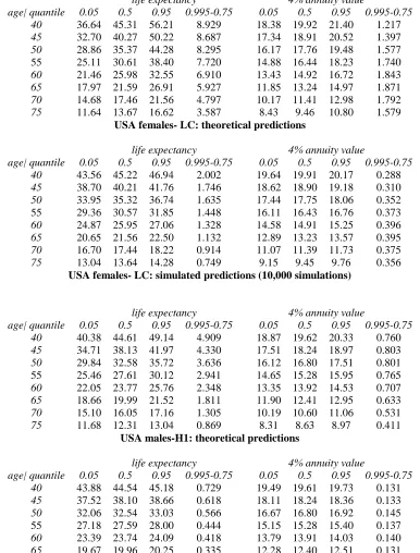
Using these parameters estimates and forecasts we tabulate (Table 1: 1st and 3rd panels) details for life expectancy and 4% annuity predictions, computed by cohort trajectory for ages 40, 45, 50, …75 focused on the year 2009. For convenience, we have not used the topping-out procedure advocated by Haberman and Renshaw (2012) for dealing with extrapolating the life table to the oldest ages. For comparison, we also tabulate (Table 1: 2nd and 4th panels) the respective equivalent life expectancies and 4% annuity predictions generated by the simulation method described in Haberman and Renshaw (2012), using a total of 10,000 simulations for each age. Referring to Table 1 and Figure 1 we note the following points:

 On comparing like for like, there is an exceptionally close agreement between the matching theoretical and simulated median predictions. However, the interval prediction widths in the theoretical cases are much wider when compared with the matching simulated cases.

 We note the narrowness of the simulated males prediction intervals, which are appreciably narrower than equivalent simulated intervals for the England & Wales male mortality experience depicted in Figure 8 of Haberman & Renshaw (2012), where topping-out by age has been applied but this seems to have little effect on increasing the interval widths.

 With the exception of a few isolated ages in the male experience, the beta parameters are positive over the full age range for males and females and therefore for both modelling structures. It would be possible to adapt the algorithms so that the beta parameters are constrained to be positive. We note further that the period index forecasts for mortality improvement rates are negative for males using H1 but positive for females using LC.

 In order to reach the 99.5% solvency probability required under Solvency 2, we assume that the policyholders are required to provide premiums adding up to the 75th quantile of the present value of annuity payments and the insurer pays for the difference between the 99.5th quantile of these payments and the aforementioned 75th quantile. Here, we make the assumption that the size of the portfolio is large enough to neglect diversifiable risk so that only the systematic risk matters. The latter is equal to the size of the portfolio multiplied by the expected present value of the annuity payments given future mortality. The difference in the 99.5th and 75th quantiles appears in the last column of each panel in Table 1. Comparing the differences based on the approximations derived in the present paper to the simulated ones, we see there that the amount of capital is over-estimated when the approximations are used.

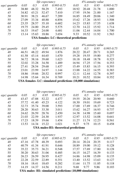
consistently higher than their matching counter-parts in Table 1 as expected. The approximations to the 95th quantiles listed in Table 1 are reasonably close to their simulated counterparts in Table 2 based on a reduction of death rates by 25%. This shows that the approximations derived in the present paper for high quantiles may be used as an alternative to the standard approach which involves decreasing all death rates by, say, 25%.

5. Discussion

Combining a conservative shift with non necessary conservative ones, the approximations derived in the present paper appear to be very accurate in the centre of the distribution (around the median) but tend to over estimate the tails (left and right). Using the proposed easy-to-compute approximation may thus be a good strategy for the calculation of the percentiles in the centre of the distribution (for example, the valuation of the median) as it would considerably reduce the computational burden and save time.

Acknowledgements

The authors would like to express their gratitude to an anonymous Referee whose comments have been extremely useful to revise a previous version of the present work. The financial support of PARC “Stochastic Modelling of Dependence” 2012-17 awarded by the Communauté française de Belgique is gratefully acknowledged by Michel Denuit.

References

Brouhns, N., Denuit, M., Vermunt, J.K. 2002. A Poisson log-bilinear approach to the construction of projected life tables. Insurance: Mathematics and Economics 31, 373-393.

Denuit, M. 2007. Distribution of the random future life expectancies in log-bilinear mortality projection models. Lifetime Data Analysis, 13, 381-397.

Denuit, M., Dhaene, J. 2007. Comonotonic bounds on the survival probabilities in the Lee-Carter model for mortality projection. Computational and Applied Mathematics 203, 169-176.

Denuit, M., Dhaene, J., Goovaerts, M.J., Kaas, R. 2005. Actuarial Theory for Dependent Risks: Measures, Orders and Models. Wiley, New York.

Denuit, M., Haberman, S., Renshaw A.E. 2010. Comonotonic approximations to quantiles of life annuity conditional expected present values: extensions to general ARIMA models and comparison with the bootstrap. ASTIN Bulletin 40, 331-349.

Haberman, S., Renshaw A.E. 2009. On age-period-cohort parametric mortality rate projections. Insurance: Mathematics and Economics 45, 255-270.

Haberman, S., Renshaw A.E. 2012. Parametric mortality improvement rate modelling and projecting. Insurance: Mathematics and Economics 50, 309-333.

Renshaw, A.E., Haberman, S. 2003. Lee-Carter mortality forecasting with age-specific enhancement. Insurance: Mathematics and Economics 33, 255-272.

life expectancy 4% annuity value

age| quantile 0.05 0.5 0.95 0.995-0.75 0.05 0.5 0.95 0.995-0.75

40 36.64 45.31 56.21 8.929 18.38 19.92 21.40 1.217

45 32.70 40.27 50.22 8.687 17.34 18.91 20.52 1.397

50 28.86 35.37 44.28 8.295 16.17 17.76 19.48 1.577

55 25.11 30.61 38.40 7.720 14.88 16.44 18.23 1.740

60 21.46 25.98 32.55 6.910 13.43 14.92 16.72 1.843

65 17.97 21.59 26.91 5.927 11.85 13.24 14.97 1.871

70 14.68 17.46 21.56 4.797 10.17 11.41 12.98 1.792

75 11.64 13.67 16.62 3.587 8.43 9.46 10.80 1.579

USA females- LC: theoretical predictions

life expectancy 4% annuity value

age| quantile 0.05 0.5 0.95 0.995-0.75 0.05 0.5 0.95 0.995-0.75

40 43.56 45.22 46.94 2.002 19.64 19.91 20.17 0.288

45 38.70 40.21 41.76 1.746 18.62 18.90 19.18 0.310

50 33.95 35.32 36.74 1.635 17.44 17.75 18.06 0.352

55 29.36 30.57 31.85 1.448 16.11 16.43 16.76 0.373

60 24.87 25.95 27.06 1.328 14.58 14.91 15.25 0.396

65 20.65 21.56 22.50 1.132 12.89 13.23 13.57 0.395

70 16.70 17.44 18.22 0.914 11.07 11.39 11.73 0.375

75 13.04 13.64 14.28 0.749 9.15 9.45 9.76 0.356

USA females- LC: simulated predictions (10,000 simulations)

life expectancy 4% annuity value

age| quantile 0.05 0.5 0.95 0.995-0.75 0.05 0.5 0.95 0.995-0.75

40 40.38 44.61 49.14 4.909 18.87 19.62 20.33 0.760

45 34.71 38.13 41.97 4.330 17.51 18.24 18.97 0.803

50 29.84 32.58 35.72 3.636 16.12 16.80 17.51 0.801

55 25.46 27.61 30.12 2.941 14.65 15.28 15.95 0.765

60 22.05 23.77 25.76 2.348 13.35 13.92 14.53 0.707

65 18.66 19.99 21.52 1.811 11.90 12.41 12.95 0.633

70 15.10 16.05 17.16 1.305 10.19 10.60 11.06 0.531

75 11.68 12.31 13.04 0.869 8.31 8.63 8.97 0.411

USA males-H1: theoretical predictions

life expectancy 4% annuity value

age| quantile 0.05 0.5 0.95 0.995-0.75 0.05 0.5 0.95 0.995-0.75

40 43.88 44.54 45.18 0.729 19.49 19.61 19.73 0.131

45 37.52 38.10 38.66 0.618 18.11 18.24 18.36 0.133

50 32.06 32.54 33.03 0.566 16.67 16.80 16.92 0.145

55 27.18 27.59 28.00 0.444 15.15 15.28 15.40 0.137

60 23.39 23.74 24.09 0.418 13.79 13.91 14.03 0.140

65 19.67 19.96 20.25 0.335 12.28 12.40 12.51 0.131

70 15.81 16.03 16.25 0.267 10.49 10.59 10.69 0.122

75 12.13 12.29 12.46 0.193 8.53 8.62 8.70 0.100

[image:12.612.113.499.92.600.2]

USA males- H1: simulated predictions (10,000 simulations)

life expectancy 4% annuity value

age| quantile 0.05 0.5 0.95 0.995-0.75 0.05 0.5 0.95 0.995-0.75

40 38.80 48.32 58.29 7.493 18.92 20.48 21.78 1.000

45 34.82 43.21 52.47 7.410 17.95 19.56 21.00 1.167

50 30.91 38.21 46.67 7.209 16.85 18.49 20.06 1.340

55 27.09 33.34 40.88 6.856 15.62 17.26 18.93 1.508

60 23.35 28.57 35.10 6.602 14.23 15.83 17.55 1.638

65 19.75 24.00 29.45 5.575 12.70 14.22 15.92 1.714

70 16.33 19.67 24.00 4.681 11.06 12.44 14.04 1.700

75 13.14 15.63 18.86 3.654 9.33 10.52 11.92 1.563

USA females- LC: theoretical predictions

life expectancy 4% annuity value

age| quantile 0.05 0.5 0.95 0.995-0.75 0.05 0.5 0.95 0.995-0.75

40 46.51 48.22 49.94 1.876 20.22 20.47 20.71 0.265

45 41.58 43.14 44.65 1.670 19.28 19.55 19.80 0.277

50 36.72 38.16 39.60 1.623 18.18 18.48 18.78 0.323

55 32.02 33.28 34.58 1.489 16.94 17.25 17.56 0.353

60 27.41 28.54 29.68 1.437 15.49 15.83 16.15 0.393

65 23.01 23.99 24.97 1.144 13.88 14.22 14.55 0.383

70 18.86 19.66 20.52 0.997 12.11 12.44 12.78 0.397

75 14.98 15.64 16.34 0.769 10.21 10.52 10.84 0.352

USA females- LC: simulated predictions (10,000 simulations)

life expectancy 4% annuity value

age| quantile 0.05 0.5 0.95 0.995-0.75 0.05 0.5 0.95 0.995-0.75

40 43.47 47.88 52.22 4.477 19.55 20.26 20.90 0.660

45 37.72 41.40 45.23 4.122 18.30 19.01 19.69 0.723

50 32.73 35.74 39.00 3.593 17.00 17.69 18.37 0.746

55 28.20 30.63 33.30 3.011 15.62 16.27 16.93 0.737

60 24.62 26.59 28.76 2.450 14.38 14.98 15.60 0.697

65 21.03 22.59 24.30 1.937 12.97 13.52 14.08 0.641

70 17.23 18.39 19.66 1.454 11.27 11.74 12.23 0.561

75 13.53 14.34 15.22 1.021 9.37 9.75 10.15 0.458

USA males-H1: theoretical predictions

life expectancy 4% annuity value

age| quantile 0.05 0.5 0.95 0.995-0.75 0.05 0.5 0.95 0.995-0.75

40 47.16 47.78 48.39 0.693 20.14 20.24 20.35 0.117

45 40.79 41.34 41.91 0.646 18.89 19.00 19.12 0.128

50 35.22 35.73 36.21 0.548 17.57 17.69 17.80 0.128

55 30.20 30.63 31.06 0.485 16.15 16.27 16.39 0.133

60 26.23 26.59 26.95 0.427 14.86 14.98 15.09 0.135

65 22.28 22.59 22.89 0.351 13.40 13.52 13.63 0.127

70 18.16 18.41 18.65 0.282 11.64 11.75 11.85 0.118

75 14.19 14.37 14.56 0.211 9.68 9.77 9.86 0.103

[image:13.612.117.494.86.643.2]

USA males- H1: simulated predictions (10,000 simulations)

Table 2. USA female & male 2009 life expectancy and 4% annuity quantile predictions, ages 40(05)75: comparison of theoretical & simulated predictions subject to a 25%