Design and tuning of fractional-order PID controllers for time-delayed processes

(1)

Design and Tuning of Fractional-order PID

Controllers for Time-delayed Processes

Emmanuel Edet

Technology and Innovation Centre

University of Strathclyde 99 George Street Glasgow, United Kingdom [email protected]

Reza Katebi

Industrial Control Centre University of Strathclyde Glasgow, United Kingdom

[email protected]

Abstract— Frequency domain based design methods are investigated for the design and tuning of fractional-order PID for scalar applications. Since Ziegler-Nichol’s tuning rule and other algorithms cannot be applied directly to tuning of fractional-order controllers, a new algorithm is developed to handle the tuning of these fractional-order PID controllers based on a single frequency point just like Ziegler-Nichol’s rule for inter order PID. Critical parameters of the system are obtained at the ultimate point and the controller parameters are calculated from these critical measurements to meet design specifications. Thereafter, fractional order is obtained to meet a specified robustness criteria which is the phase-invariability against gain variations around the phase cross-over frequency. Results are simulated on second –order plus dead time plant to demonstrate both performance and robustness.

Keywords—robustness; performance; tuning; PID

I. INTRODUCTION

In recent years, interesting control engineering applications have been developed using differential equations of generalized order ‘𝛼′where the derivative order 𝛼 can be any non-integer. Control systems utilizing fractional dynamics termed fractional order control systems have been found to yield better performance than integer-order controllers under fair comparison [1].

A. Some Definitions of Fractional-order Derivative

Consider the generalised-order differential equation (1)

shown below:

𝑦(𝑡) = 𝒟α _{𝑢(𝑡) + 𝑢(𝑡) (1)} 𝑤ℎ𝑒𝑟𝑒 𝑡 > 0; 𝑛 − 1 < 𝛼 < 𝑛; 𝑛 ∈ ℝ

Equation 1 is a fractional order differential equation as far as the order "α" is non-integer. There are two important definitions that allow for computation of fractional order derivative namely:

 Caputo’s Fractional order derivative  Riemann-Liouville Definition.

Fractional –order derivative with order (𝛼) is defined by Riemann-Liouville as:

𝒟α _{𝑓(𝑡) ≜ 𝒟}n _ℓn−α _𝑓(𝑡)

= 𝑑

𝑛

𝑑𝑡𝑛[

1

Γ(𝑛 − 𝛼)∫

𝑓(𝜏)

(𝑡 − 𝜏)𝛼−𝑛+1

𝑡

0

] 𝑑𝜏. (2)

𝑤ℎ𝑒𝑟𝑒 𝑡 > 0; 𝑛 − 1 < 𝛼 < 𝑛; 𝑛 ∈ ℝ.

An alternative definition was also given by Caputo [2] as shown in equation 3:

𝒟𝛼_{𝑓(𝑡) ≜ ℓ}n−α _𝒟n _𝑓(𝑡)

= [ 1

Γ(𝑛 − 𝛼)∫

𝑓𝑛(𝜏)

(𝑡 − 𝜏)𝛼−𝑛+1

𝑡

0

𝑑𝜏] (3)

𝑡 > 0; 𝑛 − 1 < 𝛼 < 𝑛; 𝑛 ∈ ℝ

However, the inclusion of the nth order derivative of f(t) in Caputo’s definition imposes restriction compared to Riemann-Liouville form [3].

B. Fractional-order PID

The theory of fractional dynamics has been utilized to design PIDs with non-integer order - PID. Fractional order PID Controllers (PID) have been extensively tested in demanding applications especially in mechatronic and automatic control applications and are found to yield very good results [2]. Basically, PID is of the form:

𝐶(𝑠) = 𝐾𝑝+

𝐾𝑖

s𝜆+ 𝐾𝑑𝑠

𝜇₍₄₎

where:

 and  are the fractional orders of integral and derivative parts of the controller respectively. Therefore there are five parameters that are to be determined: KP, KI, KD, , and . It

(2)

II. SPECIFICATION OF DESIGN OBJECTIVES

The first step is to define design specifications expected to be satisfied by the fractional order controller. These design objectives are defined in frequency domain in order to take care of important control objectives: stability, performance and robustness. Each controller parameter can be tuned to satisfy each design specification.

A. Gain Margin and Phase Cross-over Frequency Specification.

Gain margin is a primary index of relative stability in classical control design. A pre-defined margin can be used to formulate a robustness constraint on the system gain. Equation I defines the relationship between gain margin and phase cross over frequency while equation 5 defines the gain margin constraint:

|𝐶(𝑗𝜔𝑐𝑔)𝐺(𝑗𝑤𝑐𝑔)| 𝑑𝐵 = 0 𝑑𝐵 (5)

|𝐶(𝑗𝜔𝑐𝑝)𝐺(𝑗𝑤𝑐𝑝)| 𝑑𝐵 =

1

𝐴𝑚

(6)

where:

𝜔

𝑐𝑔

-

The gain crossover frequency

𝑤

𝑐𝑝

–

Phase cross over frequency

𝐴𝑚 – The Gain margin.

B.Phase Margin and Gain Crossover Frequency Specification

Phase margin and gain margin are extended to fractional order control as useful measures of robust stability. It is chosen to satisfy equation 7

arg (𝐶(𝑗𝜔𝑐𝑔)𝐺(𝑗𝑤𝑐𝑔)) = −𝜋 + ∅𝑚 (7)

C.Robustness against Plant’s Gain Variations

Bode’s ideal loop defines the criteria for absolutely stable SISO loop. As long as the open loop gain is defined by a constant phase around the crossover frequency (useful band), robust stability against gain variations is guaranteed within that frequency range of constant phase.

𝑑{arg(𝐶(𝑗𝜔)𝐺(𝑗𝜔))}

𝑑𝜔 = 0 𝑎𝑟𝑜𝑢𝑛𝑑 𝜔𝑐𝑔. (8)

The phase of the forward loop function will be flat around the cross over frequency. This improves robustness against gain-like variations in plant and the overshoot is nearly constant within that given frequency range.

D.High frequency noise rejection specification

In order to ensure satisfactory measurement noise rejection, appropriate bound for the complementary sensitivity function has to be defined:

‖𝑇(𝑗𝜔)‖_𝑑𝐵≤ 𝐴 𝑑𝐵

‖ 𝐶(𝑗𝜔)𝐺(𝑗𝜔)

1+𝐶(𝑗𝜔)𝐺(𝑗𝜔)‖_𝑑𝐵≤ 𝐴 𝑑𝐵 for ω ≥ 𝜔𝑡 rad/s. (9)

where

:

T(𝑗𝜔)is the complementary sensitivity function

.

A dB = the specified attenuation level in dB for the band 𝜔 ≥

𝜔𝑡

𝑟𝑎𝑑

𝑠 .

E.Output disturbance rejection specification.

Sensitivity bound can be defined to ensure satisfactory output disturbance rejection by the controller:

‖ 1

1+𝐶(𝑗𝜔)𝐺(𝑗𝜔)‖_𝑑𝐵≤ 𝐵 𝑑𝐵 (10)

where

:

B dB = the specified magnitude of the sensitivity function in

dB for the band

𝜔 ≤ 𝜔

_𝑠𝑟𝑎𝑑

𝑠

.

In addition, the nth-fractional integral term ensures steady state error rejection as effectively as an equivalent integer-order integral controller due to the implementation as 𝑠−1_𝑠1−𝑛_{. Five} parameters are available for tuning in order to meet five specifications. The proportional gain, integral gain, derivative gain, derivative (fractional) order and the fractional order of the integral term are available parameters that can be optimised to meet the defined specifications [3]. This is the primary reason behind the superior control action of fractional order controller type over the integer order types – more parameters are available for optimization to meet more control objectives. Monje [3, 5] used MATLAB’s optimization tool (fmincon) to formulate an optimization problem that solves for these five parameters and it was a constraint non-linear optimization problem with five unknown variables. Another way of obtaining robust values for PID controller gains is to use sustained oscillation method as described next while the fractional order for the integral controller term can be chosen to satisfy robust performance criteria. This method reduces computational cost.

III. THE ULTIMATE POINT PARAMETER METHOD

In industrial circles, Ziegler-Nichols PID tuning rule and similar PID design methods are still dominant for simple process models. In this section, a similar technique is developed for SISO processes. The basic principle involves using a proportional controller in cascade with the plant under a closed loop configuration. Thereafter, the proportional gain is systematically increased from very small values until sustained oscillation or continuous cycling is observed at the process output. The value of the proportional gain that yields this sustained oscillation is recorded as the critical gain (𝐾𝑢) while the period of oscillation is noted as the ultimate period 𝑇𝑢.

Several other important information about the process are obtainable from these critical point measurements. For instance, the phase cross over frequency can be obtained as:

𝜔𝑝𝑐𝑜=

2𝜋 𝑇𝑢

(11)

(3)

[image:3.612.85.313.65.263.2]

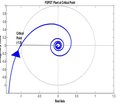
Fig. 1. Nyquist Diagram indicating Plant’s Critical Point

A. Design of the Fractional-order PI controller

Consider a fractional PI controller of the form:

𝐶(𝑠) = 𝐾𝑝+

𝐾𝑖

𝑠𝛼 (12)

𝐶(𝑗𝜔) = 𝐾𝑝+ 𝐾𝑖

(𝑗𝜔)𝛼

𝐾𝑖=

𝐾𝑝

𝑇𝑖

A desirable point on the complex plane is chosen as design point - B given as (𝑟𝐵𝑒𝑗(𝜋+∅𝐵)_).

The controller is expected to move the ultimate point (1 𝐾𝑢 , 0 )

to this desirable point. On the Nyquist plot, the ultimate point is - point A (𝑟𝐴𝑒𝑗𝜋)).

𝑟𝐴 = 1

𝐾_𝑢 (13)

Finally, Let the frequency characteristic of the controller C(s) be 𝑟𝐶𝑒𝑗(𝜋+∅𝐶). For this controller to move the ultimate point to the desirable point on the complex plane, equation 14

must be satisfied:

⇒ 𝑟𝐴𝑟𝐶𝑒𝑗𝜋_𝑒𝑗(𝜋+∅𝐶)_{= 𝑟𝐵𝑒}𝑗(𝜋+∅𝐵)₍₁₄₎_.

𝑟𝐶𝑒𝑗(𝜋+∅𝐶)₌𝑟𝐵

𝑟𝐴(cos ∅𝐵+ 𝑗 sin ∅𝐵) (15)

𝑟𝐶𝑒𝑗(𝜋+∅𝐶)= 𝑟𝐵𝐾𝑢(cos ∅𝐵+ 𝑗 sin ∅𝐵)

Therefore, the fractional-order PI controller is chosen to satisfy the magnitude and phase conditions below in 16 and 17:

𝑟𝐶 =

𝑟𝐵 𝑟𝐴

(16)

∅𝐶 = ∅𝐵− 0 (17)

Recall the controller structure in frequency domain as given in equation 12:

𝐶(𝑗𝜔) = 𝐾𝑝+

𝐾𝑖

(𝑗𝜔)𝛼

𝐶(𝑗𝜔) = 𝐾( 1 + 1

(𝜏𝑖)(𝑗𝜔)𝛼)

𝐶(𝑗𝜔) = 𝐾(1 + 1

𝜔𝛼_𝜏 𝑖(cos

𝛼𝜋

2 − 𝑗 sin

𝛼𝜋

2 ) ) (18)

⇒ 𝐾(1 + 1

𝜔𝛼_𝜏𝑖(cos

𝛼𝜋

2 − 𝑗 sin

𝛼𝜋

2 ) )

= 𝑟𝐵𝐾𝑢(cos ∅𝐵+ 𝑗 sin ∅𝐵).

Comparing magnitudes:

𝑟𝐵𝐾𝑢cos ∅𝐵 = 𝐾 (1 +

1

𝜔𝛼_𝜏

𝑖

(cos𝛼𝜋

2 )) (19)

In the same vein, arguments are compared and the phase is expected to fulfil equation 20 below:

tan ∅𝐵 = −𝜔

−𝛼_𝜏

𝑖−1sin 𝛼𝜋/2

(1 + 𝜔−𝛼_𝜏

𝑖−1cos 𝛼𝜋/2)

(20)

If we set 𝑦 = 1 𝜏𝑖;

𝑦 = − tan ∅𝐵

𝜔−𝛼_{(tan ∅}

𝐵cos

𝛼𝜋

2 + sin 𝛼𝜋/2)

(21)

B. Justification of Design Point

The desired point B is chosen such that 𝑟𝐵=

0.29 𝑎𝑛𝑑 ∅𝐵= 46 𝑑𝑒𝑔.

This is a very desirable point because it translates to -0.2-j0.21 point. The distance from this point to the stability limit (-1,j0)

is 𝑑 = √(−0.2 + 1)2_{+ (−0.21)}2_{which is approximately 0.9.}

Closed loop sensitivity can be deduced from this information on the Nyquist curve of the forward loop because the maximum sensitivity 𝑀𝑠 is the reciprocal of the shortest distance from the Nyquist curve to the critical point.

By definition: 𝑀𝑠= max

0≤𝜔≤∞|

1

1+𝐶(𝑠)𝐺(𝑠)|. However, on the Nyquist curve, 𝑀𝑠=

1 𝑑.

⇒ 𝑀𝑠=

1

0.9= 1.1

This is very desirable for robustness. For the closed loop system to be robust against variations in process dynamics, maximum sensitivity of the closed loop system is specified:

𝑀𝑠 < 2. Reasonable values of 𝑀𝑠ranges from 1.05 to 1.95.

This indicates good robustness for many practical control applications and it is therefore recommended as the design point as far as single frequency point method is concerned throughout this paper. This design point is also justified as far as closed loop stability is concerned. It meets Nyquist stability criterion as the critical stability (-1,0) point will not be encircled. Therefore, the fractional order PI controller can be obtained from 22 and 23.

𝐾 = 0.202𝐾𝑢− (

𝜏𝑢

2𝜋)

𝛼_cos𝛼𝜋

2 (22)

-1 -0.5 0 0.5 1 1.5

-1 -0.8 -0.6 -0.4 -0.2 0 0.2 0.4 0.6 0.8

1 FOPDT Plant at Critical Point

Real Axis

I

m

a

g

i

n

a

r

y

A

x

i

s

(4)

[image:4.612.317.541.377.527.2]

|𝜏𝑖| = 0.966 (𝜏𝑢

2𝜋)

𝛼_(sin𝛼𝜋

2 + 1.036𝑐𝑜𝑠

𝛼𝜋

2) (23)

Fractional order is selected to meet the required resonant peak 𝑀𝑟condition as given by Monje for SISO-FOPDT systems. This is sufficient for SISO control problems with FOPDT process model.

𝐺(𝑠) =𝑌𝑒−𝐿𝑠

𝑠𝜏+1. Relative dead-time is: 𝑇 = 𝐿

𝐿+𝜏 (24).

TABLE I. RELATIVE DEAD TIME AND FRACTIONAL-ORDER

For Second order processes such as SOPDT (Second Order Plus Dead-Time model), derivative component can be included for a more damped response. One possible solution is to design the fractional controller in the form of 𝑃𝐼𝜇_𝐷_{-structure. It is} however tuned in a similar fashion as the fractional PI case using ultimate parameters.

C. The 𝑃𝐼𝜇_𝐷_{- Structure}

The structure of the controller is given as:

𝐾𝑖

(𝑗𝜔)𝛼+ 𝐾𝐷(𝑗𝜔) (25)

𝐶(𝑗𝜔) = 𝐾𝑝(1 +

1

𝜏𝑖(cos𝛼𝜋₂ + 𝑗 sin𝛼𝜋₂) 𝜔𝛼

+ 𝜏𝐷(𝑗𝜔) (26)

Let the controller 𝐶(𝑗𝜔) be characterised by 𝑟𝐶𝑒𝑗(𝜋+∅𝐶) in frequency domain and the desirable point on the Nyquist plane chosen as point B that is: (𝑟𝐵𝑒𝑗(𝜋+∅𝐵)₎_{as earlier given.}

The controller is expected to move the ultimate point (1 𝐾𝑢 , 0 )

to this desirable point as earlier explained in previous section. On the complex plane, the ultimate point is - point A (𝑟𝐴𝑒𝑗𝜋)_). Therefore, equations 14, 15 and 16 must be fulfilled as earlier shown. It follows that:

(𝐾𝑝(1 +

1

𝜏𝑖(cos 𝛼𝜋

2 + 𝑗 sin

𝛼𝜋

2) 𝜔𝛼

+ 𝜏𝐷(𝑗𝜔) )

=𝑟𝐵

𝑟𝐴

cos(∅𝐵− ∅𝐴) (27)

Consider the argument:

tan(∅𝐵− ∅𝐴) =

𝜔𝜏𝐷−

1

𝜔𝛼_𝜏𝑖sin( 𝛼𝜋/2)

1 +_𝜔1𝛼_𝜏

𝑖cos(𝛼𝜋/2)

Given that the ultimate point is to be moved; ∅𝐴= 0.

tan ∅𝐵(1 +

1

𝜔𝛼_𝜏

𝑖

cos (𝛼𝜋

2 )) = 𝜔𝜏𝐷−

1

𝜔𝛼_𝜏

𝑖

sin ( 𝛼𝜋/2)

Making 𝜏𝑖 subject of formular and substituting 𝜔 =2𝜋 𝑇𝑢

yields:

𝜏𝑖 =

𝜏𝑢𝛼_{(𝑡𝑎𝑛∅𝐵}_cos𝛼𝜋

2 + sin

𝛼𝜋

2)

(2𝜋)𝛼₍2𝜋𝜏𝐷

𝜏𝑢 − 𝑡𝑎𝑛∅𝐵)

(28)

𝐾𝑝= 𝑟𝐵𝐾𝑢cos ∅𝐵−

𝜏𝑢𝛼cos 𝛼𝜋

2

((2𝜋)𝛼_𝜏

𝑖)

(29)

Given that the order α is obtainable as before from the 𝑀𝑟table, there are now three parameters left to be obtained from two equations. This is clearly insufficient. One way to solve it is to treat the ratio of 𝜏𝐷 𝑡𝑜 𝜏𝑖 as a constant [6]. For instance:

𝜏𝐷 = 0.25𝜏𝑖.

All four parameters can therefore be calculated.

The second structure of fractional controller with derivative component is of PIDα form.

D. The PIDα Controller form.

𝐾𝑖

𝑗𝜔+ 𝐾𝐷(𝑗𝜔)

𝛼₍₃₀₎

𝐶(𝑗𝜔) = 𝐾𝑝(1 − 𝑗

1 𝜏𝑖𝜔

+ 𝜏𝐷(𝑗𝜔)𝛼 )

The controller structure is given in equation 30. It is expected to move the ultimate point to our new design point B implying that equations 14, 15 and 16 applies again as stated in previous sections. Therefore:

(𝐾𝑝(1 + 𝜔𝛼𝜏𝐷cos(𝛼𝜋/2)) =

𝑟𝐵 𝑟𝐴

cos(∅𝐵− ∅𝐴)

𝐾𝑝=

𝑟𝐵

𝑟𝐴cos(∅𝐵− ∅𝐴)

1 + 𝜔𝛼_𝜏𝐷_cos𝛼𝜋

2

𝐾𝑝= 𝑟𝐵𝐾𝑢cos(∅𝐵)

1 + 𝜔𝛼_𝜏

𝐷cos

𝛼𝜋 2

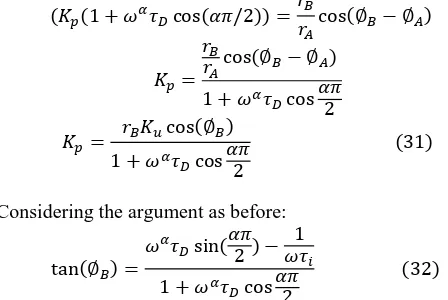
(31)

Considering the argument as before:

tan(∅𝐵) =

𝜔𝛼_𝜏

𝐷sin(𝛼𝜋₂) −_𝜔𝜏1

𝑖

1 + 𝜔𝛼_𝜏𝐷_cos𝛼𝜋

2

(32)

The ratio of integral time to derivative time is set to constant as before: 𝜏𝐷 = 0.25𝜏𝑖 and equations 32 and 31 gives the two controller parameters. Fractional order are obtained in similar fashion to previous cases using the peak resonant condition.

IV. RESULTS OF SISOPLANT SIMULATIONS

Consider a FOPDT plant given as

𝐺(𝑠) = 12.8𝑒

−𝑠

16.7𝑠 + 1

Three controllers C1, C2 and C3 are designed in the following

forms: 𝑃𝐼𝜇_{, PI}μ_D_and_PIDα_{respectively. This is done using the} sustained oscillation method as described in this work:

Cases ∝ - order Relative Dead-time T

1. 0.7 𝑇 < 0.1

2. 0.9 0.1 ≤ 𝑇 < 0.4

3. 1.0 0.4 ≤ 𝑇 < 0.6

(5)

Fig. 2. Nyquist Diagram of FOPDT Plant with controller C1

𝐶1= 0.04(1 +

1

1.12𝑠0.7)

𝑠−0.7_{is implemented as}_𝑠0.3_𝑠−1_{using the well-known ORA} approximation (Oustaloup Recursive Approximation) inorder to obtain integer order form of the controller with the same frequency domain properties [7, 8]. ORA has been reported by many authors as a good approximation to the fractional order. Therefore, it is used throughout this work to realise a rational and implementable function.

𝐶2= 0.32(1 +

0.1

𝑠0.7+ 0.35𝑠)

𝐶3= 0.218(1 +

1

3.6𝑠+ 1.08𝑠

0.7₎

It is observed that the controller moves the design point of the plant in figure 1 to a desired (stable) region as shown in Nyquist diagrams shown next:

Consider a second example - a SOPDT plant below:

𝐺

2

(𝑠) =

2𝑒

−0.2𝑠

𝑠(0.5𝑠 + 1)

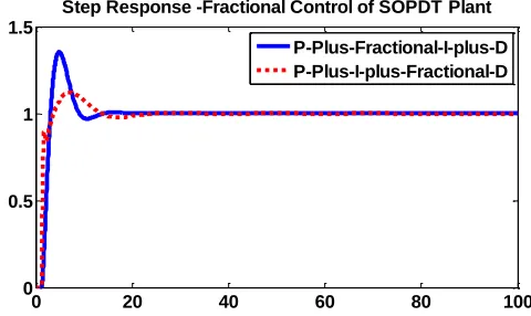
The controller realized using 𝑃𝐼𝜇_𝐷_{structure as earlier} discussed is: 𝐶22(𝑠) = 0.459 +

0.2

𝑠0.9+ 0.28𝑠.

The fractional controller of the form PIDα is also realized as C11 given below: 𝐶11= 0.444 +

0.175

𝑠 + 0.3𝑠

0.9_.

Performance is compared using Bode diagram of figure 5and step response shown in figure 6.

Fig. 5. Bode Diagram of SOPDT Plant with controller C11 and C22 -50

0 50 100 150

M

a

g

n

it

u

d

e

(

d

B

)

10-4 10-3 10-2 10-1 100 101 102

-1080 -720 -360 0

P

h

a

s

e

(

d

e

g

)

Control of SOPDT plant

Frequency (rad/s)

c22 c11

C11 GAIN MARGIN: 1.1

C11 PHASE MARGIN: 7.13

C11 DELAY MARGIN: 0.02

C22 GAIN MARGIN: 7.4

C22 PHASE MARGIN: 53.4

C22 DELAY MARGIN: 1.02 -1 -0.8 -0.6 -0.4 -0.2 0 0.2 0.4 0.6 0.8 1

-1 -0.8 -0.6 -0.4 -0.2 0 0.2 0.4 0.6 0.8

1 FOPDT with C1

Real Axis

Im

a

g

ina

ry

A

x

is Gain Margin: 13.2 dB

Phase Margin: 44.7 deg Delay Margin: 4.5

-1 -0.8 -0.6 -0.4 -0.2 0 0.2 0.4 0.6 0.8 1

-1 -0.8 -0.6 -0.4 -0.2 0 0.2

FOPDT with C2

Real Axis

Im

a

g

in

a

ry

A

x

is

Gain Margin: 7.1 dB Phase Margin: 69.7 deg Delay Margin: 4.05

-1 -0.8 -0.6 -0.4 -0.2 0 0.2

-1 -0.8 -0.6 -0.4 -0.2 0

0.2 FOPDT with C3

Real Axis

Im

a

g

in

a

ry

A

x

is

Gain Margin: 3.3 dB

Phase Margin: 76.7 deg

(6)

V. DISCUSSION OF RESULTS AND CONCLUSION

These SISO based methods yield excellent response for the plants examined as reflected in the gain margin, phase margin and delay margin. The delay margin is an important robustness measure which gives information about how much time delay can be introduced to the system before it goes unstable. In addition, very little computation is required to yield the desired fractional controller.In summary, the main contribution of this paper is development of a new design method for fractional-order PID (FPID) controller. Extended simulations has been carried out on delayed processes with FOPDT and SOPDT dynamics. It has been found to yield control actions with good compromise between robustness and performance.

VI. REFERENCES

[1] Z. Li and Y. Chen, "Ideal, Simplified and Inverted Decoupling of Fractional order TITO Processes," in

IFAC, Cape Town, 2014.

[2] I. Podlubny, "Fractional-Order Sysmtems and PID Controllers," IEEE Transactions on Automatic Control,

vol. 44, no. 1, pp. 208-214, 1999.

[3] C. Monje, Y. Chen, B. D. Vinagre and V. Feliu, Fractional-order Systems and Controls: Fundamentals and Applications, London: Springer-Verlag, 2010. [4] G. Vinagre, D. Valerio and J. Costa, "Rule-Tuned PIDs

and Fractional PIDs for a Three-Tank Liquid System," in

Symposium on Fractional Signals and Systems, Lisbon, Portugal, 2009.

[5] C. Monje, Y. Chen, D. Vinagre and V. Feliu, "Tuning and Auto-tuning of Fractional order Controllers for Industry Applications," Control Engineering Practice,

vol. 16, pp. 798-812, 2008.

[6] K. Astrom and T. Hagglund, Advanced PID Control, Durham, USA.: ISA, 2006.

[7] D. Valerio and S. Costa, "Time domain implementation of Fractional order controllers," IEEE Transaction on Control Theory Application, vol. 152, no. 5, pp. 539-552, 2005.

[8] F. Merrikh-Bayat, "Rules for Selecting the Parameters of Oustaloup Recurssive Approximation for the Simulation of Linear Feedback Systems containing Fractional PID controller," Nonlinear Science and Numerical Simulation,

[image:6.612.335.575.56.199.2]

vol. 17, pp. 1852-1861, 2012.

Fig. 6. Diagram of step response SOPDT Plant with controller C11 and C22

0 20 40 60 80 100

0 0.5 1 1.5

Step Response -Fractional Control of SOPDT Plant