Forecasting exchange rate volatility: GARCH models versus implied volatility forecasts

City, University of London Institutional Repository

Citation

: Pilbeam, K. and Langeland, K. N. (2014). Forecasting exchange rate volatility:

This is the unspecified version of the paper.

This version of the publication may differ from the final published

version.

Permanent repository link:

Link to published version

: http://dx.doi.org/10.1007/s10368-014-0289-4

Copyright and reuse:

City Research Online aims to make research

outputs of City, University of London available to a wider audience.

Copyright and Moral Rights remain with the author(s) and/or copyright

holders. URLs from City Research Online may be freely distributed and

linked to.

City Research Online: http://openaccess.city.ac.uk/ publications@city.ac.uk

1

Keith Pilbeam and Kjell Noralf Langeland

CITY UNIVERSITY LONDON

Forecasting Exchange Rate Volatility: GARCH models versus Implied Volatility Forecasts

Abstract

This study investigates whether different specifications of univariate GARCH models can usefully forecast volatility in the foreign exchange market. The study compares in-sample forecasts from symmetric and asymmetric GARCH models with the implied volatility derived from currency options for four dollar parities. The data set covers the period 2002 to 2012. We divide the data into two periods one for the period 2002 to 2007 which is characterised by low volatility and the other for the period 2008 to 2012 characterised by high volatility. The results of this paper reveal that the implied volatility forecasts significantly outperforms the three GARCH models in both low and high volatility periods. The results strongly suggest that the foreign exchange market efficiently prices in future volatility.

Please note this is the public version of the paper, the final paper appears in International Economics and Economic Policy. Corresponding author Keith Pilbeam

Keywords Exchange Rate, Volatility Modelling

Acknowledgements

2 1. Introduction

The foreign exchange market is by far the largest and most liquid financial market in

the world. As reported by the Bank for International Settlement in April 2013 the

average daily turnover was $5.0 trillion. The foreign exchange market is made up

primarily of three inter-related parts; spot transactions, forward transactions and

derivative contracts. As with other financial markets currency markets can be volatile

and exhibit periods of volatility clustering as traders react to new information.

Improving the forecasting of volatility in the foreign exchange market is important

to multinational firms, financial institutions and traders wishing to hedge currency

risks. Volatility is usually defined as the standard deviation or variance of the returns

of an asset during a given time period. Traders of foreign currency options attempt to

make profits by buying options if they expect volatility to rise above that implied in

currency option premiums and writing options if they expect volatility to be lower

than that currently implied by option premiums.

This paper examines the efficiency of the foreign exchange market in pricing

option volatility by comparing the forecasts given the implied volatility from currency

option prices with volatility forecasts from three different univariate GARCH models.

If the foreign exchange market is efficient, then the implied volatility forecasts should

outperform the GARCH forecasts. In addition, as Engle and Patton (2001) the whole

point of GARCH forecasting models is that they should help in forecasting future

volatility and as such see whether they can beat implied volatility forecasts is an

interesting topic in itself. Our period of study which covers the period 2002 – 2012 is

3

which also resulted in a noticeable increase in turbulence in the foreign exchange

market.

The paper is organized as follows section 2 gives a review on the three

univariate GARCH models we use for our empirical forecasting exercise. Section 3

gives a more detailed introduction to the models being used and the estimation of

volatility. Section 4 looks at the features of the data set and its properties. In section 5

we present the results of the study and section 6 concludes.

2. Review of the use of GARCH Models

In the last decade, forecasting exchange rate volatility has been a very popular topic in

economic journals, see for example Busch et al (2012). Using different time periods,

data frequency and the exchange rate pairs research has used a wide range of

volatility models. Conditional variance models, such as ARCH and GARCH are the

most often used to forecast volatility. In this study, we use both symmetric and

asymmetric GARCH models (1). The symmetric model we use is the GARCH (1,1)

of Bollerslev (1986) and Taylor (1986) the GARCH(1,1) model is far more widely

used than ARCH due to the fact that it is more parsimonious and avoids over fitting

(2) and is consequently less likely to breach the non-negativity constraint. We also

look at two asymmetric models the EGARCH of Nelson (1991) and GJR-GARCH of

Glosten, Jagannathan, and Runkle (1993). The EGARCH model has two key

advantages over the GARCH (1,1). Firstly, the model measures the log returns, and

therefore even if the parameters are negative, the conditional variance will be

positive. Secondly, the model allows for asymmetries can capture the so called

leverage effect (3). The second asymmetric model we use if the GJR-GARCH model

4

that is added to capture possible asymmetries. (4).We compare the forecasts of

these models to the implied volatility series provided on bloomberg.

Bollerslev (1986) showed that the GARCH model outperformed the ARCH

model. However, Baillie and Bollerslev (1991) used the GARCH model to

examine patterns of volatility in the US forex market and results were generally

poor. In the two decades after the arrival of ARCH and GARCH, several

approaches building on GARCH has been created. EGARCH was introduced by

Nelson (1991), NGARCH by Higgins and Bera (1992), GJR-GARCH by Glosten,

Jagannathan and Runkle (1993), TGARCH by Zakoian (1994), QGARCH by

Sentana (1995), and many more are available see for example Bollerslev (2008).

In an interesting study, Hansen and Lunde (2005) finds that none of the models

in the GARCH family outperforms the simple GARCH (1,1) which might be

surprising since the GARCH (1,1) does not rely upon a leverage effect. While

Nelson`s EGarch has several advantages over the linear GARCH model authors

such as Brownlees and Gallo (2010) find that while at some horizons EGARCH

produces the most accurate forecast, but at other horizons EGARCH is

outperformed by the linear GARCH model. Donaldson and Kamstra (1997) used

GJR-GARCH (1,1) to forecast international stock return volatility, and found that

this model yielded better forecasts than the GARCH(1,1) and EGARCH(1,1).

However using ARCH, GARCH, GJR-GARCH and EGARCH, Balaban (2004) found

that the standard GARCH models was overall the most accurate forecast for

monthly U.S. dollar-Deutsche mark exchange rate volatility.

Dunis et al (2003) examine the medium-term forecasting ability of

5

and find that no particular volatility model outperforms in forecasting volatility

for the period 1991-99. Andersen and Bollerslev (2002) show how volatility at

even very short term horizons as low as 5 minutes can have an information

content in explaining intra-day and even daily volatility. In a similar vein, Ghysels

et al (2005) suggest that mixing data at different time horizons can have a useful

information content in forecasting future volatility. In a recent study, Ronaldo

(2008) shows that there are intra-day patterns in exchange rate volatility

depending upon the official opening and closing times of the domestic and

foreign currency hours of business, with the domestic currency tending to

weaken during the opening hour as domestic residents sell the domestic

currency to obtain the foreign currency.

Regardless of the widespread literature on volatility model evaluation, we

are nowhere close to finding the optimal model for providing the most

favourable performance in forecasting volatility. However, this study is

concerned with the efficiency with which the foreign exchange market is efficient

in pricing currency options. If it prices these efficiently, then one would expect

that implied volatility will outperform the econometric models such as provided

by the GARCH models.

3. Alternative GARCH specifications

In this section, we will look at three GARCH models that we use in this study; namely

the GARCH(1,1), EGARCH(1,1) and GJR(1,1).

The full GARCH (p,q) model is given by:

,

4 4 3 3 2 2

1 t t t t

t x x x u

6

∑

∑

2 α α β σ

(2)

In the GARCH model the conditional variance depends upon the q lags of the squared

error and the p lags of the conditional variance. From the equation (2) we see that the

fitted variance called h_{t (}𝜎_𝑡) is a weighted function the information about the

volatility from the previous period’s, the fitted variance from the model during the

previous period and the long-run variance (α₀) (5). It should be noted that the

GARCH model is symmetric because of the sign of the disturbance being ignored.

Since we are using the GARCH(1,1) the conditional variance of the model is:

𝜎𝑡2 =𝛼0+𝛼1u_𝑡−12 +𝛽1𝜎𝑡−12 (3)

where 𝜎_𝑡2 is the conditional variance because it is a one period ahead estimate for the

variance calculated on any past information thought to be relevant. While the

conditional variance depends on past observations the unconditional variance of

GARCH model is constant and more concerned with the long-term behaviour of the

time series. The unconditional variance is given by:

0 1

(u ) (4)

1 ( )

t

Var α

α β

=

− +

The coefficient measures the extent to which extent to which a volatility shock today

feeds through into next period’s volatility, in other words it corresponds to the long

term volatility. As long as 𝛼₁+𝛽< 1, the unconditional variance is constant (6).

The exponential GARCH model is one of many approaches to the standard GARCH

model. There are several ways to express the conditional variance equation in the

7

ln(𝜎𝑡2) =𝜔+𝛽𝑙𝑛(𝜎𝑡−12 ) +𝛾 𝑢𝑡−1 �𝜎_𝑡−12 +𝛼 �

|𝑢𝑡−1| �𝜎_𝑡−12 − �

2

𝜋� (5)

In this equationω represents the long term average value. The parameter γ allows for

asymmetries, since if the relationship between volatility and returns are negative, γ

will be negative implying that good news generates less volatility than bad news (7).

The unconditional variance of EGARCH is given by:

ln(𝜎𝑡2) =𝐸(_1−𝛽𝜔 ) (6)

The GJR-GARCH variant also includes a leverage term to model asymmetric

volatility. In the GJR model, large negative changes are more likely to be followed by

large negative changes than positive changes. The GJR model is only a simple

extension of the GARCH model, with an additional term added to capture possible

asymmetries. The GJR-GARCH specification is given by:

𝜎𝑡2 =𝛼0+𝛼1𝑢𝑡−12 +𝛽𝜎𝑡−12 +𝛾𝑢𝑡−12 𝐼𝑡−1 (7)

Where 𝐼_𝑡−1 = 1 𝑖𝑓𝑢_𝑡−1 < 0 otherwise𝐼_𝑡−1 = 0

If there is a leverage effect, we will observe that 𝛾 > 0 . It can also be observed that the non-negativity constraint that has to be imposed requires that 𝛼₀ > 0,𝛼₁ > 0, 𝛽 ≥0,𝑎𝑛𝑑𝛼1+𝛾 ≥0 and explains why this model is less likely to breach the

non-negativity constraint than the standard GARCH model. The model is still tolerable

if𝛾 < 0, given that 𝛼₁+𝛾 ≥ 0 holds. Even though the GJR model has the same purpose as the EGARCH model, the way this models act is different. As can be seen

from equation (5), the leverage coefficient of the EGARCH is directly connected to

the actual innovations. However for the GJR-GARCH as given by equation (7) we see

8

when an asymmetric shock occurs, the leverage effect for the GJR model should be

positive, while the leverage effect should be negative for the EGARCH model. Hence,

the two models are different even though they are designed to capture the same

effects.

The unconditional variance for the GJR-GARCH model is given by:

𝑣𝑎𝑟(𝑢𝑡) =_1−(𝛼+𝜔𝛾 2+𝛽)

(8)

When estimating the parameters in the GARCH models we employ the maximum

likelihood since its estimates are more efficient than the OLS because the distribution

converges to the true value of the parameter at faster rate and generally the maximum

likelihood is finds the most likely values of parameters given the actual data. In both

asymmetric and symmetric GARCH models this technique is commonly used for

finding the parameters. Next we have to specify the appropriate equations for mean

and variance. If we have an autoregressive process with one lag and a GARCH(1,1)

model, the mean and variance equation will be:

𝑦𝑡= 𝜇+𝜑𝑦𝑡−1+𝑢𝑡 𝑢𝑡~𝑁(0,𝜎2) (9)

𝜎𝑡2 =𝛼0+𝛼1𝑢𝑡−12 +𝛽1𝜎𝑡−12 (10)

Given the mean and variance equation, we can now specify the log-likelihood

function (LLF) to have to be maximised under a normality assumption for the error

terms:

𝐿=−𝑇₂log(2𝜋)−1₂log (𝜎2₎₋1 2

∑𝑇𝑡=1(𝑦𝑡−𝜇−𝜑𝑦𝑡−1)2

𝜎2 (11)

In the presence of conditional heteroscedasticity we have to make a few adjustments

9

variances are varying with time. In the log likelihood function for the GARCH model

we substitute the second term, 𝑇

2log (𝜎2) , with 1

2∑𝑇𝑡=1log (𝜎𝑡2). In addition, we replace 𝜎2 in equation (11) with 𝜎_𝑡2. When there is heteroscedasticity in the error

terms, the calculation of LLF are more complicated and we used MATLAB to do the

calculations. In line with many earlier studies, we ended up with constant mean

GARCH(1,1) model, hence the conditional variance is dependent upon one moving

average lag and one autoregressive lag. We performed a Ljung-Box-Pierce Q-test in

order to verify that it is not any correlation in the raw returns up to 20 lags.

Following Andersen et al (2001 and 2003) to calculate the realized volatility we used

the following calculation (8):

𝑅𝑒𝑎𝑙𝑖𝑧𝑒𝑑𝑉𝑜𝑙𝑎𝑡𝑖𝑙𝑖𝑡𝑦 = �252∗ �∑ 𝑅𝑖2 𝑁𝑒−1 𝑁−1

𝑖=1 � (12)

𝑅𝑖 =𝑙𝑛 �_𝑃𝑃𝑡

𝑡−1� ,𝐷𝑎𝑖𝑙𝑦𝑟𝑒𝑡𝑢𝑟𝑛𝑜𝑛𝑒𝑥𝑐ℎ𝑎𝑛𝑔𝑒𝑟𝑎𝑡𝑒𝑠𝑓𝑟𝑜𝑚𝑃𝑡 𝑡𝑜𝑃𝑡−1

𝑁 =𝑁𝑢𝑚𝑏𝑒𝑟𝑜𝑓𝑡𝑟𝑎𝑑𝑖𝑛𝑔𝑑𝑎𝑦𝑠𝑖𝑛𝑡ℎ𝑒𝑝𝑒𝑟𝑖𝑜𝑑

𝑃𝑡 =𝑈𝑛𝑑𝑒𝑟𝑙𝑦𝑖𝑛𝑔𝑟𝑒𝑓𝑒𝑟𝑒𝑛𝑐𝑒𝑝𝑟𝑖𝑐𝑒𝑎𝑡𝑡𝑖𝑚𝑒𝑡

𝑃𝑡−1 =𝑇ℎ𝑒𝑢𝑛𝑑𝑒𝑟𝑙𝑦𝑖𝑛𝑔𝑟𝑒𝑓𝑒𝑟𝑒𝑛𝑐𝑒𝑝𝑟𝑖𝑐𝑒𝑡ℎ𝑒𝑡ℎ𝑒𝑡𝑖𝑚𝑒𝑝𝑒𝑟𝑖𝑜𝑑𝑝𝑟𝑒𝑐𝑒𝑑𝑖𝑛𝑔𝑡𝑖𝑚𝑒𝑡

We use the Root Mean Square Deviation (RMSE) to measure the accuracy of the

forecasts as given by equation (13)

𝑅𝑀𝑆𝐸�𝜃��=�𝑀𝑆𝐸�𝜃�� =�_𝑁1∑𝑛𝑡=1��𝜃�𝑖 − 𝜃𝑖�2� (13)

Where:

10

The RMSE has the advantage of being measured in the same unit as the forecasted

variable.

In this study we generate forecasts within the sample. So, for the in-sample

forecasting, all observations within the period will be used to estimate the models, and

the results will be compared to the actual value (realized volatility). Using in sample

forecasts means maximises the chance that the GARCH models will beating the

implied volatility forecast. In this section we will look at the data sampled for this

study.

4. Data

We have collected daily closing prices for four currency pairs the euro, pound, swiss

franc and yen against the dollar. The data has been collected from 1/1-2002 to

30/12-2011. Each currency pair had 2609 observations, Figure 1 shows the empirical

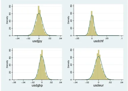
distribution of returns. We will use a histogram to illustrate the density of returns and

11

Figure 1 The distribution of daily exchange rate returns

From Figure1 we see that the returns approximate to a normal distribution. Figure 2 shows that daily log of returns during the time period under study and there are clear periods of volatility clustering.

0 20 40 60 80 D ens it y

-.04 -.02 0 .02 .04

usdjpy 0 20 40 60 80 D ens it y

-.05 0 .05 .1

usdchf 0 20 40 60 80 D ens it y

-.06 -.04 -.02 0 .02 .04

usdgbp 0 20 40 60 80 D ens it y

-.04 -.02 0 .02 .04

12

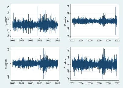
Figure 2 Log of Daily returns

In Figure 2 we can see that that the series are stationary with most of the returns being located around zero. However these some spikes in the first order difference in periods with high volatility. To compare the proposed models we will use the realised volatility which is shown in figure 3:

-.0 4 -.0 2 0 .02 .04 .06 D .us dj py

2002 2004 2006 2008 2010 2012

-.1 -.0 5 0 .05 .1 D .us dc hf

2002 2004 2006 2008 2010 2012

-.0 5 0 .05 D .us dgbp

2002 2004 2006 2008 2010 2012

-.0 4 -.0 2 0 .02 .04 D .us deur

13

Figure 3 Realized volatility

Source Bloomberg

The credit crunch as observed caused a spike in the volatility in all of the exchange rate pairs starting in 2008, the properties of the realised volatility are outlined in Table 1

Table 1: Properties of the realized volatility

Observations Mean Std.Dev Min Max JPY 2609 9.99 3.35 3.24 28.49 CHF 2609 10.95 3.96 4.92 39.30 GBP 2609 9.22 3.77 3.21 30.54 EUR 2609 9.74 3.20 3.93 26.72

From table 1 we see that the swiss franc – dollar parity has both the highest mean of volatility and highest standard deviation, this currency pair also has by far has the largest spread in volatility, much caused by the two spikes in volatility. 0 10 20 30 40 US D/ CHF

2002 2004 2006 2008 2010 2012

5 10 15 20 25 US D/ E UR

2002 2004 2006 2008 2010 2012

0 10 20 30 US D/ G B P

2002 2004 2006 2008 2010 2012

0 10 20 30 US D/ J P Y

14 Figure 4 Implied Volatility

Source: Bloomberg

Figure 3 plots the data on implied volatility. We can see the similarity between the realized and implied volatility. However we see that in case of the swiss franc – dollar parity, the estimated peaks look different for the realized and implied volatility. We can look closer at the properties by putting the data statistics in a table. 5 10 15 20 25 30 US D/ J P Y

01jan2002 01jan2004 01jan2006 01jan2008 01jan2010 01jan2012

5 10 15 20 25 US D/ CHF

01jan2002 01jan2004 01jan2006 01jan2008 01jan2010 01jan2012

5 10 15 20 25 US D/ G B P

01jan2002 01jan2004 01jan2006 01jan2008 01jan2010 01jan2012

5 10 15 20 25 US D/ E UR

15

Table 2: Properties of the implied volatility

Observations Mean Std.Dev Min Max USDJPY 2609 10.50 2.77 6.10 27.39 USDCHF 2609 10.96 2.54 5.52 23.52 USDGBP 2609 9.76 3.25 4.93 24.95 USDEUR 2609 10.71 3.10 5.12 24.65

5. Empirical Results

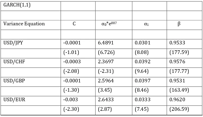
In section, we present results of the in-sample forecast for both the full period and the pre and post commencement of the financial crisis periods. For the GARCH (1,1) model we have four unknown parameters to estimate, namely, 𝐶,𝛼0,𝛼1,𝛽. Estimates were made using MATLAB and are reported it Table 3:

Table 3: Value of GARCH (1,1) parameters for period 2002-12

GARCH(1,1)

Variance Equation C α0*e007 _{α1 β}

USD/JPY -0.0001 6.4891 0.0301 0.9533

(-1.01) (6.726) (8.08) (177.59)

USD/CHF -0.0003 2.3697 0.0392 0.9576

(-2.08) (-2.31) (9.64) (177.77)

USD/GBP -0.0001 2.5964 0.0397 0.9531

(-1.30) (3.45) (8.46) (163.49)

USD/EUR -0.003 2.6433 0.0333 0.9620

(-2.30) (2.87) (7.45) (206.59)

Notes: t-statistics are in parentheses

16

rate pairs on a 1% level. Given the estimated parameters for the variance equations,

ex-post forecasts were carried out (10).

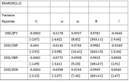
In the EGARCH model an additional parameter has to be estimated in comparison with the standard GARCH model. Since this model is asymmetric, 𝛾 has to be estimated in order to capture the leverage effect. The results are reported in Table 4.

Table 4: Value of EGARCH(1,1) parameters and significance for period 2002-12

We can see from Table 4 that the leverage parameter is not significant at 1% level for pound-dollar and euro-dollar pairs. However the leverage parameter is significant for both the USD/JPY and USD/CHF. Both the ARCH and GARCH parameters are significant on a 1% level for all exchange rate pairs and as in the standard GARCH(1,1) the GARCH parameters are strongly significant (10).

EGARCH(1,1)

Variance

Equation C ω α1 Β γ

USD/JPY -0.0002 -0.2178 0.0927 0.9781 -0.0545

(-2.07) (-6.62) (8.82) (303.11) (-9.45)

USD/CHF -0.004 -0.0145 0.0745 0.9982 -0.0269

(-2.92) (-0.98) (10.61) (663.10) (-5.34)

USD/GBP -0.0001 -0.0773 0.0938 0.9923 0.0058

(-1.09) (-3.61) (9.20) (481.07) (1.91)

USD/EUR -0.0002 -0.0398 0.0743 0.9959 0.0040

(-2.22) (-2.37) (7.45) (601.41) (1.67)

17

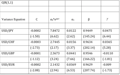
As with EGARCH, modelling the GJR-GARCH model requires estimation of, γ to capture the leverage effect, the results are reported in Table 5

Table 5: GJR-GARCH (1,1) parameter estimates for period 2002-12

GJR(1,1)

Variance Equation C

α0*e007 _{α1 β} γ

USD/JPY -0.0002 7.8472 0.0122 0.9449 0.0475

(-1.50) (6.62) (2.62) (145.24) (6.44)

USD/CHF -0.0003 2.7445 0.0156 0.9634 0.0365

(-2.73) (2.17) (3.37) (202.14) (5.28)

USD/GBP -0.0001 2.3673 0.0441 0.9546 -0.0110

(-1.12) (3.24) (7.66) (166.22) (-1.81)

USD/EUR -0.0002 2.1432 0.0369 0.9629 -0.009

(-2.08) (2.94) (6.53) (207.74) (-1.73)

Note t-statistics in parantheses

From Table 5 we can see that the leverage parameter is significant at the 1% level for yen-dollar and swiss franc dollar parities but only significant at the 10% level for yen-pound-dollar and euro- dollar parities. The GARCH and ARCH parameters are significant at the 1% level. We see that the leverage parameter is negative for pound-dollar and euro-dollar parity, indicating that the relationship between returns and volatility is negative. However, the leverage parameter is allowed to be negative as long as 𝛼1 +𝛾 ≥0, which is the case. In addition the following constraints that 𝛼0 > 0,𝛼1 > 0, 𝛽 ≥0 are all are satisfied in our case.

18

the leverage coefficient as between the EGARCH and GJR models. In the EGARCH model given by equation (5) the model the γ parameter estimates are directly connected to the actual innovations. While in the GJR model, given by equation (7), the leverage coefficient is connected through an indicator variable (I). So when an asymmetric shock occurs, the leverage effect should be negative for the EGARCH model and positive for the GJR model.

19

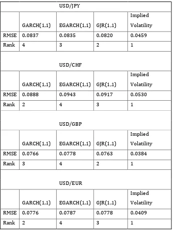
Table 6: Root Mean Squared Error of GARCH and Implied

Volatility Forecasts for the period 2002-2012

USD/JPY

GARCH(1,1) EGARCH(1,1) GJR(1,1)

Implied Volatility

RMSE 0.0837 0.0835 0.0820 0.0459

Rank 4 3 2 1

USD/CHF

GARCH(1,1) EGARCH(1,1) GJR(1,1)

Implied Volatility

RMSE 0.0888 0.0943 0.0917 0.0530

Rank 2 4 3 1

USD/GBP

GARCH(1,1) EGARCH(1,1) GJR(1,1)

Implied Volatility

RMSE 0.0766 0.0778 0.0763 0.0384

Rank 3 4 2 1

USD/EUR

GARCH(1,1) EGARCH(1,1) GJR(1,1)

Implied Volatility

RMSE 0.0776 0.0787 0.0778 0.0409

Rank 2 4 3 1

20

outperformed by the implied volatility forecasts which suggests that the foreign exchange markt is efficient. Indeeed, the implied volatility are significantly below the GARCH estimates for all four currencies studied.

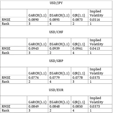
It is well known from previous studies that in periods of high volatility, the GARCH models tend to significantly underestimate volatility. As such, it is important to compare the forecasts in periods with high and low volatility. For this reason, we have divided the data into two sub periods, the pre-financial crisis period 2002-7 and the post-financial crisis period 2008-12. The results of the in sample forecasting exercise is shown in Tables 7 and 8.

Table 7: Root Mean Squared Error for one-step-ahead in-sample forecasts

2002-2007

USD/JPY

GARCH(1,1) EGARCH(1,1) GJR(1,1) Implied Volatility RMSE 0.0890 0.0895 0.0873 0.0516

Rank 3 4 2 1

USD/CHF

GARCH(1,1) EGARCH(1,1) GJR(1,1) Implied Volatility RMSE 0.0943 0.0939 0.0961 0.0413

Rank 3 2 4 1

USD/GBP

GARCH(1,1) EGARCH(1,1) GJR(1,1) Implied Volatility RMSE 0.0774 0.0779 0.0778 0.0375

Rank 2 4 3 1

USD/EUR

GARCH(1,1) EGARCH(1,1) GJR(1,1) Implied Volatility RMSE 0.0849 0.0848 0.0850 0.0373

21

As can be seen in table 7 that there is not a dominant in-sample forecaster among the GARCH models. However, the GJR model is now the least accurate forecast in total. This is the opposite compared to the full period in-sample forecast in section. The implied volatility forecast still outperforms all three GARCH models suggesting that the foreign exchange market efficiency hypothesis .

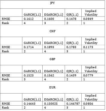
We turn our attention to the period 2008-2012 which is related to periods with greater uncertainty and instability in the financial markets. The volatility is generally at a much high level, and volatility clustering appears in all the exchange rate series .The in-sample forecasts for the period 2008 to end 2012 are reported in Table 8.

Table 8: Root Mean Squared Error for one-step-ahead in-sample forecasts

2008-2012.

JPY

GARCH(1,1) EGARCH(1,1) GJR(1,1) Implied Volatility

RMSE 0.1612 0.1600 0.1478 0.0849

Rank 4 3 2 1

CHF

GARCH(1,1) EGARCH(1,1) GJR(1,1) Implied Volatility

RMSE 0.1714 0.1893 0.1783 0.1173

Rank 2 4 3 1

GBP

GARCH(1,1) EGARCH(1,1) GJR(1,1) Implied Volatility

RMSE 0.1523 0.1562 0.1439 0.0779

Rank 3 4 2 1

EUR

GARCH(1,1) EGARCH(1,1) GJR(1,1) Implied Volatility

RMSE 0.14643 0.150025 0.146787 0.0856

22

Table 8 shows the performance of the GARCH models during the period after the commencement of the financial crisis which was characteried by higher exchange rate volatility. During this time-period the GARCH models are significantly less accurate and the implied volatility forecasts are also less satisfactory compared to the pre risis period. Npnethless the implied volatility forecasts are significantly better than the GARCH models suggesting continued foreign exchange market pricing of options even in periods of high volatility. However is should be remembered as Nelson (2009) points out that implied volatility forecasts can themselves be far from optimal.

In sum, we can see that the GARCH models do not fit the data well in periods of higher volatility. We see how more accurate the models fit the data in the period before the credit crunch. However we observe that this is also the case for the implied volatility. In the first period, the implied volatility is a very good predictor, however, in the high volatility period the implied volatility forecast performs significantly less well in predicting the true volatility.

6. Conclusions

This study shows that GARCH models are not particularly useful in forecasting foreign exchange volatility in periods of either low or high volatility. This can be seen in that none of our three models come close to fitting the data as well as the implied volatility. By contrast, the implied volatility forecasts outperform the GARCH models by a significant amount in both the low and high volatility periods.

23

come close to being a competitor to the superior information contained in implied volatility.

Typically one of the objectives of foreign exchange rate policy has been to iron out “excessive volatility”, but if the foreign exchange market is efficiently pricing in volatility as our results tend to suggest, then from a policy perspective this suggests that the need to intervene to iron out exchange rate volatility is reduced. By efficiently pricing in future prospective volatility currency options provide a means for companies to effectively hedge volatility.

Another policy implication of the market efficiently pricing in volatility is that speculators provide a stabilising influence on the foreign exchange market. Since speculators can buy or sell volatility through currency options which are efficiently priced, then policy makers should worry less about their role in determining exchange rates. Indeed there is a danger that the introduction of a “Tobin tax” on foreign exchange transactions could interfere with the efficiency and price discovery process in the foreign exchange market.

Areas for further research could involve the use of alternative models such as the AP-GARCH specification. Another possibility would be to move away from univariate models to the use of multivariate GARCH models, see for example, Silvennoinen (2008) incorporating independent macroeconomic variables, such as interest rates, fiscal indicators, current account balances, money supplies and government expenditure. Another approach could be that taken by Bildirici, and Ersin (2011) who suggest supplementing GARCH models with the use of neural networks to improve their forecasting ability.

In this study, we have analysed volatility using daily closing prices to perform ex-post forecasts. It would be interesting to use higher frequency data to see whether the results reported in this paper extend to forecasting intra-day volatility.Authors such as Chen et al (2011) have shown that combining a variety of GARCH models and use of intra day data can provide useful information for

24 Footnotes

(1) A symmetric model means that when a shock occurs, we will have a symmetric response of volatility to both positive and negative shocks. Asymmetric models on the other hand, allow for an asymmetric response with empirical results show that negative shocks will lead to higher volatility than a positive shock.

(2) Overfitting happens when the statistical model describes a random error or noise instead of the underlying relationship, causing biasedness in parameter estimates.

(3) The leverage effect where it is typically interpreted as a negative correlation between lagged negative returns and volatility.

(4) As with the EGARCH the GJR-GARCH model captures the leverage effect but the way that it acts is not the same as for the EGARCH, The GJR-GARCH does not measure log returns, so in this model we still need to impose non-negative constraints.

(5) We observe that the difference between ARCH and GARCH is the last term that makes the model less likely to break the non-negativity constraint.

(6) If the restriction does not hold we will have non-stationarity in the variance, if 𝛼1+𝛽 = 1, we have a unit root in the variance.

(7) If 𝛾 = 0, the model is symmetric. There is no need to be concerned about the conditional variance being negative since 𝑙𝑛(𝜎_𝑡2) is modelled.

(8) Bollerslev et al (2001) argue that this type of volatility is an unbiased and very efficient estimator of return volatility.

(9) It should be noted that the parameters (𝛼+𝛽) were less but close to unity, suggesting that the shocks are highly persistent and die out only gradually.

25 References:

Andersen, T. and Bollerslev, T. (1998), DM-Dollar Volatility: Intraday Activity

Patterns, Macroeconomic Announcements, and Longer-Run Dependencies, Journal of

Finance, vol.53, no 1, pp.219-265.

Andersen, T., Bollerslev, T., Diebold, F. And Labys, P. (2001) The Distribution of

Realized Exchange Rate Volatility, Journal of the American Statistical Association, vol 96, no 453, pp.42-55

Andersen, T., Bollerslev, T., Diebold, F.X. and Labys, P. (2003) Modeling and

Forecasting Realized Volatility, Econometrica, 71,no 2, p. 579-626.

Baillie, R. And Bollerslev, T. (1991) Intra-Day and Inter-Market Volatility in Foreign

Exchange Rates, Review of Economic Studies, vol 58, no 3, pp.565-585.

Balaban, E. (2004) Comparative forecasting performance of symmetric and

asymmetric conditional volatility models of an exchange rate, Economic Letters, vol

83, no 1, pp.99-105.

Bildirici M., and Ersin O., (2009). Improving forecasts of GARCH family models

with the artificial neural networks: An application to the daily returns in Istanbul

Stock Exchange, Expert Systems with Applications, vol 36, no 4, pp.7355-7362.

Bollerslev, T. (1986) Generalized Autoregressive Conditional Heteroscedasticity,

Journal of Econometrics, vol 31, no 3, pp.307-327

Bollerslev, T. (2008) A Glossary of ARCH (GARCH), Creates Research Paper,

2008-49.

Brownlees, C. and Gallo, M. (2010) Comparison of Volatility Measures: A Risk

Management Perspective, Journal of Financial Econometrics, vol 8, no 1, pp.29-56.

Busch T, Christensen B, Neilsen M (2012),

Chen, X, Ghysels, E. and Wang, F. (2011). HYBRID GARCH models and Intra-Daily

26

Donaldson, R and Kamstra M (2005) Volatility Forecasts, Trading Volume and the

ARCH vs Option Implied Volatility Tradeoff, Journal of Financial Research, vol 27

no 4, pp.519-538.

Dunis, C., Laws, J. and Chauvin, S. (2003). FX volatility forecasts and the

informational data for volatility. European Journal of Finance, vol 17, no 1, pp.

117-160.

Engle, R. and Patton A., (2001) What is a good volatility model? Quantitative

Finance, vol 1, no 2, pp.237-245.

Ghysels, E. Santa-Clara, P and Valkanov, R. (2005) Predicting volatility: getting the

most out of return sampled at different frequencies. Journal of Econometrics. vol 131,

no 1, pp.59-95.

Glosten, L., Jagannathan, R. and Runkle, D (1993) On the relation between expected

value and the volatility of the nominal excess return on stocks. Journal of Finance, vol

48, no 5, pp.1779-1801.

Hansen, P. and Lunde, X. (2005) A Forecast Comparison of Volatility Models: Does

Anything Beat a GARCH(1,1). Journal of Applied Econometrics, vol 20, no 7,

pp.873-889.

Higgins, M. and Bera, A.(1992). A class of nonlinear ARCH models. International

Economic Review, vol 33, no 1, pp.137-158.

Neely, C. (2009). Forecasting Foreign Exchange Volatility: Why is Implied Volatility

Biased and Inefficient? And Does it Matter? Journal of International Financial

Markets, Institutions and Money, vol 19, no 1, pp.188-205.

Nelson, (1991), ‘Conditional heteroskedasticity in asset returns: A new approach’,

Econometrica 59, no 2, pp.347—370.

Ranaldo, A., (2008), Segmentation and Time-of-Day Patterns in the Foreign

27

Silvennoinen, A and Terasvirta, T (2008). Multivariate GARCH models. In T.G.

Andersen, Davis, Kreiss and Mikosch, eds, Handbook of Financial Time Series, New

York, Springer.

Taylor, S. (1986), Modelling Financial Time Series, Wiley, Chichester.

Zakoïan, J. (1994), “Threshold Heteroskedastic Models,” Journal of Economic

Dynamics and Control, vol 18, no 5, pp.931-955.