City, University of London Institutional Repository
Citation
:
Gorea, A., Belkoura, S. and Solomon, J. A. (2014). Summary statistics for size over space and time. Journal of Vision, 14(9), 22.. doi: 10.1167/14.9.22This is the published version of the paper.
This version of the publication may differ from the final published
version.
Permanent repository link:
http://openaccess.city.ac.uk/15375/Link to published version
:
http://dx.doi.org/10.1167/14.9.22Copyright and reuse:
City Research Online aims to make research
outputs of City, University of London available to a wider audience.
Copyright and Moral Rights remain with the author(s) and/or copyright
holders. URLs from City Research Online may be freely distributed and
linked to.
Summary statistics for size over space and time
Andrei Gorea
Universit ´e Paris Descartes & CNRS, Paris, FranceLaboratoire Psychologie de la Perception,$
Seddik Belkoura
Universit ´e Paris Descartes & CNRS, Paris, FranceLaboratoire Psychologie de la Perception,$
Joshua A. Solomon
Optometry Division, Applied Vision Research Centre,City University London, UK#
$
A number of studies have investigated how the visual system extracts the average feature-value of an ensemble of simultaneously or sequentially delivered stimuli. In this study we model these two processes within the unitary framework of linear systems theory. The specific feature value used in this investigation is size, which we define as the logarithm of a circle’s diameter. Within each ensemble, sizes were drawn from a normal distribution. Average size discrimination was measured using ensembles of one and eight circles. These circles were presented simultaneously (display times: 13–427 ms), one at a time, or eight at a time (temporal-frequencies: 1.2–38 Hz). Thresholds for eight-item ensembles were lower than thresholds for one-eight-item ensembles. Thresholds decreased by a factor of 1.3 for a 3,200% increase in display time, and decreased by the same factor for a 3,200% decrease in temporal
frequency. Modeling and simulations show that the data are consistent with one readout of three to four items every 210 ms.
Introduction
Within the framework of linear systems theory, the temporal impulse response (TIR) can be considered a primitive, from which several psychophysical results evolve. In general, the TIR describes visual activity following a briefly presented stimulus. When that stimulus is a luminance grating that has a relatively high spatial frequency, the TIR is biphasic (De Lange,
1952; Gorea & Tyler, 1986). Low-frequency gratings produce monophasic TIRs (Kelly, 1977).
Contrast thresholds can be predicted from the total visual activity, during and after each presentation. For relatively short presentations, Bloch’s Law (Bloch,
1885) says that the product of contrast threshold and
duration should be a constant. Adherence to Bloch’s Law is not always perfect (Gorea & Tyler, 1986; Watson, 1986). When we refer to empirically derived functions mapping presentation durations of arbitrary length to performance threshold, we will use the more general term Bloch’s Curve.
Bloch’s Law also has implications for speeded-response detection tasks: Response time at constant performance should be inversely proportional to the stimulus intensity. Over the last three decades or so, this paradigm has become popular for investigating how sensory evidence is accumulated over time. Alternative to linear systems theory are drift-diffusion models, which stipulate that the evidence for and against the presence of a visual signal should be encoded in terms of its likelihood (or log-likelihood; Gold & Shadlen, 2001; Bogacz, Brown, Moehlis, Holmes, & Cohen, 2006; Yang & Shadlen, 2007). While this latter class of models provides good fits to
behavioral (e.g., Usher & McClelland, 2001; de
Gardelle & Summerfield, 2011) and physiological (e.g., Gold & Shadlen, 2001; Yang & Shadlen, 2007)
decision-time data, the proposal that the brain inte-grates log-likelihood ratios rather than stimulus strength remains debatable (e.g., Liston & Stone, 2013).
The temporal contrast sensitivity function (TCSF) is another empirically derived curve. It maps the recip-rocal of contrast threshold (i.e., sensitivity) to temporal frequency. Linear systems theory describes how this function can also be predicted from the TIR. The two types of curve are related by the Fourier Transform (De Lange, 1952; Kelly, 1977). Thus, there is a sound theoretical basis for predicting two types of empirical results from the temporal impulse response: Bloch’s curve and the TCSF.
In this paper we measure Bloch’s curve and the TCSF in an effort to characterize the evidence
Citation: Gorea, A., Belkoura, S., & Solomon, J. A. (2014). Summary statistics for size over space and time.Journal of Vision,
accumulation process supporting the extraction of summary statistics, specifically the mean size of a set of items. Once all items in a set have reached (and exceeded) their detection threshold (an assumedly parallel process), estimates of summary statistics may be refined over time in a continuous manner, just as in the drift-diffusion models of detection (Ratcliff,1978; Gold & Shadlen, 2001; Usher & McClelland, 2001; Bogacz et al., 2006; Brunton, Botvinick, & Brody, 2013) or their linear-systems equivalents (Watson, 1979, 1986; Gorea & Tyler, 1986, 2013).
Data relevant to the accumulation of summary statistics were collected by Chong and Treisman (2003), who found a rather modest benefit of exposure durations longer than 50 ms. However, without formal modeling, it remains unclear whether there wasn’t more benefit because observers had already integrated all the avail-able evidence before 50 ms had elapsed, or whether they simply didn’t use much of the available evidence in the first place. Monte Carlo simulations were provided later by Myczek and Simons (2008), who concluded it was possible that no more than two circles were ever used in a computation of mean size. Problems with these simula-tions include a lack of parameters for coding noise, decision noise, and the explicit relationship between exposure duration and the number of circles used in a computation (Ariely, 2008). Whether Chong and Treis-man’s (2003) observed slight performance improvement with duration was due to observers using more items in their estimates of the mean, an increase in their acuity for size (equivalent to a decrease in coding and/or decision noise), or both remains an open question.
Below, we answer this question by fitting Bloch’s curve and the TCSF with the noisy, inefficient observer model of Solomon, Morgan, and Chubb (2011).
Furthermore, we present an elaboration of that model, in which responses are based on the accumulated evidence from a series of independent, parallel measurements. Of particular interest is the frequency with which the putative parallel measurements can be made, and how that frequency compares with other cognitive processes.
Finally, we acknowledge limitations with this class of models, such as their equal treatment of all inputs (cf. de Gardelle & Summerfield,2011), and we examine our own data for evidence that certain circles are given greater weighting in decisions about average size.
Methods
Participants
Five graduate students (age range: 19–23, including author SB) and author AG participated in all duration
and temporal frequency (Main) experiments. The same two authors and one of the other graduate students also participated in an experiment (hereafter referred to as the Noise Experiment) where the mean-size dis-crimination thresholds were assessed as a function of size variance. All participants had normal or corrected-to-normal vision.
Stimuli
The stimuli were presented using a Dell Precision T3500 computer (Dell, Round Rock, TX) on a 19-in. E96fþSB ViewSonic monitor (1280·1024 pixels, 75 Hz; ViewSonic, Walnut, CA) set at about 60 cm from observers’ eyes. Stimuli presentation and response recording were implemented in Matlab using the Psychophysics Toolbox (Brainard, 1997; Pelli, 1997).
Stimuli were white (44 cd/m2) or black (0.05 cd/m2)
circle outlines (five-pixel width) presented on a gray
background (22 cd/m2). Their polarity was changed
systematically across trials to avoid possibly con-founding stimulus exposure with luminance adapta-tion. Their contrast was such that even under the shortest display durations and the highest temporal frequencies they were highly suprathreshold. A white central cross was used for fixation. The screen was partitioned into two hemifields by a black, three-pixels thick vertical line.
Main Experiments
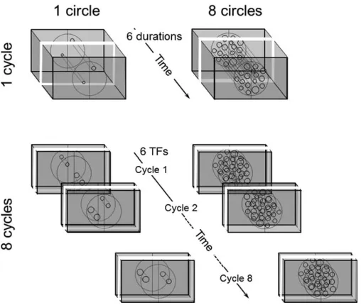
The circles were presented on each side of this vertical line either one or eight per hemifield and either once or repeated eight times per trial. When presented only once per trial their exposure duration could take one of six durations (T: 13.3, 26.7, 53.3, 106.6, 217.3, and 426.5 ms). When repeated they were refreshed at one of six Temporal Frequencies (TF: 1.17, 2.3, 4.7, 9.4, 18.8, and 37.5 Hz) with a 0.5 duty-cycle. Eight temporal cycles were always presented so that the total duration of a flickering trial depended on TF. The TFs were chosen so that the duration of one-half temporal cycle at the highest frequency equaled the shortest once-per-trial condition. At the lowest frequency it equaled the longest durations used in the once-per-trial condition. When presented only once per trial, the number of circles per hemifield (Ns) was either 1 or 8. When presented repeatedly in one trial each temporal cycle also displayed 1 or 8 elements. Hence, there were 2 ·2 experimental conditions, hereafter referred to as 1:1, 1:8, 8:1, and 8:8 (i.e., Ns:Nt; see Appendix 1 for a
diameters were randomly drawn from one of two
lognormal distributions, either lnN[l-Dl/2;r2
Cor
lnN[lþDl/2;r2
C. 1
In this experiment the parameter
controlling stimulus variance was fixed atrC¼0:2.
This is the largest value used by Solomon et al. (2011).
The baselinelwas itself a random variable drawn
across trials from a flat distribution, such thatl[1.18,
2.78]. The ratioDl/l was under the control of two
staircases per experimental condition (see Procedure). One or eight circles’ locations were randomized both across trials and temporal cycles. These locations were constrained such that (a) circles were always within a
circular area around fixation with a 138 radius and (b)
the outlines of the simultaneously presented circles
were always at least 18 apart.
Noise Experiment
This experiment was in all respects equivalent to the Main Experiment with two exceptions. In the first phase only condition 8:1 (eight circles presented once) was tested, and for only two display durations (13.3 and 426.5 ms). Mean-size discrimination thresholds were measured for six levels of the parameter control-ling stimulus variance,rC. These levels were equally
spaced on a log axis between 0.01 and 0.50. To accommodate the largest variances and ensure that all
circles could be contained within the appropriate hemifield, the range of baseline diameters was reduced to [1.18, 1.98]. The second phase was identical to the first, except only the 1:1 condition was tested, and only two levels of rCwere used: 0.01 and 0.20.
Procedure
The order of the four Main conditions (1:1, 1:8, 8:1, 8:8) was randomized across participants. The different timings of the stimuli, their color (white or black), their locations, and their baseline diameter lwere random-ized across trials. The participant’s task was to decide which of the two hemifields contained the circle(s) with the largest mean size (a two alternative forced-choice paradigm). Participants indicated their response by pressing one of two keys. There was no feedback. The expected size difference between circles in the left and right hemifields was under the control of two inter-leaved staircases (accelerated stochastic approximation algorithm; Kesten, 1958) set to converge on a
performance of 81%for each experimental condition so
that there were 12 interleaved staircases per experiment and per session. Typically, each staircase converged
after an average of about 25 trials. Five trials withDl/l
well beyond the discrimination threshold (or just-noticeable Weber fraction) were randomly interspersed among each staircase trials to assess the percentage of lapses. Each participant first ran one training session with condition 1:8 (at least 120 trials). The four conditions were repeated four times in a random order
so that each hwas computed as the geometric mean of
four assessments. The whole experiment was completed in about 3 hrs typically dispatched in two or three sessions per day.
The Noise Experiment was run once all Main Experiments were completed. As a result, only three of the original participants were still available. The procedure was in all respects identical to that described above with the exception that this time the two durations and the up to six stimulus variances were randomized across sessions and participants. The experiment was completed within about 1 hr (no breaks).
Results
Main Experiments thresholds
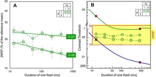
Figure 2A shows the mean-size discrimination
thresholds (h·100%) averaged over all six observers as
[image:4.612.40.294.58.273.2]a function of the display duration for conditions 1:1 (circles) and 8:1 (squares) (all symbols and notations are summarized in Appendix 1). Thresholds drop with
duration but the slopes of the linear regressions (in log-log coordinates; straight lines) are very shallow, congruent with a statistical summation process (see the
Modeling section): The slope for condition 1:1 is0.03,
which is not significantly different from 0 (F¼2.08,p¼
0.158); the slope for condition 8:1 is0.08, which is
significantly different from 0 (F¼4.67,p¼0.037).2 It
should be pointed out that a threshold drop with duration is theoretically obligatory due to an inevitable reduction of early noise (see also The generalized NIO model section).
Overall, mean-size discrimination thresholds for one single circle are 1.4 times higher than for eight
simultaneously displayed circles. An ideal observer should have decreased its thresholds by a factor offfiffiffi
8
p
¼2.83. The lesser summation assessed in human observers may be caused by their coding and decision noise and by their lesser coding efficiency (see the Modelingsection). When compared with the contrast detection thresholds in the standard Bloch’s Law regime over the same duration range (Figure 2B, shaded area) they appear to be almost independent of duration. While over the same duration range contrast detection thresholds for low and high spatial frequen-cies (upper and lower continuous curves) drop by respectively 0.47 and 0.82 log-units (the pairs of red closed circles on each curve), mean-size discrimination thresholds drop by only 0.12 log-units.
Figure 3A shows the mean-size discrimination
sensitivity (1/[h ·100]) averaged over the six observers
as a function of the display TF for conditions 1:8 (circles) and 8:8 (squares). Here again, sensitivity barely
varies with TF. When compared with the standard Temporal Modulation Transfer functions for contrast (Figure 3B) over the same TF range they show a maximum modulation of 0.23 log-units, while the maximum sensitivity modulation for low and high spatial frequencies is 2.5 and 2.8 log-units (pairs of red closed circles on the left and right smooth curves, respectively).
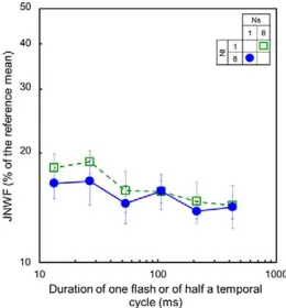
Figure 4 displays the 8:1 data from Figure 2A together with the 1:8 data from Figure 3A with the later now plotted as a function of the duration of half a cycle of the respective TFs. This is the duration for which each refreshed circle is continuously visible over the eight cycles of the flickering stimuli. The observation here is that the amount of summation over eight spatially or temporally distributed items is (close to)
equivalent (two-way repeated measures ANOVA, F[1,
71]¼0.98,p¼0.32).3 This is true independently of the
rate (TF) at which size information is delivered
(interaction: F[5, 71]¼0.11,p¼0.99).
Noise Experiment thresholds
Figure 5 shows size discrimination thresholds (h ·
100) of three observers (different symbols) for condi-tion 8:1 and stimulus duracondi-tions of 13 and 427 ms (open and solid symbols, respectively) as a function of the parameter controlling stimulus variance. This figure suggests that duration has a large effect on threshold when stimulus variance is low; it has little effect on threshold when stimulus variance is high.
Figure 2. (A) Mean-size Just Noticeable Weber Fractions (JNWF) averaged over the six observers as a function of stimulus duration for conditions 1:1 and 8:1 (open circles and squares, respectively). Straight lines are linear regression fits with slopes of0.03 and0.08. (B) The same data (open symbols in the shaded area) rescaled to match the scale of the standard Bloch’s Law plots for low and high spatial frequencies (continuous top and bottom curves, respectively; adapted with permission from Gorea & Tyler,1986). The pair of red closed circles on each curve shows the highest and lowest thresholds within the display duration range tested in the present experiments. Vertical bars in each panel are61 SE.
Figure 3. (A) Mean-size sensitivity (1/JNWF) averaged over the six observers as a function of TF for conditions 1:8 and 8:8 (closed circles and squares, respectively). (B) The same data (closed symbols in the shaded area) rescaled to match the scale of standard Temporal Modulation Transfer Functions (TMTFs) for low and high spatial frequencies (left and right curves, respectively; adapted with permission from Gorea & Tyler,
[image:5.612.40.293.61.186.2] [image:5.612.317.572.61.189.2]Modeling
The Noise Experiment thresholds are useful for disentangling two qualitatively different limitations in performance. One type of limitation is inefficiency. An inefficient observer may base his judgments on the median size instead of the mean. Or, if there is a mode, maybe he uses that. Or he may even calculate the mean size, but not of all the circles. In other words, an inefficient observer makes the wrong calculation. Nonetheless, he makes that calculation perfectly. A different kind of limitation is imprecision. The impre-cise observer may indeed calculate the geometric mean of all diameters, but—like virtually all measurements— there will be some variability in his calculation; he won’t get the same value every time. These different types of limitation have different effects on the ‘‘hockey-stick’’ (Allard & Cavanagh,2012) function mapping log stimulus standard deviation to log threshold (see Figure 5). Increasing imprecision raises the left-hand branch. Increasing inefficiency always elevates the right-hand branch. Its effect on the left-hand portion depends on the source of imprecision.
The noisy, inefficient (but otherwise ideal)
observer model
In Solomon et al.’s (2011) parameterization of the noisy, inefficient observer (NIO) model, sources of imprecision are either ‘‘early’’ (i.e., independently affecting each item in an ensemble) or nominally ‘‘late’’ (i.e., affecting the decision variable). When, as in these experiments, the lapse rates are virtually zero, Solomon et al.’s equation 4 implies that the size-discrimination threshold can be modeled as
h¼exp U1ð0:81Þ
ffiffiffiffiffiffiffiffiffiffiffiffiffiffiffiffiffiffiffiffiffiffiffiffiffiffiffiffiffiffiffiffiffi
r2 Lþ
2ðr2 Eþr2CÞ
M r
" #
1: ð1aÞ
For convenience, we used the following approxima-tion.
h’U1ð0:81Þ
ffiffiffiffiffiffiffiffiffiffiffiffiffiffiffiffiffiffiffiffiffiffiffiffiffiffiffiffiffiffiffiffiffi
r2 Lþ
2ðr2 Eþr2CÞ
M
r
: ð1bÞ
In the foregoing expressions,U1 is the inverse standard normal distribution, (0.81 was the conver-gence point of the adaptive staircases), r2
C is the
parameter controlling stimulus variance, andr2 E;r
2 Land
M are free parameters. The first two are the variances of the early and late noises, respectively, and M is the effective maximum number of circles used by observers to compute the mean of each array of Nselements (M Ns). A random perturbation with variancer2E is
added to the effective size of each item independently, while a random perturbation with variancer2
Lis added
to the difference between estimates of the sample mean effective sizes. Note that segregating the cause of imprecision into an early and late stage is somewhat arbitrary. If, instead of late noise, we allow the random perturbation added to the effective sizes of any two elements to have correlation q, then we can reparame-terize Equation 1b such that
h’U1ð0:81Þ
ffiffiffiffiffiffiffiffiffiffiffiffiffiffiffiffiffiffiffiffiffiffiffiffiffiffiffiffiffiffiffiffiffiffiffiffiffiffiffiffiffiffiffiffiffiffiffiffiffiffiffiffiffiffiffiffi
2qðM1Þ
M r
2 Eþ
2ðr2 Eþr2CÞ
M r
: ð1cÞ
[image:6.612.368.525.59.145.2]For each observer and each duration, we simulta-neously fit the NIO model to the data from two conditions: 1:1 (not shown for better legibility) and 8:1 (dashed and solid curves in Figure 5for 13- and 427-ms
[image:6.612.100.230.60.200.2]Figure 4. Mean-size JNWF for condition 8:1 (squares; from Figure 2A) together with the thresholds for condition 1:8 (circles; from Figure 3A) with the latter now plotted as a function of the duration of half a cycle of the temporally modulated stimuli (instead of their TF).
stimulus presentations). The fits minimized the root-mean-squared (RMS) log error between the model’s predictions and the measured thresholds. There were
three free parameters in each fit:r2
E;r 2
L, andM. In these
fits efficiency and precision were constrained to be nondecreasing with exposure duration. Thus we
ensuredM427ms M13ms, r2E;427ms r2E;13ms, and
r2
L;427msr2L;13ms. Like Solomon et al. (2011) we, too,
found sizeable individual differences in efficiency, with observer SB effectively using 5.9 circles in his calcula-tions and observer HV effectively using just 3.7 (see inset in Figure 5). Notably, however, the present data suggest virtually zero effect of exposure duration on
efficiency (averageM¼5). On the other hand, exposure
duration does seem to affect all observers’ precision (either early noise, late noise, or both).
The generalized NIO (gNIO) model
gNIO development
Time is not a variable in Solomon et al.’s (2011) NIO model. However, if observers could accumulate evi-dence during the course of a trial, it is conceivable that efficiency and/or precision might increase with dura-tion. We modelled evidence accumulation as the result of series of independent, parallel measurements of circle size. In the present generalization of the NIO, parallel
measurements ofmcircles in each hemifield occur
within a putative ‘‘attentional loop’’. Equation 1b can be considered a special case (see below) of this gNIO:
h¼U1ð0:81Þ ffiffiffiffiffiffiffiffiffiffiffiffiffiffiffiffiffiffiffiffiffiffiffiffiffiffiffiffiffiffiffiffiffiffiffiffiffiffiffiffiffiffiffiffiffiffiffiffiffiffiffiffiffiffiffiffiffiffiffiffiffiffiffiffiffiffiffiffiffiffiffiffiffiffiffiffiffiffiffiffiffiffiffiffiffiffiffiffiffiffiffiffiffiffiffiffiffiffir2 Lþ2NCðrC2;l;m;Ns;NtÞ þ2NEðr2e;l;m;Ns;NtÞ
q
ð2Þ
whereNCðr2
C;l;m;Ns;NtÞ and NEðr2e;l;m;Ns;NtÞ
rep-resent the (necessarily independent) contributions of the stimulus and early noise to the variance of estimated averages (i.e., one on each side of the
display), respectively. Note that when the symbolNhas
a capital subscript, it denotes a variance (in squared units of what Solomon et al., 2011, call ‘‘effective size’’); when it has a lower-case subscript, it denotes a number (i.e., of either elements or pairs of subarrays).
Each variance is as a function of: Ns, the number of simultaneously visible elements within each of these subarrays; Nt, the number of successively exposed subarrays on each side of the display;l, the number of times (a.k.a. ‘‘loops’’) an observer forms an indepen-dent estimate using the same subarray;m, the
maximum effective sample size of each aforementioned independent estimate. As with Solomon et al. (2011), we consider a circle’s effective size to be proportional to its diameter’s logarithm. The remaining two symbols in
Equation 2 arer2
e, which describes the variance of an
early noise that is added to the effective size of each
item independently on each loop, andr2
L, which
describes the variance of a late noise that is added to the difference between estimates of sample mean effective sizes. Note that in the gNIO model, responses
are based on the average of l ·Nt independent
estimates. Each estimate is based on up to 2·mcircles
(mon the left plusmon the right). If fewer than 2·m
circles appear during the loop, then that loop’s estimate is based on the number of circles that did appear. It doesn’t matter whether these elements are there for the whole loop or not (the understanding being that, once they exceed the detection threshold, their sizes are instantaneously coded). Instead, the shorter the loop,
the higher the best-fittingr2
e will be. The derivation of
NCand NE is developed in Appendix 2.
gNIO fit
To fit our data with the generalized NIO (or gNIO), we assumed that the number of loops (l) per subarray would be proportional to the duration of each subarray. Thus the full gNIO has four free parameters: m, re, rL, and l13. The first three
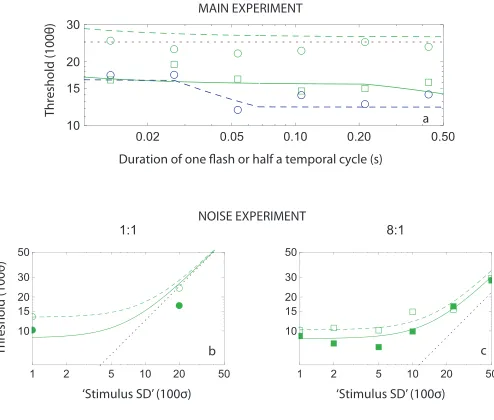
parameters are defined in the preceding section. The fourth parameter is the number of loops during the shortest stimulus exposure (13.3 ms). The gNIO was fit to the geometric mean thresholds from the three observers (AG, HV, and SB) who participated in both the Main Experiment and the Noise Experiment. (The Main Experiment alone was insufficient to constrain all four parameters.) Best-fitting parameter values were: m¼3.2, re¼0.02, rL¼0.10, and l13¼0.0625. The RMS error between the model’s predictions and 34 datum points (18 from the Main Experiment, omitting 8:8,4 plus 16 from the Noise Experiment) was 0.05 log units. These fits and the corresponding datum points are shown in Figure 6. Note that 0.0625 loops per 13.3 ms yields a loop duration of 213 ms, i.e., about two loops for the present longest presen-tation duration.
There are several notable features of the fit. For example, there seem to be some cases in which human observers outperform the ideal: Some empty green circles (condition 1:1) fall below the dotted magenta line in Figure 6a and one symbol (filled green circle) falls below the dotted black line in Figure 6b. Since better-than-ideal performance is impossible, the dis-tances between these symbols and the ideal lines provide some indication of the large measurement error in these conditions. However, since these datum points cannot be well-fit whatever the values of the models’ parameters, they could not have influenced the best-fitting parameter values.
frequencies lower than 19 Hz. Givenl13¼0.0625, this is
the point at which exactly one loop extends over the eight cycles. Below this frequency the gNIO is able to
use more thanm elements from each hemifield. At
0.068 s per half-cycle (7 Hz), the number of loops
during each cycle becomes 1/mand thus the gNIO is
able to use all the circles in its computations (see Equation A5 and related text in Appendix 2). This feature of the fits provides a strong constraint on the duration of each loop, such that there is a well-defined minimum in the function mapping parameter values to the RMS error (Figure 7). It is partially supported by the statistical analysis mentioned in Footnote 3, even though no such significant difference is observed when considering the data of all six observers (see Figure 4 and related analysis). This apparent discrepancy may be accounted for by the fact that the goodness-of-fit statistics (RMS) for our model fits decreases only mildly for loops longer than 200 ms so that our loop-duration estimate allows for some variability.
Regression weights
In experiments where observers had to discriminate the mean-shape and mean-color of sets of 12 items presented simultaneously, de Gardelle and Summerfield
(2011) derived the regression weights of the ranked
shapes and colors in each sample and found signifi-cantly larger weights for items whose critical features (shape or color) were closer to the mean feature of the sample. They referred to such weighting as ‘‘robust’’ in the sense that it minimizes the contribution of outliers. However, an ideal observer gives equal weights to all
magnitudes of a sample of items providedthat these
weights are applied to the effectivemagnitudes of the
attribute under consideration (e.g., luminance, con-trast, size, shape, etc.). By effective we mean the
physical valuetransducedby the brain (frequently
referred to as the psychophysical function, i.e., the function that expresses the relationship between the physical magnitude of a stimulus and the magnitude of the sensory response evoked by that stimulus; Fechner, 1858).
[image:8.612.344.549.59.189.2]Once the physical magnitudes are transformed by the psychophysical function, they should all count equally in the observer’s computation. An analysis suggesting unequal contributions of the presented magnitudes to the computation of their mean (such as in de Gardelle & Summerfield,2011) implies that the magnitudes used in the derivation of the corresponding weights were obtained via an incorrect psychophysical function (including constant or linear functions). Using a log transformation of diameter and a logistic regression analysis equivalent to that used by de Gardelle and Summerfield (2011), we obtained size-rank weights (for conditions 8:1 and 8:8) not significantly different from constant. This suggests that our log transform is close to the psychophysical function for size, but given the large confidence intervals about all derived weights, we cannot be certain this is the case. As the inference of the
Figure 6. Fits of the gNIO model to geometrically averaged duration dependent thresholds for all three observers who participated in both the Main Experiment (condition 8:8 excluded, panel a) and the Noise Experiment (panels b and c for conditions 1:1 and 8:1, respectively). In panel a, empty green circles and squares and empty blue circles represent the measured thresholds for conditions 1:1, 8:1, and 1:8, respec-tively. Dashed green, solid green, and dashed blue lines are gNIO model fits to these data. The dotted magenta line represents the ideal observer’s thresholds in the 1:1 condition (ideal thresholds for 8:1 and 1:8 conditions are less than 10). In panels b and c, open and solid symbols (data) and dashed and solid curves (fits) represent thresholds for 13.3 ms and 427 ms presentations, respectively, for conditions 1:1 (circles) and 8:1 (squares) with the dotted straight black lines showing the performance of the ideal observer.
[image:8.612.43.290.60.270.2]size-transducer was not one of the goals of this study, we did not pursue this line of analysis.
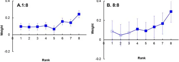
More interesting is the weighting of the sizes as a function of their temporal order in conditions 1:8 and 8:8. These temporal order weights were derived using a logistic regression procedure (Ludwig, Gilchrist, McSorley, & Baddeley,2005; de Gardelle & Summer-field, 2011) applied either to the difference between log diameters (condition 1:8) or to the difference between the average log diameters (condition 8:8) in the two hemifields (Figure 8).
The temporal order coefficients displayed in Figure 8
show a general tendency to increase with their rank. This tendency is statistically significant for both (1:8 and 8:8) regressions. Also, the first three coefficients for condition 8:8 are not significantly different from 0 implying that the first three (out of eight) frames were not considered in computing the average size. Overall one may conclude that late frames in a temporal sequence are more heavily weighted than early frames (a recency effect; Ebbinghaus, 1913).
The recency effect
The recency effect revealed by the larger weights given to late items in a temporal sequence is tanta-mount to an imperfect memory, which can be modeled as a leaky temporal integration (Ossmy, Moran, Pfeffer, Tsetsos, Usher, & Donner,2013; Usher & McClelland, 2001). It is reasonable to assume that such an increase in weighting over time should also occur over successive attentional loops. This possibility was not considered in the gNIO model where memory was taken to be perfect, i.e., where the computation of means over loops was leakless. One possible imple-mentation of such leakage is in terms of a Markov-like memory process where the previously estimated mean and the current evidence are given different weights in the computation of the current estimate. A tentative modeling of the recency effect with such a Markov-like process could not simultaneously account for the data obtained with 1.2 and 37 Hz stimulus presentations
while keeping the duration of the attentional loop constant. As a consequence it has not been incorpo-rated in the gNIO model.
Discussion
The main results of the present study are as follows: (a) The mean size of a set of eight items (circles) is computed with a precision that increases by a factor of about 1.3 (0.11 log-units) over a display duration range spanning a factor of 32 (1.5 log-units; from 13.3 to 426.5 ms), translating into a slope (in a log-log space) of 0.08 significantly different from 0 (p¼0.04). (b) An even shallower slope (0.03), marginally different from 0 (p¼0.15), was observed for estimating the size of one single item over the same duration range. (c) Increasing the sample size from one to eight items increases size discrimination sensitivity (one/threshold) by an average factor of 1.4, while an ideal observer should have increased it by a factor of pffiffiffi8¼2.83. (d) Mean-size discrimination sensitivities for one and eight items repeatedly presented for eight temporal cycles drops when their temporal frequency increases from 1.2 to 37.5 Hz (·32) by factors of at most·1.2 and·1.8 (for one and eight items, respectively), much less than expected from a linear integration process and pretty much in line with Haberman, Harp, and Whitney’s
(2009) results for averaging sequentially presented
faces. (e) For these two sequentially distributed conditions (one and eight items repeatedly presented), mean-size discrimination sensitivities differ by an
average factor of about 1.15 (instead of pffiffiffi8¼2.83 for
[image:9.612.150.462.62.171.2]the ideal observer). (f) Finally, the present data show that the integration of eight items over space or over time (simultaneously and sequentially presented, re-spectively) yields about identical mean-size discrimi-nation thresholds. This comparison might not be fully warranted. Contrary to the continuous presentation (condition 8:1), in the sequential condition (1:8) the actual duration of each flicker frame might have included a remnant of which observers (who definitely
did not report it) might have taken advantage. On the other hand, items on each but the last frame in a sequence might have been masked by the items in the following frame (even though not presented at the very same locations). This being said, the fact remains that under the present stimulating conditions observers integrate information over space and over time with about equal efficiency.
In short, our data show close to null mean-size computation dependency on the temporal factors of the stimuli presentation. In that, our data agree with all the published studies including those having reported an accuracy dependency on display duration (Chong & Treisman,2003; Whiting & Oriet, 2011) or on reaction times (Robitaille & Harris, 2011). The apparent incongruence between some of these reports and the present data comes from these studies (a) not having related the accuracy improvement with the range of display durations (or of reaction times) and/or (b) having assessed accuracy in terms of percent correct rather than in threshold units (Robitaille & Harris, 2011; Whiting & Oriet, 2011) and/or (c) having used rather intricate experimental designs some of which included a backward mask without specifying the visibility of the stimuli for the shortest displays (Robitaille & Harris, 2011). The present data also clearly show that observers use more than one item in a sample of eight (whether simultaneously or sequentially presented), as the discrimination thresholds are signif-icantly lower for samples of eight items than for samples of one item. (See also Piazza, Sweeny, Wessel, Silver, & Whitney, 2013, for an equivalent conclusion in an auditory summary statistics experiment.) Such improvement is substantially less than it should have been, had observers used all eight items with maximum efficiency.
The data were analyzed in two different ways. We first fit Solomon et al.’s (2011) ‘‘noisy, inefficient (but otherwise ideal) observer’’ (NIO) model to three observers’ discrimination thresholds, measured as a function of the variability of the displayed elements, to
derive observers’ internal (early,rE, and late,rL) noise
andtotalefficiency,M. As this model does not include
a stimulus duration parameter,rE andM refer to the
noise and efficiency over the whole inspection period. The fit of the NIO model did yield, as expected, a
smallerrEfor the longest (427 ms) than for the shortest
(13 ms) stimulus duration (rE,13ms¼0.10,rE,427ms¼
0.047; averaged over observers) but also a small
unexpectedrLdrop over this same time span (from
0.11 to 0.08 when averaged over observers) even though these drops were not systematic across observers. The fits did show an effect of exposure duration on efficiency, but only for one of the three observers (see inset in Figure 5).
We developed a generalized version of the NIO model (gNIO) to include a time factor conceptualized as a time-limited attentional loop, with its associated sample size m. During such a loop the early noise NE decreases with time but the subsample mremains the same, with a new m-subsample being drawn with replacement on each new loop. When best-fit to the data, the duration of each loop was 213 ms (i.e., ;5 Hz), with an effective sample size per loop (m) of 3.2 items. The gNIO model (Equation 2) fits best with 3
m 4, definitely larger than 1 or 2 as suggested by
Myczek and Simon’s (2008) noiseless simulations. Of particular interest is the inferred 5-Hz loop frequency which is within the range of attentional sampling, as inferred by a number of authors from similar (1–8 Hz; Wyart, de Gardelle, Scholl, & Summerfield, 2012) and entirely different experiments (4–10 Hz; e.g., Rullen, Carlson & Cavanagh, 2007; Busch & Van-Rullen, 2010; Macdonald, Cavanagh, & VanVan-Rullen, 2014).
Previous research has demonstrated that contrast is integrated linearly over time up to about 30 ms (Gorea & Tyler, 1986). Our stimuli had highly suprathreshold contrasts, and thus their visibility was presumably independent of the display duration. Consequently, the present results suggest that the size averaging operation is time dependent because the system cannot take in all the available information at once. Our modeling suggests that information may be accumulated in attentional loops, whose number increases as time goes by. The increase of the information and the decrease in noise with the number of loops are of statistical nature. Together they yield only a very shallow increase in sensitivity with stimulus exposure time: a factor of 1.3
for a 3,200%increase in presentation time. As a
system’s temporal integration behavior is directly related (via its temporal impulse response) to its temporal contrast sensitivity function (see Introduc-tion), the latter should also be little dependent on the temporal frequency of the stimulus presentation (as presently observed).
This scenario is very much akin to Gorea and Tyler’s
(1986) account of the contrast integration process for
durations beyond linear integration and beyond the temporal probability summation regime (Watson, 1979). According to Gorea and Tyler’s modeling (see their equation 6 and their figure 4), the contrast temporal impulse response constrains linear integration (i.e., linear filtering) within a window of about 30–50 ms. Beyond that duration integration is nonlinear, reflecting either probability summation (within a
high-threshold formulation) or a hard-wired nonlinearity (b
’ 4) followed by nonprobabilistic linear summation.
inferred duration of one attentional loop. Sensitivity
(i.e.,di0) is computed within each second-order window
(i), with the total, time-dependent sensitivity given by
the sensitivity summation rule,d0¼
ffiffiffiffiffiffiffiffiffiffiffiffiffiffiffiffiffiffiffiffiffi
Pn
i¼1ðd
0
iÞ
2
q
(Green & Swets, 1966). Beyond the second-order integration regime sensitivity improves with duration with a log-log
slope of1/2b¼ 0.125 (see equation 10 in Gorea &
Tyler, 1986), not so far from the presently observed
slope of0.08. The favorable comparison of the
present modeling parameters with those of Gorea and Tyler’s linear systems approach strongly suggests that humans’ temporal integration behavior for higher-level visual tasks (such as the extraction of summary statistics) can be reasonably described within the framework of the linear systems theory.
Following a number of recent studies (Ludwig et al.,
2005; de Gardelle & Summerfield, 2011; Wyart et al., 2012; Brunton et al., 2013), we also examined the weights given by the averaging process to the different sizes in a sample, and to the different temporal
positions of sequentially presented items. A logistic regression analysis revealed insignificantly different size-rank weights but a statistically significant tendency to more weighting the later three frames in a sequence of eight. The apparent discrepancy between the robust averaging in de Gardelle and Summerfield’s (2011) study for shape and color and the present more or less equal weighting for size could be due to the different transducers subserving the different perceptual dimen-sions. As the psychophysical function is definitely unknown for the shape and color dimensions and as it remains debatable for the size dimension (see Teght-soonian, 1965; see also Footnote 1) the comparison between our inferred size weights and the inferred weights by in de Gardelle and Summerfield (2011) for shape and color is pointless.
The presently observed recency effect (also docu-mented in Tsetsos, Chater, & Usher,2012) is at odds with the nonmonotonic weighting over time found for 40-Hz sequential presentations of luminance blobs in an average luminance discrimination task (Ludwig et al., 2005). It is also different from the constant temporal weighting derived for trains of randomly timed light pulses (4.5 Hz) and auditory clicks (20, 40 Hz) in a counting discrimination task (Brunton et al., 2013), and for an orientation averaging task with stimuli delivered at 4 Hz (Wyart et al., 2012). Critical differences across these four studies (type of stimuli— e.g., masked vs. not masked—and their temporal characteristics, magnitude of the samples and their variance, task type, and modeling approach) may well account for such discrepancies (see Tsetsos et al., 2012; Ossmy et al., 2013). Be it as it may, a tentative modeling of the present recency effect as a Markovian process could not simultaneously account for the data obtained with 1.2- and 37-Hz stimulus presentations
while keeping the duration of an attentional loop constant. Integrating other available recency effect models (such as those pertaining to limitations of short term memory, to temporal distinctiveness, or to contextual variability; see for a review Howard & Kahana, 2002) within our gNIO is a task for the future.
Conclusion
The present experiments and modeling within the framework of linear systems theory suggest that in a mean-size discrimination task observers compute the mean size by effectively subsampling about four items at a time out of the total number of items presented and repeat such subsampling with replacement at a
frequency of about 5 Hz for as long as the stimulus is present. This process yields a very small performance improvement over time. Applying linear system theory to higher level visual processes appears to be a
modeling approach not less valid than the drift diffusion modeling approach.
Keywords: visual size discrimination, spatio-temporal integration, efficiency, linear systems theory, attentional loops
Acknowledgments
Authors AG and JAS were supported by Royal Society grant IE111227. Author SB was supported by a scholarship from the Institute of Neuroscience and Cognition of Universit´e Paris Descartes. AG designed research; SB performed research and analyzed data; JAS modeled the data; AG and JAS wrote the paper.
Commercial relationships: none. Corresponding author: Andrei Gorea. Email: [email protected].
Address: Laboratoire Psychologie de la Perception, Universit´e Paris Descartes & CNRS, Paris, France.
Footnotes
1Weber’s Law for diameter (Solomon et al.,2011)
models (e.g., the Noisy Inefficient Observer [NIO] and generalized NIO [gNIO]) –see the corresponding sections in the paper– are difficult to reconcile with the magnitude estimation (Teghtsoonian, 1965; Chong & Treisman, 2003), because the latter suggest expansive transduction of circle diameters. Therefore, we have decided to reserve further attempts to reconcile magnitude estimation with discriminability for future discussion.
2For the three observers who also completed the
Noise Experiment (which constrained fits of the gNIO, see below), the slopes of the linear regressions (in log-log coordinates) for conditions 1:1 and 8:1 are, respectively,0.022 and0.043, neither of which is significantly different from 0.
3
For the three observers who also completed the Noise Experiment (which constrained fits of the gNIO, see below), ANOVA suggests a marginally significant difference,F(1, 35)¼2.83,p¼0.105.
4
As described inAppendix 2 (see Equations A11 and A12), Monte Carlo simulations were required to estimate the contribution of stimulus noise to
discrim-ination. We tried all combinations ofm(up to 8) andl
(up to 8) for the condition 8:1, in which the
aforementioned contribution would be constant
when-ever there were fewer than one loop per subarray (i.e.,l
,1). Simulations are much more complicated for
condition 8:8, because the aforementioned contribution is no longer constant when, as our data with short displays and high temporal frequencies suggest, there are fewer than one loop per subarray.
References
Allard, R., & Cavanagh, P. (2012). Different processing strategies underlie voluntary averaging in low and high noise.Journal of Vision, 12(11):6, 1–12, http:// www.journalofvision.org/content/12/11/6, doi:10. 1167/12.11.6. [PubMed] [Article]
Ariely, D. (2008). Better than average? When can we say that subsampling of items is better than statistical summary representations? Perception & Psychophysics, 70(7), 1325–1326, discussion 1335– 1336, doi:10.3758/PP.70.7.1325.
Bloch, M. A. (1885). Experiments in vision (transla-tion). Comptes Rendus de Se´ances de La Socie´te´ de Biologie, Paris, 37(2), 493–495.
Bogacz, R., Brown, E., Moehlis, J., Holmes, P., & Cohen, J. D. (2006). The physics of optimal decision making: A formal analysis of models of performance in two-alternative forced-choice tasks.
Psychological Review,113(4), 700–765, doi:10.1037/ 0033-295X.113.4.700.
Brainard, D. H. (1997). The Psychophysics Toolbox.
Spatial Vision, 10, 433–436.
Brunton, B. W., Botvinick, M. M., & Brody, C. D. (2013). Rats and humans can optimally accumulate evidence for decision-making. Science, 340(6128), 95–98, doi:10.1126/science.1233912.
Busch, N. A., & VanRullen, R. (2010). Spontaneous EEG oscillations reveal periodic sampling of visual attention. Proceedings of the National Academy of Sciences, USA, 107(37), 16048–16053, doi:10.1073/ pnas.1004801107.
Chong, S. C., & Treisman, A. (2003). Representation of statistical properties. Vision Research,43(4), 393– 404.
De Gardelle, V., & Summerfield, C. (2011). Robust averaging during perceptual judgment.Proceedings of the National Academy of Sciences, USA,108(32), 13341–13346, doi:10.1073/pnas.1104517108.
De Lange, H. (1952). Experiments on flicker and some calculations on an electrical analogue of the foveal systems. Physica, 18(11), 935–950.
Ebbinghaus, H. (1913). On memory: A contribution to experimental psychology. New York: Teachers College.
Fechner, G. T. (1858). U¨ber ein Psychophysisches Grundgesetz [Translation: On a basic psychophys-ical law]. Memoirs of the Leipzig Society, 6, 457– 532.
Gold, J. I., & Shadlen, M. N. (2001). Neural
computations that underlie decisions about sensory stimuli. Trends in Cognitive Sciences, 5(1), 10–16. Gorea, A., & Tyler, C. W. (2013). Dips and bumps: On
Bloch’s law and the Broca-Sulzer phenomenon.
Proceedings of the National Academy of Science, USA, 110(15), E1330.
Gorea, A., & Tyler, C. W. (1986). New look at Bloch’s law for contrast. Journal of the Optical Society of America A, 3(11), 52–61.
Green, D. M., & Swets, J. A. (1966). Signal detection theory and psychophysics. New York: Wiley. Haberman, J., Harp, T., & Whitney, D. (2009).
Averaging facial expression over time. Journal of Vision, 9(11):1, 1–13, http://www.journalofvision. org/content/9/11/1, doi:10.1167/9.11.1. [PubMed] [Article]
Howard, M. W., & Kahana, M. J. (2002). A distributed representation of temporal context. Journal of Mathematical Psychology, 46(3), 269–299, doi:10. 1006/jmps.2001.1388.
Kelly, D. H. (1977). Visual contrast sensitivity. Optica Acta, 24(2), 107–129.
approxima-tion. Annals of Mathematical Statistics, 29(1), 41– 59.
Liston, D. B., & Stone, L. S. (2013). Saccadic
brightness decisions do not use a difference model.
Journal of Vision, 13(8):1, 1–10, http://www. journalofvision.org/content/13/8/1, doi:10.1167/13. 8.1. [PubMed] [Article]
Ludwig, C. J. H., Gilchrist, I. D., McSorley, E., & Baddeley, R. J. (2005). The temporal impulse response underlying saccadic decisions. Journal of Neuroscience, 25(43), 9907–9912, doi:10.1523/ JNEUROSCI.2197-05.2005.
Macdonald, J. S. P., Cavanagh, P., & VanRullen, R. (2014). Attentional sampling of multiple wagon wheels. Attention, Perception & Psychophysics,
76(1), 64–72.
Myczek, K., & Simons, D. J. (2008). Better than average: Alternatives to statistical summary repre-sentations for rapid judgments of average size.
Perception & Psychophysics,70(5), 772–788, doi:10. 3758/PP.70.5.772.
Ossmy, O., Moran, R., Pfeffer, T., Tsetsos, K., Usher, M., & Donner, T. H. (2013). The timescale of perceptual evidence integration can be adapted to the environment.Current Biology,23(11), 981–986, doi:10.1016/j.cub.2013.04.039.
Pelli, D. G. (1997). The VideoToolbox software for visual psychophysics: Transforming numbers into movies. Spatial Vision, 10, 437–442.
Piazza, E. A., Sweeny, T. D., Wessel, D., Silver, M. A., & Whitney, D. (2013). Humans use summary statistics to perceive auditory sequences. Psycho-logical Science, 24(8), 1389–1397, doi:10.1177/ 0956797612473759.
Ratcliff, R. (1978). A theory of memory retrieval.
Psychological Review, 85(2), 59–108.
Robitaille, N., & Harris, I. M. (2011). When more is less: Extraction of summary statistics benefits from larger sets. Journal of Vision,11(12):18, 1–8, http:// www.journalofvision.org/content/11/12/18, doi:10. 1167/11.12.18. [PubMed] [Article]
Solomon, J. A., Morgan, M. J., & Chubb, C. (2011). Efficiencies for the statistics of size discrimination.
Journal of Vision, 11(12):13, 1–11, http://www. journalofvision.org/content/11/12/13, doi:10.1167/ 11.12.13. [PubMed] [Article]
Teghtsoonian, M. (1965). The judgment of size.
American Journal of Psychology,78(3), 392–402. Tsetsos, K., Chater, N., & Usher, M. (2012). Salience
driven value integration explains decision biases and preference reversal.Proceedings of the National
Academy of Sciences, USA, 109(24), 9659–9664, doi:10.1073/pnas.1119569109.
Usher, M., & McClelland, J. L. (2001). The time course of perceptual choice: The leaky, competing accu-mulator model. Psychological Review,108(3), 550– 592, doi:10.1037//0033-295X.108.3.550.
VanRullen, R., Carlson, T., & Cavanagh, P. (2007). The blinking spotlight of attention. Proceedings of the National Academy of Sciences, USA,
104(49), 19204–19209, doi:10.1073/pnas. 0707316104.
Watson, A. B. (1979). Probability summation. Vision Research, 19, 515–522.
Watson, A. B. (1986). Temporal sensitivity. In K. Boff, L. Kaufman, & J. Thomas (Eds.), Handbook of perception and human performance (pp. 6–9). New York: Wiley.
Whiting, B. F., & Oriet, C. (2011). Rapid averaging? Not so fast! Psychonomic Bulletin & Review, 18(3), 484–489, doi:10.3758/s13423-011-0071-3.
Wyart, V., de Gardelle, V., Scholl, J., & Summerfield, C. (2012). Rhythmic fluctuations in evidence accumulation during decision making in the human brain.Neuron, 76(4), 847–858, doi:10.1016/j. neuron.2012.09.015.
Yang, T., & Shadlen, M. N. (2007). Probabilistic reasoning by neurons. Nature,447(7148), 1075– 1080.
Appendix 1:
Main symbols and notations used in the text
d0 Signal Detection Theory index of sensitivity
l Number of times (a.k.a. ‘‘loops’’) an observer forms an independent estimate using the same subarray
M Maximum effective sample size per subarray in the NIO
m Maximum effective sample size per subarray per loop in the gNIO
NC Contribution of stimulus noise to the variance of
estimated averages in the gNIO
NE Contribution of early noise to the variance of
estimated averages in the gNIO
b Shape parameter of the Weibull distribution; a measure of psychometric slope
re Standard deviation of an early noise that is
Ns Number of simultaneously visible circles within each subarray
Nt Number of successively exposed subarrays on each side of the display
h Mean-size discrimination threshold
q Correlation between two samples of early noise in the NIO
rC Standard deviation of stimulus sizes (i.e., log
diameters)
rE Standard deviation of early noise in the NIO
rL Standard deviation of late noise in the NIO and
gNIO
U1Inverse standard normal distribution function NB: Conditions 1:1, 1:8, 8:1, and 8:8 all have the formNs:Nt.
Appendix 2:
The generalized NIO
The generalized NIO (gNIO) model is described by Equation 2in the main text. It includes four free
parameters,r2
L (the variance of a late noise added to
the difference between estimates of sample mean
effective sizes),r2
e (the variance of an early noise
added to the effective size of each item independently
on each loop),l (the number of times or ‘‘loops’’ an
observer forms an independent estimate of the mean
size using the same subarray), andm (the maximum
effective sample size of each such independent
estimate). In the present experiments both Nsand Nt
were either 1 or 8, hence yielding four spatio-temporal combinations 1:1, 8:1, 1:8, and 8:8. These are the last two digits appearing between parentheses in the left side expressions of the equations below.
Sincemis the maximum effective sample size on each
side of the display, it cannot exceed the total number of elements that appear on each side during a single loop. Thus, when there is at least one loop per
subarray, l 1 ) mNs. However, when there is
less than one loop per subarray,mcan be larger than
Ns. In the limit, when all subarrays are exposed within
the same loop,mis bound by the total number of
elements on each side of the array, l 1/Nt ) m
NsNt. Furthermore, we adopt the ‘‘reasonable’’
(Allard & Cavanagh, 2012) assumption that all
estimates are based on at least one element, i.e.,m
1. Consequently,
NCðr2C;1;1;1;1Þ ¼r2C ðA1Þ
and
NEðr2e;1;1;1;1Þ ¼r2e ðA2Þ
Given perfect integration (i.e., perfect memory) of l
independent estimates:
NCðr2C;l;1;1;1Þ ¼r 2
C ðA3Þ
and
NEðr2e;l;1;1;1Þ ¼
r2 e
l ðA4Þ
In the expression above, r2
e gets divided byl in
Equation A4 because the correlation between
succes-sive samples of early noise is 0, but r2
Cdoes notget
divided by l in Equation A3 because the correlation
between successive estimates of the same sample of
stimulus noise is 1.
For arrays having eight successively displayed
elements (i.e., one at a time), the observer will pick up
m of the total available elements on each side during each loop. (This number will be zero on half the total number of loops because elements were presented with a duty cycle of 1/2.) When there is at least one loop per exposure (i.e., l 1), the observer will pick up all eight elements in the array. When all eight exposures occur within the same loop, the observer will only get a total of m on each side. Thus, in general, we have:
NCðr2C;l;m;1;8Þ ¼
r2 C
maxfm;8min 1;f lmgg ðA5Þ and
NEðr2e;l;m;1;8Þ ¼
r2 e
8lm ðA6Þ
For arrays having eight simultaneously displayed
elements, after one estimate (i.e., one loop) we have:
NCðr2C;1;m;8;1Þ ¼
r2 C
m ðA7Þ
and
NEðr2e;1;m;8;1Þ ¼
r2 e
m ðA8Þ
Given l estimates, we have
NEðr2e;l;m;8;1Þ ¼
r2 e
lm ðA9Þ
but the expression for NCðr2C;l;m;8;1Þ becomes
rather complex because the correlation between successive estimates (with efficiencym/8,1) of the same sample is neither 0 nor 1, but something in between, which depends on l andm.
We evaluatedNCð1;l;m;8;1Þfor all combinations of
NCð1;l;m;8;1Þ ¼
1
8 1þ7e
0:490ðl1Þ0:793ðm1Þ
h i
ðA10Þ
was found to produce an excellent fit (R2¼0.983) to these 8·8¼64 values. Consequently,
NCðr2
C;l;m;8;1Þ ¼ r2
C
8 1þ7e
0:490ðmax 1f ;lg1Þ0:793ðm1Þ
h i
ðA11Þ
should be a fairly close approximation, even for noninteger values ofl and m.
For arrays having eight successively displayed subarrays of eight elements each, the observer will pick
upmof the total available elements on each side during each loop. When there is at least one loop per exposure, the contribution of stimulus noise to the variance of estimated averages will be one-eighth of what it was when only one subarray was exposed, i.e.
l1)NCðrC2;l;m;8;8Þ ¼
1 8NCðr
2
C;l;m;8;1Þ
ðA12Þ