City, University of London Institutional Repository
Citation
:
Tsigritis, T. and Spanoudakis, G. (2013). Assessing the genuineness of events in
runtime monitoring of cyber systems. Computers and Security, 38, pp. 76-96. doi:
10.1016/j.cose.2013.03.011
This is the accepted version of the paper.
This version of the publication may differ from the final published
version.
Permanent repository link:
http://openaccess.city.ac.uk/2466/
Link to published version
:
http://dx.doi.org/10.1016/j.cose.2013.03.011
Copyright and reuse:
City Research Online aims to make research
outputs of City, University of London available to a wider audience.
Copyright and Moral Rights remain with the author(s) and/or copyright
holders. URLs from City Research Online may be freely distributed and
linked to.
Assessing the genuineness of events in runtime monitoring of cyber
systems
Theocharis Tsigkritis
aaCrypteiaNetworks, Athens, Greece
Email: Theocttsigkritis@crypteianetworks.com
George Spanoudakis
bbSchool of Informatics, City University London, London, United Kingdom
Email: g.e.spanoudakis@city.ac.uk
Abstract — Monitoring security properties of cyber systems at runtime is necessary if the preservation of such properties cannot be guaranteed by formal analysis of their specification. It is also necessary if the runtime interactions between their components that are distributed over different types of local and wide area networks cannot be fully analysed before putting the systems in operation. The effectiveness of runtime monitoring depends on the trustworthiness of the runtime system events, which are analysed by the monitor. In this paper, we describe an approach for assessing the trustworthiness of such events. Our approach is based on the generation of possible explanations of runtime events based on a diagnostic model of the system under surveillance using abductive reasoning, and the confirmation of the validity of such explanations and the runtime events using belief based reasoning. The assessment process that we have developed based on this approach has been implemented as part of the EVEREST runtime monitoring framework and has been evaluated in a series of simulations that are discussed in the paper.
Keywords — cyber system monitoring, event trustworthiness, belief based reasoning, abductive reasoning
I. INTRODUCTION
Monitoring the preservation of security properties of distributed software systems at runtime is a form of operational verification that complements static or dynamic model checking and system testing. Monitoring is particularly important for security properties in cases where the preservation of the specification of a system by its implementation cannot be guaranteed, or there is a possibility of having runtime interactions between system components, which are difficult to foresee and detect during system design and testing and can create security vulnerabilities. Such circumstances may arise when systems deploy software components outside the ownership and control of the system provider dynamically.
Cyber systems – i.e., systems based on components distributed and deployed over the Internet (and possibly a mix of local area and ad hoc networks) and offering services accessible over it – fall under this category due to the inevitably loose control and distributed ownership of the components that they deploy. Successful security attacks over cyber systems (e.g., denial-of-service attacks, man-in-the-middle attacks), indicate that regardless of how carefully the security of system component interactions and communications has been analysed, it will always be possible to identify system vulnerabilities and lunch successful cyber attacks [51].
Over the last decade, several approaches have been developed to support runtime system monitoring (aka runtime verification). Some of these focus on monitoring security properties (e.g. [18][21][23][26][29][46]) whilst others are aimed at monitoring other general types of system properties (e.g. [5][6][10]). Also when it comes to cyber systems, monitoring tends to focus on the network (as opposed to the application) level [44][45][44][47][48][49].
Figure 1. Location based access control system (LBACS)
To illustrate why, consider a system providing location based access control to different resources of an organisation with spatially distributed premises, based on user and device authentication, as well as device location information; this system is an industrial case study introduced in [3] that we will refer to as “Location Based Access Control System” or simply “LBACS” in the following. In LBACS, users who move within the distributed physical spaces of the organisation using mobile computing devices (e.g., PDAs, smart phones) may be given access to different resources (e.g., intranet, printers, scanners), depending on their credentials, the credentials of their devices, and their exact location within the physical space(s). Such resource accessing scenarios arise frequent in systems supporting digital commercial and financial transactions (e.g., systems with mobile points of sale, mobile banking etc.) as well as enterprise systems allowing and/or based on bring your own device (BYOD) scenarios [50].
Fig.1 shows the components and physical configuration of LBACS. As shown in the figure, the operation of LBACS is based on several autonomous and distributed components. These include a location server, an access control server, sensors and Internet routers. The access control server polls the location server at regular intervals, to obtain the position of the devices of all the users who are logged on to LBACS. LBACS compliant devices can log on to it through the wireless network available in the physical space controlled by LBACS (not the sensors) and must have installed daemons sending signals to the location server via the location sensors, periodically. Based on these signals, the location server can calculate the position of a device at regular time intervals. Note that LBACS components may be distributed across different physical spaces (e.g., office spaces and hardware/software components may be located in different buildings).
The correctness and security of the operation of LBACS depends on several conditions including, for example, the liveness of daemons in the mobile devices, the confidentiality of signals sent from daemons to the location server, and the availability of the location server. Such conditions need to be monitored at runtime, as attacks to LBACS components can compromise the whole system operation. However, as the components of LBACS are autonomous, runtime checks need to be based on some external monitoring entity receiving and checking events emitted from LBACS components. Furthermore, to ensure that the results of the monitoring process are correct, it is necessary to assess whether the runtime events received by the monitor are trustworthy, faulty, or the result of an attack onto the system. Delayed or dropped signals from the daemons of mobile devices would, for instance, prevent the detection of the location of a device and lead to not allowing it to access certain resources. Also, an attack resulting in delaying or dropping the signals of the location server can compromise the whole operation of LBACS, preventing access to any resource controlled by it.
As discussed earlier, runtime monitoring has been supported by several approaches and systems. However, to the best of our knowledge, the problem of assessing the trustworthiness of events that underpin the monitoring process, in cases of cyber systems like LBACS, has received less attention in the literature.
The process of generating explanatory hypotheses is based on abductive reasoning [30]. Following the generation of hypothetical explanations for an event, we assess their validity by identifying the effects that the generated explanations would have if they were correct, and checking whether these effects correspond and can, therefore, be confirmed by other runtime events in the monitor’s log.
It should be noted that the exploration of violations of desired system properties has been the focus of work in software engineering (e.g., [6][15][31][37]) and AI (e.g., [11][32]) and has been often termed as “diagnosis”. In this work, diagnosis is typically concerned with the detection of the root causes of violations or faults through the identification of the trajectories of events that have caused them. This is similar to the work that we present in this paper. However, the focus of our approach is different from existing work on diagnosis, since our focus is the assessment of the trustworthiness of the events that indicate the presence of violations of desired system properties as opposed to the identification of the root cause of a detected system fault or security violation (see Sect VI for a more detailed comparison).
To cope with inherent uncertainties that arise in assessing the trustworthiness of monitoring events, the assessment of the validity of the explanations generated for the events and the event trustworthiness itself is based on the computation of beliefs using belief measuring functions grounded in the Dempster-Shafer (DS) theory of evidence [33]. The belief-based assessment of event trustworthiness becomes what we term in our approach as “event genuineness”.
To test and validate our approach, we have developed an event assessment module as part of the Event Reasoning Toolkit (EVEREST [35][36]). EVEREST has been developed to support the monitoring of security and dependability properties for distributed systems expressed as monitoring rules in a formal temporal logic language that is based on Event Calculus (EC) [22], called EC-Assertion.
Early versions of our event assessment approach have been presented in [39][40][41]. The main contributions of this paper with respect to our earlier work are related to:
(a) the introduction new belief functions for assessing event genuineness and the formalisation of these functions in the context of the DS theory of evidence;
(b) the introduction of the algorithm for generating hypothetical explanations of events;
(c) the explanation of how the results of the diagnosis process can be utilised in monitoring; and (d) the experimental evaluation of our approach.
The rest of this paper is organised as follows. Section II provides background information regarding the EVEREST framework that underpins the implementation of our approach. Section III presents the process of generating and validating event explanations. Section IV describes the belief functions used to assess event genuineness. Section V presents an experimental evaluation of our approach. Section VI overviews related work. Finally, Section VII provides some concluding remarks about our approach and outlines plans for further work.
II. PRELIMINARIES:THE EVEREST FRAMEWORK
Before discussing the details of our approach, we provide an overview of the EVEREST system and the way in which it expresses the properties to be monitored. This is necessary in order to understand the form of the diagnosis model used by our approach.
A. Overview of EVEREST
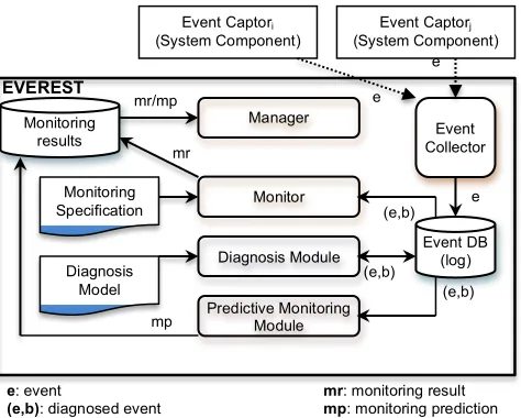
Fig. 2 shows the overall architecture of EVEREST, which consists of an Event Collector, a Monitor, a Predictive Monitoring Module, a Manager and a Diagnosis Module (i.e., the module implementing the approach that we describe in this paper).
The event collector receives notifications of events that are captured by external captors, transforms these events into an internal representation used by EVEREST, stores the transformed events into an internal event database (aka monitor log), and notifies other EVEREST components that events have occurred.
The monitor checks if the received events violate specific properties. This module is implemented as a reasoning engine whose operation is driven by the monitoring specification provided for a system. This specification consists of monitoring rules expressing the properties that need to be checked at runtime and monitoring assumptions that are used to set and update the values of state variables required for monitoring. Monitoring rules and assumptions are expressed as EC-Assertion formulas as discussed in Section II.B.
Figure 2. EVEREST architecture
The assessment of the genuineness of runtime events is the responsibility of the diagnosis module of EVEREST. The module generates explanations of runtime events based on a diagnosis model of the system under surveillance and uses them to compute beliefs in the trustworthiness of events. These beliefs are then stored in the event database (Event DB) from which they can be accessed by the monitor and the predictive monitoring module. The diagnosis model used in this process contains assumptions about the operation of the system under surveillance. These assumptions take the form of sequences of operation invocations and responses as well as the effect that these actions have in the state of the system (see Sect III.B below for examples).
The monitor and the predictive monitoring module store their results in a monitoring results database (Monitoring Results DB), along with diagnostic information regarding the genuineness of the events that have caused a violation or underpin the prediction about a violation. This database is accessed by the Manager, which provides an interface to external clients for retrieving detected violations for a given system. B. Monitoring specifications and diagnostic models
In EVEREST the properties to be monitored are expressed as formulas of EC-Assertion [35]. EC-Assertion is a restricted form of the first order temporal logic language of Event Calculus (EC) [22].
[image:5.595.161.398.79.269.2]The basic modeling elements of EC are events and fluents. An event is something that occurs at a specific instance of time and is of instantaneous duration. The occurrence of an event at a particular instance of time is expressed by the predicate Happens. Events may change the state of the system that is being modeled. More specifically, an event can initiate or terminate a state. States are modeled as fluents and the initiation and termination of a fluent by an event are expressed by the predicates Initiates and Terminates, respectively. In addition to the predicates Happens, Initiates and Terminates, EC offers the predicate HoldsAt which expresses a check of whether a given fluent holds at a specific instance of time.
TABLE I. EC-ASSERTION PREDICATES & THEIR MEANINGS
Predicate Meaning
Happens(e,tℜ(tL,tU)) An event e of instantaneous durations occurs at some time point t within
the time range ℜ(tL,tU) (
ℜ(tL,tU)=[ tL,tU]).
HoldsAt(f,t) A state (aka fluent) f holds at time t. This is a derived predicate that is true if the f has been initiated by some event at some time point t’ before t and has not been terminated by any other event within the range [t’,t].
Initiates(e,f,t) Fluent f is initiated by an event e at time t Terminates(e,f,t) Fluent f is initiated by an event e at time t Initially(f) Fluent f holds at the start of system operation.
<rel>(x,y)
where <rel>::= = | < | > | ≤ | ≥ | ≠
The relation <rel> holds between the x and y.
EC-Assertion adopts the basic modeling constructs of EC but introduces special terms to represent types of events, fluents and computations needed for runtime monitoring, and special predicates to express comparisons between basic data type values (see [35] for more details), and terms denoting calls to special built-in functions that are available in order to compute complex computations (e.g. to compute statistical
Predictive Monitoring Module Diagnosis Module
Event Collector
EVEREST
Monitor
Event Captorj
(System Component)
Manager
Event DB (log) Monitoring
results
e e
(e,b) e Event Captori
(System Component)
Monitoring Specification
Diagnosis
Model (e,b)
e
mr: monitoring result mp: monitoring prediction e: event
(e,b): diagnosed event
(e,b) mr
information and fit statistical distributions over data). The exact syntactic form and meaning of the predicates Happens, Initiates, Terminates, HoldsAt and Initially in EC-Assertion are shown in Table I.
The properties monitored by EVEREST are expressed in EC-Assertion as monitoring rules of the form mr: B1∧ … ∧ Bn⇒ H1∧ … ∧ Hm.
In this form, the predicates Bi and Hj are restricted to Happens, HoldsAt and relational predicates. A
monitoring rule mr is satisfied if when the sub formula B1∧ … ∧ Bn (aka body of the rule) becomes True, the
sub formula H1∧ … ∧ Hm (aka head of the rule) also becomes True.
An example of an EVEREST monitoring rule is given below: Monitoring Rule R11
Happens(e(_eID1,_devID,_locServerID, REQ, signal(_devID),_locServerID), t1, R(t1,t1)) ⇒
Happens(e(_eID2,_devID,_locServerID, REQ, signal(_devID),_locServerID), t2, R(t1,t1+m)) ∧ _eID1 ≠ _eID2
This rule refers to the LBACS system introduced in Sect. I and checks the liveness of daemons in the mobile devices accessing LBACS. In particular, R1 checks if the location server of LBACS (signified by the value of the variable _locServerID) receives signals from a given device (_devID) every m time units. Every signal that is sent by a device and captured by the location server at some time point t1 will trigger the check
of the rule by matching the predicate
Happens(e(_eID1,_devID,_locServerID,REQ,signal(_devID),_locServerID),t1,R(t1,t1)) in the body
of the rule. Subsequently, the monitor of EVEREST will expect to receive another signal (event) from the same device that could be matched with the predicate Happens(e(_eID2,_devID, _locServerID,REQ,signal(_devID),_locServerID),t2,R(t1,t1+m)) at some time point t2 that is within
the range [t1, t1+m] and if no such a signal is received the rule will be violated.
Another example of a monitoring rule of LBACS is: Monitoring Rule R2:
Happens(e(_eID1,_devID,_ctrlServerID, REQ,
requestAccess(_devID,_result),_ctrlServerID), t1,R(t1,t1)) ⇒ HoldsAt(AUTHENTICATED(_devID),t1)
This rule checks if a device has been authenticated when it makes a request to the control server for accessing a resource. The authentication of a device that sends the request is indicated by the fluent AUTHENTICATED(_devID) and the rule checks the authentication through the predicate HoldsAt(AUTHENTICATED(_devID),t1). As discussed earlier, however, HoldsAt is a derived predicate that is true only if its fluent argument has been initiated by an event prior to the time at which the predicate is checked and has not been terminated by any other event until then. Thus, when the monitor receives a resource access request event matching the Happens predicate in its body (i.e., a requestAccess(_devID,_result) event) at some time point t1, it will need to check if the HoldsAt
predicate in its head is true at the same time.
Since, in EC fluents can only be initiated and terminated by events, the monitoring specification in this instance will need to specify how the fluent AUTHENTICATED(_devID) is initiated and (if applicable) terminated. In EVEREST, this is specified by monitoring assumptions. A monitoring assumption in EC-Assertion has the form : B1∧ … ∧ Bn⇒ H1∧ … ∧ Hm where predicates Bi are restricted to Happens, HoldsAt
and relational predicates and the predicates Hj are restricted to Initiates and Terminates predicates.
In the case of R2 the monitoring assumption used to establish how AUTHENTICATED(_devID) is initiated is:
Monitoring Assumption MA1
Happens(e(_eID2,_ntwrkCntrl,_devID, RES, connect(_devID,
_connection),_ntwrkCntrl), t1, R(t1,t1)) ∧ (_connection ≠ NIL) ⇒ Initiates( e(_eID2, …), AUTHENTICATED(_devID), t1)
According to this assumption, a device is authenticated if it has made a request for connection to the controller of the network in the area covered of LBACS at least once (see the event connect(_devID, _connection) and this request has been accepted (as specified by _connection ≠ NIL) .
It should be noted that the general form of monitoring assumptions of EVEREST that was shown above allows the expression of more complex patterns of fluent initiation and termination than the pattern shown in
the previous example. The monitoring assumption MA2 below gives an example of a fluent that is used to record movements of a device in different parts of the network of the LBACS case study (i.e., the fluent MOVEMENT(_devID,_originalNetworkController,_destinationNetworkController)). As indicated by MA2, when a device makes two consecutive requests for connection to two different areas of the LBACS network, the fluent MOVEMENT is initiated to indicate the movement of the device between these two areas.
Monitoring Assumption MA2
Happens(e(_eID1,_ntwrkCntrl1,_devID, REQ, connect(_devID, _connection1),_ntwrkCntrl1), t1, R(t1,t1)) ∧
Happens(e(_eID2,_ntwrkCntrl2,_devID, REQ, connect(_devID, _connection2),_ntwrkCntrl2), t2, R(t1,t2)) ∧
(_ntwrkCntrl1 ≠ _ntwrkCntrl2) ∧
¬∃t3: Happens(e(_eID3,_ntwrkCntrl3,_devID, REQ, connect(_devID, _connection3),_ntwrkCntrl3), t3, R(t3,t3)) ∧ (t3 ≤ t1) ∧ (t3 ≤ t2) ⇒ Initiates( e(_eID2, …), MOVEMENT(_devID,_ntwrkCntrl1,_ntwrkCntrl2),t2)
To assess the trustworthiness of events, EVEREST relies on a diagnostic model (see Fig. 1). This model consists of diagnostic assumptions about the system under surveillance.
Diagnostic assumptions are specified as EC-Assertion formulas of the form a: B1∧ … ∧ Bn⇒ H. In this
form, Bi can be any of the EC predicates shown in Table I, and H can be a Happens, Initiates or Terminates
predicate. HoldsAt predicates cannot be specified in the head (H) of diagnostic assumptions since their truth-value can only be derived from the axioms of EC. Diagnostic assumptions enable the specification of expected sequences of events, which may be observable events (i.e., events of the system under surveillance that are visible to the monitor) or internal events of the system under surveillance. Internal events are events that might not be desirable to emit externally (e.g. due to performance or confidentiality reasons) but are often necessary to include in a diagnostic model in order to indicate how a system operates internally. The following formula gives an example of a diagnostic assumption for LBACS:
Diagnostic Assumption DA1
Happens(e(_eID1,_x1,_x2, activeDaemon(_devID),_x3),t1,R(t1,t1))⇒
(∃t2:Time)Happens(e(_eID2,_devID,_locSerID, signal(_devID),_locSerID), t2, R(t1,t1+2))
DA1 states that if the daemon of a device is active at a given time point t1, then it must send a signal to the
location server within 2 time units. As we discuss in Sect. IV below, this assumption enables the diagnosis process to create a hypothesis (explanation) that the daemon of a device, which appears to have sent a signal to the location server of LBACS, was active for a given period before the dispatch of the signal.
III. ASSESSMENT OF EVENT GENUINENESS
A. Overview
The event assessment process has three phases: (i) the explanation generation phase in which hypotheses about the possible explanations of events are generated; (2) the effect identification phase in which the possible consequences (effects) of the hypothetical explanations of an event are derived; and (3) the explanation validation phase in which the expected consequences of each explanation are checked against the event log of the monitor to establish if there are events that match the consequences and, therefore, provide supportive evidence for the validity of the explanation.
The above phases are described in detail below. B. Generation of event explanations
The first phase of the assessment process uses abductive reasoning to find possible explanations for events. The algorithm used to carry out this process is shown in Fig. 3.
The algorithm gets as input an atomic predicate e for which an explanation is required and the boundaries of the time range of this predicate tmin(e) and tmax(e). It also has a fourth input parameter, called finit,
can be assumed through the abduction process), a pair of the predicate e and its time range (i.e., (e, tmin(e),
tmax(e))) is added to the current list of explanations Φe and the algorithm terminates by returning Φe (see lines
[image:8.595.121.435.114.522.2]8 and 44 in Fig. 3).
Figure 3. Explanation generation algorithm
If e is not an abducible predicate, however, Explain searches through the diagnosis model of the system under surveillance (i.e., the set of diagnostic assumptions AS for the system) to identify if there are any diagnostic assumptions that could explain e, i.e., assumptions that have a predicate P in their head, which can be unified with e (see line 13). For every assumption f that has such a predicate, the algorithm checks if a unifier of P and e exists, and, if it exists, whether the unifier provides bindings for all the non time variables in the body of f (see lines 15-16 in the algorithm). The unification test is performed by calling the function mgu(head(f),e). This function returns the most general unifier between its input formulas [20] for all but the non-time variables of these formulas.
The exclusion of time variables from the unification test is because for time variables, the explanation process needs to find if there are feasible time ranges for them rather than merely checking variable unifiability. More specifically, if all other unifiability conditions are satisfied, the algorithm checks if the time constraints imposed by the event e on each of the instantiated predicates in the body of f, can lead to concrete and feasible time ranges for the predicate. To check this, all the constraints involving the time variable of the predicate C in the body of f (i.e., tmin(C) and tmax(C)) are retrieved and tC is replaced by the
time stamp of e.
Subsequently, the boundaries of the possible values for the time variables of the other predicates in the body of f are computed (see the call of ComputeTimeRange(C, tmin(e), tmax(e), tmin(C), tmax(C)) in line 23 of the
algorithm). ComputeTimeRange treats this computation as a linear programming problem due to the way in which constraints for the time variables of Assertion formulas are specified. More specifically, each
EC-Explain(e, tmin(e), tmax(e), finit, Φe)
1. // IN: e: an event and/or grounded atomic predicate to explain 2. // IN: tmin(e), tmax(e): min and max boundaries of the time range of e
3. // IN: finit: set of explanations generated in the context of explaining e
4. // OUT: Φe: a list of explanations of atomic predicate e
5. Φe = [ ]OR
6. // e is an abducible atom; add e to the current explanation 7. If e ∈ ABD Then
8. Φe = append(Φe , [(e, tmin(e), tmax(e))])
9. //APathe[ ]: list of identifiers of f visited in abducing e
10. append(APathe[ ], finit)
11. // e is not an abducible atom; find explanations for it 12. Else
13. For all f∈ AS Do //search for explanations based on all f in AS 14. // mgu(f,e): most general unifier of event e and predicate p 15. u = mgu(head(f), e)
16. If u ≠∅ & u covers non time variables in body(f) then 17. //CNDf: list of predicates in body of f (conditions)
18. Copybody(f) into CNDf
19. Failed = False
20. Φf = []AND //Φf : list of explaining elements of CNDf
21. While Failed = False and CNDf≠∅DO
22. select C from CNDf
23. ComputeTimeRange(C, tmin(e), tmax(e), tmin(C), tmax(C))
24. If tmin(H) ≠ NULL andtmax(C)≠ NULL Then 25. Cu = ApplyUnification(u, C)
26. If Cu∈ ABD Then // Cu is an abducible atom
27. Φf = append (Φf ,[(Cu, tmin(C), tmax(C))]ABD )
28. append(APathCu[ ], f)
29. Else // C is not an abducible atom
30. find a derived predicate or event ec such that: mgu(ec, Cu ) ≠∅ & tmin(ec)
≥ tmin(C) & t(ec) ≤ tmax(C)
31. // no recorded/derived predicate matching C 32. If ec ≠NULL Then
33. ΦC = Explain (C, tmin(C), tmax(C), f)
34. IfΦC is empty Then Failed = True
35. Else Φf = append(Φf , ΦC) End If
36. End If 37. End If 38. End If 39. End While
40. If Failed = False Then Φe = append (Φe,Φf) End if
41. End if 42. End For 43. End If 44. return(Φe)
Assertion formula must define an upper and a lower boundary for the time variables of all its predicates. Given the time variable tk of a predicate Pk in a formula f, its upper and lower boundaries ub and lb are
defined by linear expressions of the form: lb = l0 + l1 t1 + l2 t2 + … + ln tn and ub = u0 + u1 t1 + u2 t2 + … + un
tn where ti (i=1, ..., n) are the time variables of the remaining predicates in f and the constraints related to tk
are of the form:
l0 + l1 t1 + l2 t2 + … + ln tn ≤ TE (C1)
TE≤ u0 + u1 t1 + u2 t2 + … + un tn (C2)
From (C1) and (C2), it may be possible to compute the minimum and maximum possible values of any variable ti (i=1, ..., n) in the predicates by solving the linear optimisation problems max(ti) and min(ti) subject
to constraints C1 and C2. By solving these optimization problems for each of the time variables of the predicates in the body of a diagnostic assumption f, it can be established if a concrete and feasible time range exists for the time variables of f.
If such a range exists, the explanation generation algorithm applies the unifier of e and C to the predicates in the body of f (see line 25 in the algorithm). Then it checks if the instantiated predicates in the body of f are abducible predicates. When this happens, the instantiated abducible predicates in the body of f are added to the partially developed explanation (see lines 27-28 in the algorithm). If an instantiated predicate in the body of f is not an abducible predicate but can be unified with an event already recorded in the monitor’s log or with a predicate that could be derived by a diagnostic assumption (derivable predicate), the algorithm tries to find an explanation for the predicate recursively (see lines 30-37 in the algorithm).
If an instantiated predicate in the body of f is neither an abducible predicate nor does it correspond to a recorded event or derivable predicate, the explanation generation process searches for other diagnostic assumptions whose head predicate can be unified with e. When an assumption a that underpins a partially generated explanation has some predicate Bj in its body that is not an abducible, does not match with any
logged event, and cannot be explained through other assumptions, a is skipped and no further attempt is made to generate an explanation from it (see line 34 in the algorithm).
As an example of applying Explain, consider the search for an explanation of an event E1=Happens(e(E1,D33,LS1,signal(D33),LS1),15,R(15,15)). This event represents a signal sent to the location server of LBACS from a device D33. Assuming the diagnostic assumption DA1 introduced in
Section II.B, the diagnostic process detects that E1 can be unified with the predicate in the head of DA1 (the unifier of the two predicates is U={_eID2/E1,_devID/D33,_locSerID/LS1,t2/15}).
Following this unification, the linear constraint system that will be generated for the time variable t1 in
DA1 will include the constraints t1≤15 and 15 ≤ t1 + 2 or, equivalently, 15−2 ≤ t1 and 15 ≤ t1. Thus, a feasible
time range exists for t1 (i.e., t1∈[13,15]) and, as the non time variables in the body of DA1 are covered by U,
the conditions of the explanation generation process are satisfied and the formula Ê:Happens(e(eID1,_x1,_x2, activeDaemon(D33),_x3), t1, R(13, 15) will be generated as a possible explanation of E1. The meaning of this explanation is that the daemon of D33 had been active in the period of up to 2 time units before the dispatch of the signal and sent the signal (i.e., a benign explanation for the dispatch of the signal).
C. Identification of possible explanation consequences
Following the generation of an explanation Ê for a logged event e, the assessment process identifies all the consequences other than e that Ê would have and uses them to assess the validity of Ê. This reflects the hypothesis that, if the additional consequences of Ê also match with events in the log, then there is further evidence that Ê is likely to be true and the cause of e (as well as the additional events matching its further consequences).
The identification of explanation consequences is based on the diagnostic model of the system and deductive reasoning. Given an explanation Ê =P1 ∧…∧ Pn where Pi (i=1,…,n) are abduced atomic predicates,
the diagnosis process iterates over the predicates Pi and, for each of them, it finds diagnostic assumptions
a:B1 ∧ … ∧ Bn ⇒ H having a predicate Bj in their body that can be unified with Pi. For each of these
assumptions, the process checks if the rest of the predicates in its body match with conjuncts of Ê or an event in the log. In cases where these conditions are satisfied, if the predicate H in the head of the assumption is fully instantiated and the boundaries of its time range are determined; H is derived as a possible consequence of Pi. Then, if H is an observable predicate, i.e., a predicate that referring to an observable event, and can be
matched with an event in the current log, H is added to the possible effects of Ê. Otherwise, if H is not an observable predicate, the diagnosis process tries to generate the consequences of H recursively and, if it finds any such consequences that correspond to observable predicates, it adds them to the set of the consequences of Ê.
C:Happens(e(_eID2,D33,LS1,signal(D33),LS1),t2,R(13,17))
This consequence is derived from Êand DA1 and means that any signal sent by D33, other than the one represented by the event E1, within the time range [13,17] would support the validity of Ê.
Following the identification of the expected consequences of an explanation, the assessment process searches for events in the log that can be unified with them and, if it finds any, it assesses the genuineness of the matched events.
It should be noted that a consequence is a non-ground event ei that is expected to be produced by an event
captor c within a time range [tiL, tiU]. Hence, to match an event elog in the log with ei, three conditions should
be satisfied:
• elog should be produced by the same event captor as ei, (CND1)
• elog should be unifiable with ei (CND2), and
• the timestamp of elog should be within the time range of ei (i.e., tiL≤ tlog ≤ tiU) (CND3).
IV. BELIEFS IN EVENT GENUINENESS &EXPLANATION VALIDITY A. Uncertainty in the assessment process
The assessment of the trustworthiness of events based on the process we described in Section III has three uncertainties.
The first of these uncertainties relates to the generation of explanations through abductive reasoning (AR). Given a known causal relation (C ⇒ E) between a cause (C) and an effect (E), AR assumes that C is true every time that E occurs. This is not, however, always the case (or otherwise it would also be known that E ⇒ C). The second uncertainty relates to the possibility of having alternative explanations for the same effect. In cases where it is known, for example, that C’⇒ E, there is uncertainty as to which of C or C’ should be assumed to have been the cause of E when E occurs.
The third uncertainty relates to the fact that the absence of an event from the monitor’s log does not necessarily imply that the event has not occurred. This possibility affects the explanation validation phase since the absence of an event matching a consequence of an explanation, at the time of the search, does not necessarily mean that such an event has not occurred.
More specifically, as we discussed in Sect. IV.C, to match an event in the log of the monitor with the consequence of an explanation conditions CND1—CND3 should be satisfied. However, there may be cases where an event, which would satisfy these conditions, might have occurred but not arrived at the monitor yet, due to communication delays in the “channel” between the monitor and the event’s captor.
To cope with these uncertainties, we use an approximate assessment of the validity of explanations and event genuineness, based on belief functions grounded in the DS theory. The use of DS beliefs, instead of classic probabilities, enables us to represent uncertainty when the existing evidence cannot directly support both the presence and the absence of events. In the case of validating an explanation consequence ei that
should be matched by an event occurring up to the time point tiU, for example, if the timestamp t’ of the latest
event from the captor of ei is less than tiU, there is no evidence for the existence or absence of an event
matching ei. Also, if t’>tiU whilst the presence of genuine events with a timestamp in the range [tiU,t’] does
provide evidence that an event matching ei has not occurred, the absence of such events does not provide
evidence that ei has occurred.
A possible alternative to the use of DS theory would be the use of a Bayesian approach in our framework [16]. A Bayesian approach, however, would require the identification and assignment of a priori probabilities to each of the possible diagnostic assumptions in advance, as well as, conditional probabilities for the consequences of these assumptions. Besides this additional upfront cost, a Bayesian approach would need to address issues like the accuracy all the a priori and conditional probabilities of diagnostic assumptions.
Due to these reasons, we use DS belief functions to represent the uncertainty in the assessment of event genuineness. These belief functions are introduced below following a short overview of the different types of belief functions in DS theory.
B. DS preliminaries
In DS theory, there are two types of belief functions: (i) basic probability assignment functions and (ii) belief functions. Both these types of functions must be defined over a set θ of mutually exclusive propositions representing exhaustively the phenomena to which beliefs should be assigned. The set θis called frame of discernment (FoD) in the DS theory.
A basic probability assignment (BPA) is a function m that provides a measure of belief to the truth of a subset P of θ that cannot be split to any of the subsets of P (P is taken to express the logical disjunction of the propositions in it). Formally, a BPA is defined as a function preserving the following axioms:
m(∅) = 0 (a2)
ΣP⊆θ m(P) = 1 (a3)
where ℘(θ) denotes the power set of θ.
The subsets P of θ for which m(P) > 0 are called "focals" of m and the union of these subsets is called "core" of m. Each basic probability assignment m induces a unique belief function Bel that is defined as:
Bel: ℘(θ) → [0,1] (a4)
Bel(A) = ΣB⊆Am(B) (a5)
Bel measures the total belief committed to the set of propositions P by accumulating the beliefs committed by the BPA underpinning it to the subsets of P. Bel must preserve the following axioms:
Bel(∅) = 0 (a6)
Bel(θ) = (a7)
ΣI⊆{1,...,n} and I≠θ (–1) |I|+1Bel(
∩iεI Pi) ≤ Bel(∪i=1,…,n Pi)
where n = |℘(θ)| and P⊆θ , (i=1,…,n) (a8)
Finally, in DS theory two BPAs – say m1 and m2 – that have been defined over the same FoD can be
combined according to the rule of the "orthogonal sum":
m1⊕ m2 (P) = (ΣX∩Y=P m1(X) × m2(Y)) / (1 – k0)
where k0 = ΣV∩W=∅ and V⊆θ and W⊆θ m1(V) × m2(W) (a9) C. Belief in event genuineness
The computation of a BPA and a belief in event genuineness needs to cover two types of events, namely runtime events recorded in the monitor’s log, and consequent events generated as expected consequences of explanations of other runtime events. The genuineness of events of the latter type must be assessed since it underpins the assessment of the validity of explanations (see Section III.C).
The BPA to the genuineness of an event is defined as follows:
Definition 1: The BPA function the genuineness of an event e, expected to occur within [teL, teU], is defined
as follows: (a) if U(e) ≠∅:
mG(P) =
mEX(∨ ei⊆U(e) E
ei,Uo,W) if P = Ge,Uo,W
mEX(∧ ei⊆U(e) ¬E
ei,Uo,W) if P = ¬Ge,Uo,W
1 − (mEX(∨ei⊆U(e) E
ei,Uo,W) + mEX(∧ ei⊆U(e) ¬E
ei,Uo,W)) if P = Ge,Uo,W∨¬Ge,Uo,W
(b) if U(e) = ∅
mG(P) =
0 if tcmax < teU, and P = ¬Ge,Uo,W or P = Ge,Uo,W
0 if tcmax≥ teU and P = Ge,Uo,W
mEX(∨ei⊆A(e) E
ei,Uo,W) if t
cmax≥ teU and P = ¬Ge,Uo,W
1 − mEX(∨ei⊆A(e) E
ei,Uo,W) if t
cmax≥ teU and P = Ge,Uo,W∨¬Ge,Uo,W
where
• Ge,Uo,W and ¬Ge,Uo,W are propositions denoting that e is genuine and not genuine, respectively2;
• U(e) is the set of concrete events in the monitor’s log that can be unified with e;
• tcmax is the latest timestamp of all the events in the log that have been received from the captor c of e;
• A(e) is the set of concrete events in the log that have been received from the captor c of e but occurred after e (i.e., events having a timestamp t’ such that t’ ≥ teU);
• Eei,Uo,W and ¬Eei,Uo,W are propositions denoting that, without considering the events in the set Uo, a
concrete event ei, which can be unified with e, has a valid explanation or no valid explanation,
respectively, within the time range [tmid−w/2, tmid+w/2] (tmid is the midpoint of the range [teL, teU]); and
• mEX is the BPA function resulting from the combination of the BPAs miEX to the propositions Eei,Uo,W and
¬Eei,Uo,W that are defined in Definition 2 (i=1,…,n; n=|U(e)|); i.e., mEX = m1EX⊕ m2EX ⊕ … ⊕ mnEX . q
Definition 1 distinguishes between two cases: (a) the case of events that can be matched with runtime events in the monitor’s log, i.e., when U(e)≠∅, and (b) the case of events that cannot be matched with any event in the monitor’s log U(e)=∅. Case (a) may involve both runtime and consequent events. For a runtime event e, U(e)={e}. For a consequent event e, which may be expected to occur within a given time range (as opposed to a single time point) and/or have parametric arguments, U(e) may contain more than one runtime events matching e.
If U(e)≠∅, the criterion that underpins Definition 1 is that an event e is considered as genuine if any of the runtime events matching it has at least one valid explanation (see disjunction ∨ei⊆U(e) E
ei,Uo,W). Also an
event is considered to be non-genuine if none of the events matching it has a valid explanation (see conjunction ∧ei⊆U(e)¬E
ei,Uo,W). Consequently, mGN measures the BPA to the genuineness and non genuineness
of an event as the BPA mEX(∨ ei⊆U(e) E
ei,Uo,W) and the BPA mEX(∧ ei⊆U(e) ¬E
ei,Uo,W), respectively.
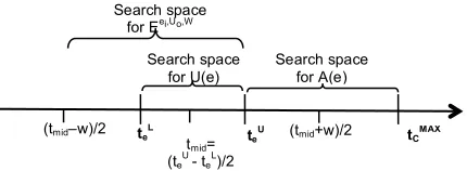
For consequent events e that cannot be unified with any event in the log, i.e., when U(e)=∅, the computation of mGN depends on the latest timestamp of the captor of e, t
cmax. If tcmax < teU, the occurrence of
an event matching e cannot be precluded. In such cases, mGN remains agnostic by assigning a zero basic
probability to Ge,Uo,W and ¬Ge,Uo,W. If t
cmax≥ teU,mGN assigns a zero basic probability to the genuineness of e
because there is no event matching it. However, since tcmax is determined by the time stamp of the latest event
received from captor c, its accuracy would also need to be assessed. This is because if the event with timestamp tcmax is not genuine, tcmax will not be correct. To address this possibility, mGN computes the basic
probability of the non genuineness of the event of interest (i.e., ¬Ge,Uo,W) as the combined basic probability of the genuineness of the events in the log that have occurred after teU (i.e., the basic probability assigned to the
disjunction ∨ei⊆A(e) E
ei,Uo,W). This is because if all the events in A(e) are confirmed by valid explanations, then
captor c’s time is more likely to have progressed beyond teU and, therefore, the absence of events matching e
[image:12.595.170.385.377.456.2]would be more certain. Fig. 4 presents the time ranges that underpin the formulation of sets U(e), A(e) and the proposition Eei,Uo,W.
Figure 4. Time ranges for U(e), A(e) and Eei,Uo,W
The functional form of the BPA mG and the belief function induced by it are derived by the following
theorem.
Theorem 1: Let U(e) and A(e) be non empty set of runtime events, Eei,Uo,W be a proposition denoting that
a concrete event ei in U(e) or A(e) has a valid explanation within the time range [tmid−w/2, tmid+w/2], and
¬Eei,Uo,W be a proposition denoting that e
i has no valid explanation within the time range [tmid−w/2,
tmid+w/2].
(a) The BPA mEX defined as mEX = m
1EX⊕ m2EX⊕ … ⊕ mnEX where miEX (i=1,…,n; n=|U(e)| or n=|A(e)|) are
the BPA functions defined in Definition 2 has the following form:
mG(x) =
ΠiεImi
EX(Eei,Uo,W)×Π jεI'mj
EX(
¬Eej,Uo,W)
if x= ∩iεIE
ei,Uo,W∩ jεI'¬E
ej,Uo,W
for all I, I' such that I
⊆ S & I' = S − I where S=U(e) or S=A(e)3
0 if x≠∩iεIE
ei,Uo,W∩ jεI'¬E
ej,Uo,W
(b) The beliefs to the propositions ∨ei∈U(e) E
ei,Uo,W, ∧ ei∈U(e) ¬E
ei,Uo,W and ∨ ei⊆A(e) E
ei,Uo,W produced by the belief
function induced by mG are computed by the following formulas:
BelG(∨ ei∈U(e) E
ei,Uo,W) = Σ
I⊆U(e) and I≠Ø(−1)
|I|+1{ Π i∈I mi
EX(Eei,Uo,W)}
BelG(∧ei∈U(e) ¬E
u,Uo,W) = Π ei∈U(e) mi
EX(
¬Eei,Uo,W)
3 For any two sets identified as I and I', I' denotes the complement set of I with respect to some common set S. Unless defined otherwise in a theorem or definition, I' denotes the complement set of I w.r.t the common frame discernment
θ defined in [38]. tmid=
(teU - teL)/2
(tmid–w)/2 teL teU (tmid+w)/2 tCMAX
Search space
for U(e) Search space for A(e) Search space
BelG(∨ ei⊆A(e) E
ei,Uo,W) =Σ
I⊆ A(e) and I≠Ø(−1)
|I|+1{ Πi∈I mi
EX(Eei,Uo,W)}
The proof of Theorem 1 is given in [38]. Based on it, the belief in event genuineness is computed as:
(i) if U(e)≠∅
BelG(P) =
ΣI⊆U(e) and I≠Ø(−1) |I|+1{
Πi∈I mi
EX(Eei,Uo,W)} if P=Ge,Uo,W
Πu∈U(e) mi EX(
¬Eei,Uo,W) if P=¬Ge,Uo,W
(ii) if U(e)=∅
BelG(P) =
0 if P= Ge,Uo,W or P= ¬Ge,Uo,W, and tcmax < teU
0 if P= Ge,Uo,W and t
cmax≥ teU
ΣI⊆A(e) and I≠Ø (−1) |I|+1{
Πi∈I mi
EX(Eei,Uo,W)} if P= ¬Ge,Uo,W and t
cmax≥ teU
BelG depends on the BPA m
iEX for computing the basic probability of the existence or not of a valid
explanation for a concrete event ei. The BPA function miEX is defined as follows.
Definition 2: The BPA function miEX for the existence of a valid explanation for a runtime event ei is defined
as:
(a) if EXP(ei)≠∅:
miEX(P) =
mVL(!Êj∈EXP(ei) VL(ei,Êj,Uo,W)) if P= E ei,Uo,W
mVL("
Êj∈EXP(ei) (¬VL(ei, Êj,Uo,W)) if P=¬E ei,Uo,W
(b) if EXP(ei) = ∅
miEX(P) =
α1 if P= Eei,Uo,W
1 −α1 if P= ¬Eei,Uo,W
where,
• EXP(ei)is the set of possible explanations generated by abduction for ei and Êj is an explanation in this
set,
• VL(ei,Êj,Uo,W) (¬VL(ei,Êj,Uo,W)) is a proposition denoting that Êj is (not) a valid explanation for ei given
the events in the log within the range [tmid–w/2, tmid+w/2] excluding those in Uo,
• α1 is a parameter taking values in [0,1] determining the default basic probability of event genuineness in
the case of events that have no explanation (α1 should be set to 0 if such events need to be considered as
non genuine events), and
• mVL is the BPA function resulting from the combination of the basic probability assignments miVL to the
propositions VL(ei,Êj,Uo,W) and ¬VL(ei,Êj,Uo,W) i.e., mVL = m1VL⊕ m2VL ⊕ … ⊕ mnVL where n=|EXP(ei)|.
The BPA functions miVL are defined in Definition 3. q
According to Definition 2, an event is considered to have an explanation if at least one of the alternative explanations found for it is valid (see disjunction ∨Êj∈EXP(ei) VL(ei,Êj,Uo,W)), and not to have an explanation if none of its alternative explanations is valid (see conjunction ∧Êj∈EXP(ei) (¬VL(ei, Êj,Uo,W)). The functional form of mVL is given by Theorem 2.
Theorem 2: Let eu be a runtime event, EXP(eu) be a non empty set of explanations of eu, and VL(eu,Ê,Uo,W)
and ¬VL(eu,Ê,Uo,W) be the propositions defined in Definition 2.
(a) The combined basic probability assignment mVL defined as mVL = m
1VL⊕ m2VL⊕ … ⊕ mnVL will be the
function:
mVL(x) = ΠiεImi
VL(VL(e
u,Êj,Uo,W))×ΠjεI'mj
VL(¬VL(e
u,Êj,Uo,W)) if x= ∩iεIVL(eu,Êj,Uo,W) ∩jεI'¬VL(eu, Êj,Uo,W)
0 if x≠∩iεI VL(eu,Êj,Uo,W) ∩jεI'¬VL(eu, Êj,Uo,W)
(b) The beliefs to the propositions ∨Êj∈EXP(eu) VL(eu,Êj,Uo,W) and ∧Êj∈EXP(eu)¬VL(eu, Êj,Uo,W) produced by the
belief function induced by mVL will be: BelVL(∨
Êj∈EXP(eu) VL(eu,Êj,Uo,W)) =ΣI⊆EXP(eu) & I≠Ø (−1)
|J|+1{ ΠÊj∈I mj
VL(VL(e
u,Êj,Uo,W))}
BelVL(∧
Êj∈EXP(eu)¬VL(eu,Êj,Uo,W)) = Π Êj∈EXP(eu) mj
VL(
where mjVL (j=1,…,|EXP(eu)|) are the basic probability assignment functions defined in Definition 3.
The proof of Theorem 3 is given in [38]. Based on this theorem, the belief in the existence or not of a valid explanation for a runtime event, if it is possible to identify at least one explanation through the abductive reasoning process described in Sect. IV, is computed as:
BelVL(P) = ΣJ
⊆EXP(ei) & J≠Ø (−1) |J|+1 {
Π Êj∈J mj VL(VL(e
i,Êj,Uo,W))} if P = Eei,Uo,W
Π Êj∈EXP(ei) mj VL(
¬VL(ei, Êj,Uo,W)) if P = ¬Eei,Uo,W
In cases when EXP(ei)=∅, BelVL(Eei,Uo,W) = α1 and BelVL(¬Eei,Uo,W) = 1 −α1. These formulas result from
(a5) and the definition of mVL.
D. Belief in explanation validity
The BPA to the validity of an explanation is defined as:
Definition 3: The BPA for the validity of an explanation Êj for a runtime event ei is defined as:
(a) if GN(ei, Êj Uo,W) ≠∅
mjVL(P) =
mCN(∨
ej∈CN(ei,Êj,Uo,W) G
ej,Uo,W) if P = VL(e
i,Êj,Uo,W)
mCN(∧
ej∈CN(ei, Êj,Uo,W) ¬G
ej, Uo,W) if P = ¬VL(e
i,Êj,Uo,W)
(b) if GN(ei, Êj,Uo,W) = ∅
mjVL(P) =
α2 if P = VL(ei,Êj,Uo,W)
1 −α2 if P = ¬VL(ei,Êj,Uo,W)
where,
• GN(ei,Êj,Uo,W)is the set of the consequent events that the explanation Êj has in the time range defined by
W excluding any events in Uo and ei or, formally, GN(ei,Êj,Uo,W)= {c | ({Êj, AS, L} |= c) and (c∉Uo) and
(c≠ei) and (tmid – w/2 ≤ tcL) and (tcU≤ tmid+w/2)} where , AS is the set of system assumptions and L is the
monitor’s event log.
• α2 is a parameter taking values in [0,1] that provides the default basic probability of the validity of an
explanation that has no consequences (α2 should be set to 0 if such explanations should be totally
disregarded for a given system).
• mCN is the belief function resulting from combining the BPAs to the genuineness of the consequences of individual explanations, i.e., mCN = m1GN⊕ m2GN ⊕ … ⊕ mnGN where n=|GN(ei,Ê,Uo,W)|. q
mVL computes the basic probability of the validity of an explanation Ê as the basic probability of at least
one of the consequences of Ê being a genuine event, and the basic probability of the non-validity of Ê as the basic probability of none of the consequences of Ê being a genuine event.
The functional form of mECN is given by the following theorem.
Theorem 3: Let Ê be a possible explanation for a runtime event eu, GN(eu,Ê,Uo,W) be the set of the
consequences that Ê has in the time range defined by W excluding events in Uo and eu, and Ge,Uo,W, ¬Ge,Uo,W
be the propositions denoting the genuineness and non genuineness of the events e GN(eu,Ê,Uo,W),
respectively.
(a) The combined basic probability assignment mCN defined as mCN = m
1GN⊕ m2GN⊕ … ⊕ mnGN will be the
function:
mCN(x) =
ΠiεImi
GN(Gei, Uo,W)×Π jεI'mj
GN(
¬Gej, Uo,W) if x=∩iεI G
ei,Uo,W∩ jεI'¬ G
ej,Uo,W
0 if x≠∩iεI G
ei,Uo,W∩ jεI'¬ G
ej Uo,W
where mjGN (j=1,…,|GN(eu,Ê,Uo,W)|) are the basic probability assignment functions defined in Definition 1.
(b) The beliefs to the propositions ∨ej∈CN(eu,Ê,Uo,W) G
ej,Uo,W and ∧
ej∈CN(eu,Ê,Uo,W)¬G
ej,Uo,W produced by the belief
function induced by mCN will be:
BelCN(∨
ej∈CN(eu,Ê,Uo,W) G
ej,Uo,W) = Σ
J⊆CN(eu,Ê,Uo,W) and J≠Ø (−1)
|J|+1{ Π ej∈J mj
GN(Gej,Uo,W)}
BelCN(∧
ej ∈ CN(eu,Ê,Uo,W) ¬ G
ej, Uo,W) = Π
ej ∈ CN(eu,Ê,Uo,W) mj
The proof of Theorem 4 is given in [38]. Based on this theorem, the belief in the validity of an individual explanation that has a non empty set of consequences is computed as:
BelCN(P) = ΣJ⊆CN(ei,Ê,Uo,W) & J≠Ø (−1) |J|+1{
Πej∈J mj
GN(Gej,Uo,W)} if P = VL(ei,Ê,Uo,W)
Πej ∈ CN(ei,Ê,Uo,W)mj GN(
¬Gej,Uo,W)
if P = ¬VL(ei,Ê,Uo,W)
In cases where an explanation Ê for an event has no consequences other than the event it was created to explain itself, the belief in the validity of the explanation is computed as:
BelCN(P) = α2 if P= VL(ei,Ê,Uo,W)
1 −α2 if P= ¬VL(ei,Ê,Uo,W)
The above form of BelCN is the direct consequence of axiom (a5) and the definition of mCN (Definition 3). It should also be noted that, as proved in [38], the functions mG, mVL and mEX satisfy the axioms of basic
probability assignments in the DS theory. In the following, we give an example of computing event genuineness beliefs using the above belief functions.
E. Example
Fig. 5 below shows a graph representing part of the diagnosis model of the LBACS system. The graph has been extracted from diagnostic assumptions for LBACS, expressed in EC-Assertion. The nodes and edges of the graph represent EC-Assertion formulas as indicated in the key of the figure.
Based on this model, the Explain algorithm of Fig. 3 would generate the following explanation for an event E:Happens(e(e1,s1,r1,login(u1,101,n1),c1),10050,R(10050) in the monitor’s log:
Ê: Happens(e(e2, …, InPremises(101,n1),c2),t2, R(9050,10050))
Ê would be generated by abduction from the assumption A1 in the graph of Fig. 5. From Ê, the following expected consequences would also be derived by deduction:
• C1:Happens(e(_x,…,signal(101),…),t1,R(6050,10050)) (C1 is derived by deduction from the assumption
corresponding to the edge InPremises à signal in Fig 5)
• C2:Happens(e(_x,…,login(_U,101,_NS),…),t1,R(8050,10050))
(C2 is derived by deduction from the assumption corresponding to the edge InPremises à login)
• C3:Happens(e(_y,…,accessTo(101),…),t2,R(9050,69050))
[image:15.595.62.432.475.692.2](C3 is derived by deduction from the assumption corresponding to the edge InPremises à accessTo)
Figure 5. Part of LBACS diagnosis model
TABLE II. EXPLANATION VALIDITY AND EVENT GENUINENESS BELIEFS
Event Log mVL(Ê) mG(E)
Happens(e(…,signal(101)…), 8050, R(8050,8050) α2 +α2 −α2×α2 = 0.36 0.36
Happens(e(…,signal(101)…), 8050, R(8050,8050);
Happens(e(…,accessTo(101)…), 9801, R(9801, 9801) αα2 2+ (×αα22 ) = 0.488 +α2 −α2×α2 ) −α2× (α2 +α2 −
0.488
Thus, depending on the log of events, the beliefs in the validity of Ê and the genuineness of E would be as shown in Table II (the computations in Table II assume that α2 = 0.2 and W = 100000 milliseconds).
with events in the log. The belief in the validity of Ê increases in the second case, as there are more events in the log confirming the consequences of Ê.
V. EVALUATION
A. Objectives and experimental set up
To evaluate our approach, we have performed a series of experiments aimed at investigating: (a) the accuracy of the event assessment process, (b) possible factors that may affect this accuracy, and (c) the time required for the execution of the assessment process.
The experimental evaluation was based on a simulation of the LBACS industrial case study. The use of simulation was necessary in order to be able to introduce attacks in the communication lines of the system and investigate their effect on the assessment process. The model of LBACS used in the simulation is shown in Fig. 6. This model covered all the components of LBACS and associated the communication lines between these components with adversaries able to intercept, and block or delay events transmitted over the lines.
[image:16.595.148.391.378.558.2]The simulation model was used to generate different event logs for analysis. Each event log was generated by producing random seed events triggering interactions between LBACS components and then using the model to produce further events based on the specification of the components of the model. A request for accessing an LBACS resource sent by a mobile device to the access control server, for example, was a seed event generated at a random time point and with event parameter values (e.g., device ID) that were randomly selected from pre-specified sets of values having an equal probability of selection. Upon the receipt of such a seed request, the access control server would request the location of the device from the location server. The latter server would then respond according to its specification and with a random delay. Furthermore, adversaries could intervene in interactions by dropping or delaying randomly selected events. Adversary03 in Fig. 6, for example, could delay the request to the access control server or drop it altogether thus stopping the event sequence. Following a random choice to delay an event, an adversary introduced a random delay to it.
Figure 6. LBACS simulation model
Based on this process, we generated three groups of simulated events (G1, G2, and G3) to represent different levels of adversary intervention. Adversary intervention levels, or “attack sizes”, were measured by the number of the events affected by adversaries in a simulation (i.e., the number of delayed or dropped events). The level of intervention was set to 10 percent for G1, 20 percent for G2 and 30 percent for G3. Each of G1, G2 and G3 consisted of five different events sets consisting of 5000 random events each. All the five sets in each group had the same level of adversary intervention. The generated event sets were subsequently fed into EVEREST to execute monitoring and event assessment. In this process, we used 18 diagnostic assumptions.
The accuracy and degree of completeness of the event genuineness assessment process was measured separately for genuine and fake events, using the following formulas:
Pf = |EventsBR ∩ Eventsf| / |EventsBR| (1)
Pg = |EventsBR ∩ Eventsg| / |EventsBR| (2)
Rf = |EventsBR ∩ Eventsf| / |Eventsf | (3)
In these formulas, EventsBR is the set of events for which the assessment process generated a genuineness
belief in the range BR, Eventsg and Eventsf are the sets of genuine events and fake events generated in a
simulation respectively, and |•| is the cardinality of a set.
The first two of the above formulas measure the precision (accuracy) of the assessment process. More specifically, (1) measures the ratio of events with a genuineness belief in the range BR that are fake, and (2) measures the ratio of events with a belief in the range BR that are genuine (note that Pg = 1–Pf). The next two
formulas (i.e., (3) and (4)) measure the recall (i.e., extent of completeness) of the assessment process. In particular, (3) measures the ratio of fake events whose belief was in the range BR and (4) measures the ratio of genuine events whose belief was in the range BR.
In addition to different types of events (i.e., fake and genuine) and different ranges of genuineness beliefs, the precision and recall of the assessment process was investigated with respect to different sizes of assessment windows (W), and different attack sizes (AS). In particular, we investigated accuracy for:
• Three different belief ranges, namely a low belief range set to [0, 0.3), a medium belief range set to [0.3, 0.7) and a high belief range set to [0.7, 1.0].
• Five different assessment windows (i.e., windows of 1.5, 2.5, 5, 7.5 and 10 seconds).
• Three different attack sizes (i.e., simulations where the events affected by adversaries accounted for 10%, 20% and 30% of the entire event log produced in the simulation).
The outcomes of this investigation are discussed below. B. Precision and recall of assessment
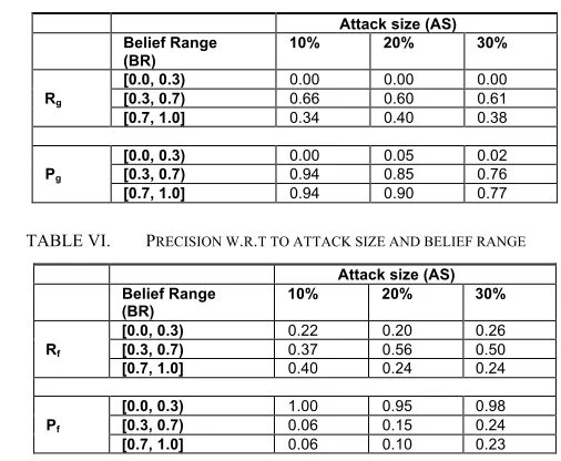
Tables III and IV show the precision and recall for genuine and fake events in the experiments, respectively. Precision and recall are shown for different belief ranges (BR) and sizes of the assessment window (W). The precision (Pg and Pf) and recall measures (Rg and Rg) shown in the tables have been
computed as averages across the five different sets of events that were generated in the simulations (i.e., a total of 25,000 simulated events), assuming an attack size of 20% (i.e., simulations where one in every five events was fake). The tables show also the average recall and precision measures, as computed across all five assessment windows, for the different belief ranges and genuine/fake events (see columns AVEW in the
tables). Graphs of the AVEW measures are also shown in Figures 7 and 8.
[image:17.595.157.408.575.713.2]Figure 7. Average precision/recall of genuine events
Figure 8. Average precision/recall of fake events
As Figure 7 shows, the average precision for genuine events (Pg) grows, as expected, from 0.47 at the
lower belief range to 0.88 at higher belief range. The same pattern was mirrored in the case of precision of
0.00 0.10 0.20 0.30 0.40 0.50 0.60 0.70 0.80 0.90 1.00
[0, 0.3) [0.3, 0.7) [0.7, 0.1] Belief Range
ave Rg ave Pg
0.00 0.10 0.20 0.30 0.40 0.50 0.60 0.70 0.80 0.90 1.00
[0, 0.3) [0.3, 0.7) [0.7, 0.1] Belief Range