Double-diffusive magnetic buoyancy instability in a quasi-two-dimensional Cartesian geometry

(1)

City, University of London Institutional Repository

Citation

:

Skinner, D. M. and Silvers, L. J. (2013). Double-diffusive magnetic buoyancy

instability in a quasi-two-dimensional Cartesian geometry. Monthly Notices of the Royal

Astronomical Society, 436(1), pp. 531-539. doi: 10.1093/mnras/stt1590

This is the published version of the paper.

This version of the publication may differ from the final published

version.

Permanent repository link:

http://openaccess.city.ac.uk/7394/

Link to published version

:

http://dx.doi.org/10.1093/mnras/stt1590

Copyright and reuse:

City Research Online aims to make research

outputs of City, University of London available to a wider audience.

Copyright and Moral Rights remain with the author(s) and/or copyright

holders. URLs from City Research Online may be freely distributed and

linked to.

City Research Online:

http://openaccess.city.ac.uk/

[email protected]

(2)

Advance Access publication 2013 September 26

Double-diffusive magnetic buoyancy instability in a

quasi-two-dimensional Cartesian geometry

D. M. Skinner

‹

and L. J. Silvers

‹

Centre for Mathematical Science, City University London, Northampton Square, London, EC1V 0HB, UK

Accepted 2013 August 21. Received 2013 August 21; in original form 2012 January 19

A B S T R A C T

Magnetic buoyancy, believed to occur in the solar tachocline, is both an important part of large-scale solar dynamo models and the picture of how sunspots are formed. Given that in the tachocline region the ratio of magnetic diffusivity to thermal diffusivity is small it is important, for both the dynamo and sunspot formation pictures, to understand magnetic buoyancy in this regime. Furthermore, the tachocline is a region of strong shear and such investigations must involve structures that become buoyant in the double-diffusive regime which are generated entirely from a shear flow. In a previous study, we have illustrated that shear-generated double-diffusive magnetic buoyancy instability is possible in the tachocline. However, this study was severely limited due to the computational requirements of running three-dimensional magne-tohydrodynamic simulations over diffusive time-scales. A more comprehensive investigation is required to fully understand the double-diffusive magnetic buoyancy instability and its de-pendency on a number of key parameters; such an investigation requires the consideration of a reduced model. Here we consider a quasi-two-dimensional model where all gradients in thexdirection are set to zero. We show how the instability is sensitive to changes in the thermal diffusivity and also show how different initial configurations of the forced shear flow affect the behaviour of the instability. Finally, we conclude that if the tachocline is thinner than currently stated then the double-diffusive magnetic buoyancy instability can more easily occur.

Key words: instabilities – MHD – Sun: interior – Sun: magnetic fields.

1 I N T R O D U C T I O N

The leading models of the large-scale solar dynamo posit that a toroidal magnetic field is generated from a poloidal field deep be-neath the surface of the Sun in the tachocline (see e.g. Silvers 2008; Charbonneau 2010, and references therein). The toroidal structures then become buoyant and rise towards the surface. The strongest of these magnetic filaments reach the surface to give rise to sunspot pairs. The weaker buoyant structures can be twisted in the solar convection zone, which is an important part of one large-scale dynamo model, namely, the interface model (Parker 1993). Therefore, given that the process of magnetic buoyancy is an integral part of both the sunspot formulation picture and mod-els of the large-scale solar dynamo, it is crucial that it is fully understood.

Magnetic buoyancy was first discussed by Parker (1955) and Jensen (1955) and since this time there has been considerable

_{E-mail: [email protected] (DMS); [email protected]} (LJS)

progress in understanding this process. Early research using lin-ear stability analysis derived stability criteria for ideal magnetohy-drodynamics and diffusive magnetohymagnetohy-drodynamics (see e.g. Parker 1966; Thomas & Nye 1975; Acheson 1979).

In the solar tachocline, while diffusivities are small they are non-negligible. Therefore, the most pertinent of these criteria to consider for structures in the tachocline is that derived by Acheson (1979):

−ga2

c2

d dzlnB >

η κN

2

(1)

whereBis the field strength,ηis the magnetic diffusivity,κis the thermal diffusivity,ais the Alfvén speed,cis the adiabatic sound speed andNis the Brunt–Väisälä frequency. In the tachocline,κη and it is this regime that we need to explore fully; this paper will focus on the magnetic buoyancy instability whenκ η. Given that the magnetic structures in the tachocline are generated by a shear flow it is important to numerically examine structures that are generated in this way as opposed to simply examining those that are unstable at the start of the simulation.

C

2013 The Authors

Published by Oxford University Press on behalf of the Royal Astronomical Society

at City University, London on March 26, 2015

http://mnras.oxfordjournals.org/

(3)

532 D. M. Skinner and L. J. Silvers

Seeking to understand the formation of shear generated magnetic buoyant structures is a complex issue because of the dynamic nature of the problem, which involves a number of different time-scales i.e. the advective time-scale associated with the generation of a layer of magnetic field, the time-scale associated with the instability and the diffusive time-scales. In this particular problem a shear flow will drag out a layer of magnetic field that is initially perpendicular to the direction of the large-scale flow. This will create gradients in the magnetic field, which are necessary to achieve for buoyancy as can be seen from criterion 1. However, the layer of magnetic field acts back on the flow, which reduces the shear flow’s effectiveness to generate gradients of magnetic field. Further, the background atmosphere will be altered and so the values of the components in criterion 1 for instability are constantly changing.

Research to date on the interaction between a shear flow and a magnetic field includes that of Tobias & Hughes (2004) who ex-amined the stability of an atmosphere where there is a flow aligned with the magnetic field and concluded that the shear has a sta-bilizing effect on the magnetic buoyancy instability. However, in the tachocline the shear is actually responsible for the generation of an unstable layer of magnetic field aligned with the shear flow where, in an idealized picture, none exists; this is a very different proposition. There have been a number of papers to examine shear generated magnetic buoyancy instabilities when the magnetic field is not initially in the direction of the shear flow (Cline, Brummell & Cattaneo 2003; Vasil & Brummell 2008; Silvers et al. 2009). Silvers et al. (2009) considered if the double-diffusive magnetic buoyancy instability could occur in the tachocline and were the first to numerically show that such an instability is plausible. This work follows earlier calculations and discussions (see Hughes & Weiss 1995; Schmitt & Rosner 1983, and references there in) re-garding a magnetic buoyancy instability that presents when the ratio of magnetic to thermal diffusivity becomes sufficiently small, i.e. a double-diffusive magnetic buoyancy instability.

While the work of Silvers et al. (2009) was pioneering in the area of numerical calculations of the double-diffusive instability, their investigation was inhibited by the computational costs associated with three-dimensional calculations using small diffusivities. As such, they were only able to conduct a very limited investigation into how the instability is affected by the parameters that appear in the formulation of the problem and, thus, a further investigation is warranted.

While the investigation of Silvers et al. (2009) was limited, it was sufficient to show that the initial stages of the instability are dominated by the rapid growth of two-dimensional modes. This finding is in agreement with works such as Newcomb (1961) that suggest that two-dimensional interchange modes will often present rather than three-dimensional bending modes. That said, modes that initially onset in a two-dimensional fashion can develop in a three-dimensional way though interactions with other motion, e.g. turbulence caused by descending convective plumes, and so are of interest when we are looking for long-term, three-dimensional buoyant structures and their evolution.

The work of Silvers et al. (2009) suggests that a useful avenue of investigation, to explore further how the various parameters affect the onset of the double-diffusive magnetic buoyancy instability, is through a reduced model, which will minimize the computational cost of exploring the parameter space. Such a model will be consid-ered in this paper where we wish to obtain a greater understanding of the onset parameters for double-diffusive magnetic buoyancy in-stabilities, which will be used in later calculations to investigate the three-dimensional evolution of these structures. The reduced model

that we use in this paper is such that gradients in thex-direction are neglected. This reduction permits a much fuller exploration of the parameter space and enables us to determine how certain parameters affect the onset of the instability and the growth rate.

2 N U M E R I C A L M O D E L

We consider a model similar to those presented in the three-dimensional work of Silvers et al. (2009) and Vasil & Brummell (2008) but we form a reduced model by neglecting gradients in one direction. In this work thexandycoordinates are the latitudinal and longitudinal directions, and thez-axis points vertically down and parallel to the constant gravitational acceleration. All lengths are scaled relative to the depth of the domain,d. The temperature,

T, is scaled relative toT∗, the temperature at the top of the domain. The density,ρ, is scaled relative toρ_∗the density at the top of the layer. The magnetic field,B, is scaled relative to the initial vertical magnetic field strength,Bz, 0. Time is scaled with the isothermal

sound crossing time at the top of the layer,τ∗=dρ1/2

∗ /P∗1/2. The

general governing equations are written in the form:

∂ρ

∂t + ∇.(ρv)=0, (2)

ρ

∂u

∂t +u.∇u

= −∇P+α(B.∇)B−α∇

B2

2

+σ Ck

∇2

u+1

3∇(∇.u)

+ρθ(m+1) ˆz+F (3)

∂T

∂t = −u.∇T−(γ−1)T∇.u+ Ckγ

ρ ∇

2_T

+Ck(γ−1)

ρ

αζ J2+σ 2S

2 ₍₄₎

∂B

∂t = ∇ ×(u×B)+ζ Ck∇

2

B, (5)

∇.B=0 (6)

where

Sij = ∂ui ∂xj

+∂uj ∂xi

−2

3

∂uk ∂xk

δij (7)

is the stress tensor.Ck=Kτ∗/ρ∗cpd2is the dimensionless thermal

diffusivity,α=B2

z,0/P∗μ0provides a measure of the field strength,

ζ =ηcpρ∗/Kis the inverse Roberts number,σ =μcpρ∗/Kis the

Prandtl number,θis the thermal stratification andmis the polytropic index.

Equation (3) has been augmented to include an extra body force,

G= −σ Ck∂2zU0(z)xˆ that, in the absence of magnetic effects or

instabilities, balances viscous diffusion and maintains a specified

U0(z), which is chosen to mimic the smooth radial shear transition

believed to occur in the tachocline. The shear profile is given by

U0(z)=Mtanh

1 z

z−1 2

[image:3.595.306.547.291.562.2]

. (8)

Fig. 1 shows the velocity shear profile plotted against depthzfor the initial parameter configuration whereM=0.05 andz=0.1.

(4)

[image:4.595.350.504.59.434.2]

Figure 1. Shear profile,U0(z), versus depth,z, for the case used for the

initial cases whereM=0.05 andz=0.1.

The above set of equations is further simplified by removing all gradients of quantities in thex-direction, i.e. we set

∂

∂xf(x, y, z, t)=0 (9)

for all quantities.

Boundary conditions for the velocity,v, and the magnetic field,

B, are ∂zu=∂zv=w=0 and Bx=By=∂zBz=0 at the top

and bottom of the domain,z = 0, 1. The boundary conditions for temperature areT(z= 1)= 1 and∂Tz(z=0)=θ. Periodic

boundary conditions are taken in both thexand theydirections. These simulations are conducted using resolutions up to 256×480. Initially we take a polytropic atmosphere with temperature T0=1+θzˆ and density ρ0=(1+θˆz)m. We also initially set

Bz=1,ux=U0(z),uy=uz=Bx=By=0. The system is forced

out of equilibrium state by a small initial random perturbation to the temperature field. The governing equations are solved using a mixed finite difference/pseudo-spectral scheme as discussed in, for example, Bushby & Houghton (2005).

In this investigation we will allow a number of parameters to vary but there are some parameters that will remain fixed for the entire paper. For all of the cases that we consider in our investigation we takeF=1.25×10−5_,_θ₌_{5 and}_m₌_1.6.

3 R E S U LT S

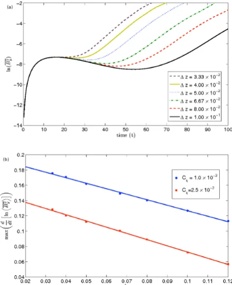
The double-diffusive magnetic buoyancy instability relies on the ratio between the magnetic and thermal diffusivities being small. Accordingly, the main focus of this paper is to see how the onset and growth rate of the instability, not its non-linear evolution, are affected by changing this ratio. Hence we will begin by examining the effect on the onset of the instability of varying the dimensionless thermal diffusivity,Ck. We note here that, for all results presented

in this paper the Richardson number is such that the shear flow is stable, i.e. there is no secondary instability that can influence the results.

In this investigation we choose principally to adjust the ratio of magnetic to thermal diffusivities by varying the thermal diffusiv-ity (via its dimensionless counterpartCk). As we varyCkwe also

adjust the Prandtl number,σ, and the inverse Roberts number,ζ, so as to maintainσCk =2.5×10−6andζCk=5.0×10−6thus

leaving the form of the induction equation unchanged and chang-ing the dynamics through the temperature equation. This method ensures that the magnetic Prandtl number is fixed, which aids

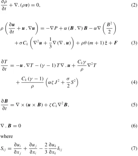
Figure 2. A comparison of the vertical component of velocity at compa-rable times for a slice of the three-dimensional case (top) and a quasi-two-dimensional run (middle). The bottom image shows density perturbation from the horizontal averaged value.

comparison with the work of Silvers et al. (2009). It is also possi-ble to vary the inverse Roberts number,ζ, effectively varying the magnetic diffusivity without scalings and so changing the dynamics directly through the induction equation (5). This would give rise to a variable magnetic Prandtl number. For brevity we limit the full dis-cussion here to considering the case whereCKis varied but we will

make comment at the end about the effect of varying the magnetic diffusivity.

Before we commence our investigation, we begin by illus-trating that this reduced model captures the essential dynamics of fully three-dimensional calculations, such as those shown in Silvers (2008). Fig. 2 shows a comparative slice from a fully three-dimensional and a quasi-two-three-dimensional calculation after the onset of the instability for the same set of parameters (case A1 in Table 1). Both simulations were started from the equilibrium solution with the same, small amplitude perturbation, to the temperature value at each point.1 _{The resolution for the three-dimensional case is}

1_{Note the image shown in Silvers et al. (2009) was started and evolved}

at early times in a slightly different way and found a slightly different lengthscale for the instability.

[image:4.595.47.284.59.214.2]

(5)

[image:5.595.306.547.57.204.2]

534 D. M. Skinner and L. J. Silvers

Table 1. Critical values for instability for different values ofz.

z Critical value 5.0×10−2 _6.355_×₁₀−4

6.67×10−2 _7.692_×₁₀−4

[image:5.595.57.273.77.297.2]

1.0×10−1 _1.137_×₁₀−3

Figure 3. A scatter plot formed from the data at each point for the vertical velocity and the density perturbation from the horizontal average.

Figure 4. A volume rendering of vertical velocity taken at the same in-stance as the slices shown in Fig. 2 for case A1 and shows the initial two-dimensional nature of the instability.

256×256×480 and the resolution for the quasi-two-dimensional case is 256×480. Fig. 2 shows that, although the two slices are not exactly identical for the different calculations, the instability onsets with the same lengthscale. Fig. 2 also shows the density deviation from the layer average value and shows that the rising structures are less dense, as you would expect with structures arising from a buoyancy instability. The formal correlation between vertical ve-locity and the density deviation from the layer average at the time of the images shown in Fig. 2 is given in Fig. 3. This scatter plot shows a good agreement between the two quantities. Further, Fig. 4 shows that, as discussed in Silvers (2008), the instability onsets in a two-dimensional form. Thus, our reduced model captures the essential features of the fully three-dimensional calculation.

We commence our discussion of our findings by varying the ratio of magnetic to thermal diffusivities via varyingCk. The Richardson

[image:5.595.308.545.256.395.2]

numbers, together with all of the exact parameter combinations for these cases, are given in a table in the Appendix. The background magnetic field is initially uniform in the z-direction. During the initial stages of the simulation there is a build up of thexcomponent of the magnetic field as the zcomponent is stretched out by the shear flow. During this period, theycomponent of the magnetic field undergoes small fluctuations due to the initial perturbation of

Figure 5. lnB2

y versus time for different values of the dimensionless

[image:5.595.68.259.337.446.2]

ther-mal diffusivity,Ck. The data points correspond to cases A1–A10 shown in Table A1.

Figure 6. The maximum value of d(lnB2

y)/dt versus the dimensionless

thermal diffusivityCkfor different values of the shear width,z. The data points correspond to cases A1–A10, H1–H11 and I1–I12 in Tables A1 and A3.

the system, before settling back down towards zero, which is shown in Fig. 5. When the instability occurs large disturbances inBybegin

to appear and Fig. 5 shows that the rate of growth ofB2

yis noticeably

reduced asCkdecreased from the value set in our reference case,

A1, which is 1.0×10−2_.

In this investigation we are principally interested in determining if an instability occurs so we focus our attention to the parts of the simulation long before boundary effects etc. are seen. For each of the cases we determine the maximum value of d(lnB2

y)/dtand the

time that it occurs after the initial transient phase. Fig. 6 shows the maximum value of d(lnB2

y)/dtfor cases A1–A10 where the only

parameter that is varied isCk. It shows that the maximum value of

d(lnB2

y)/dttends to zero as we reduceCkwhenz=1.0×10−1

(the figure also shows otherzcases that will be discussed later). A negative value for d(lnB2

y)/dtindicates thatBy2is tending to zero,

thus implying that there is no magnetic buoyancy instability. As the maximum value of d(lnB2

y)/dtapproaches zero it becomes difficult

to accurately determine the maximum value due to numerical issues and so a spline interpolant is used to extrapolate from the values plotted to determine the value ofCkfor which the instability no

longer occurs, which is approximately 1.2×10−3_{. Fig. 6 shows}

that by plottingB2

y for case A10, whereCk=1.25×10−3, there

is a small increase ofB2

ywith time. However, for case A11, where Ck=1.0×10−3, there is a constant decrease. Thus we conclude

that the instability is dependant onCkbeing sufficiently large.

(6)

There is a criterion proposed to determine when the double-diffusive magnetic buoyancy instability might be present. Vasil & Brummell (2009) derived a new form of the criterion for magnetic buoyancy instability when a background state is constantly evolv-ing. This is a more realistic model than that originally envisioned by Acheson who did not try to account for the back-reaction effect of the magnetic field on to a shear flow. The criterion proposed by Vasil & Brummell (2009) is expressed in a form where the magnetic field does not explicitly appear but where, instead, the shear flow that generates a layer of unstable magnetic field appears though the Richardson number and the width of the shear region itself. The analytic criterion derived by Vasil & Brummell (2009) for magnetic buoyancy in an isothermal process is

z 4γ Hp

1+ z 2Hρ

ζ Ri

(γ−1)ζ+1. (10)

This expression shows that the threshold for instability will be af-fected not only by the ratio of magnetic to thermal diffusivities but also by the parameters associated with the shear forcing. While the double-diffusive magnetic buoyancy instabilities that we are inves-tigating are not really isothermal they are closer to isothermal than adiabatic. We, therefore, will consider criteria (10) as a reference and now turn to examine how well this criterion is satisfied.

Fig. 7 shows, for the cases we are considering here, both the left-hand and right-left-hand sides of inequality (10) for different values of

Ckand shows that the inequality is satisfied for the cases that lead

to instability. The region where the inequality is satisfied covers a larger area for the higher values ofCk where we have already

observed that the strength of the instability is at its greatest. While the criterion appears useful it should be noted that the inequality does, also, remain satisfied for small regions for some values ofCk

that do not lead to instability (anything less thanCk≈1.2×10−3

is stable.). This is attributed to the fact that the stability criterion is analytically derived under assumptions for magnetic buoyancy instability in the isothermal limit so we would not expect complete agreement with the results. However, our findings show that this criterion is useful as a guide even when not fully in the isothermal regime.

Criterion (10) suggests that the regime where the instability will occur should also depend on a number of other parameters which

Figure 7. The solid black line that sweeps from the top left to the bottom right plots the left-hand side of inequality (10) versus depth (on the horizontal axis). The other three lines plot the right hand side forCk=1.0×10−2

(pale green dashed line),Ck=2.5×10−3_{(dark green dash–dotted line)}

andCk=1.25×10−3_{(red solid line), all versus depth. The regions where}

these lines are below the black line are where the inequality is satisfied for instability.

include both the width of the shear flow and the magnitude of the shear flow. From observations, we only have an upper bound on the width of the tachocline and so it is important to understand how the width of the shear flow affects our findings. We adjust the width of the shear flow by varyingzin equation (8).

Fig. 6, that was discussed earlier for the case when z=1.0×10−1_{, also shows the maximum value of d(ln}_B2

y)/dt

plotted against the dimensionless thermal diffusivity,Ck, when the

shear width is z = 6.67 ×10−2_{, which corresponds to cases}

H1–H12, and whenz=5.0×10−2_{, which corresponds to cases}

I1–I12. The spline interpolant curves through the data points are all similar in shape and Table 1 shows the critical values for each case. The critical value forCk decreases as we reducez; this implies

that the greater the width of the region of shear is in the tachocline, the smaller the ratio of magnetic to thermal diffusivities must be to obtain magnetic buoyancy. Also, the maximum value of d(lnB2

y)/dt

for any givenCkis greater as we reducez; this implies that the

width of the shear region affects the strength of the instability. Given that at this present time we only have an upper bound on the width of the tachocline the results in this section suggest that if the tachocline is narrower then the ratio of magnetic to thermal diffusivities would need to be less extreme for this instability to occur. Further, a nar-rower tachocline would give rise to a more vigorous formation of strong structures.

Fig. 8(a) shows lnB2

yplotted against time for different values of

[image:6.595.310.547.368.659.2]

z(corresponding to cases A1, H1, I1, K1, L1 and M1) and shows that, when all other parameters are fixed, the instability onsets earlier

Figure 8. (a) lnB2

y versus time for different values of the shear width,

z. The data points correspond to cases A1, H1, I1, K1, L1, M1. (b) The maximum value of d(lnB2

y)/dtversus the shear width,z. The data points

for whenCk=1.0×10−2_{correspond to cases A1, H1, I1, K1, L1 and M1}

and the data points for whenCk=2.5×10−3correspond to cases A6, H6, I6, K2, L2 and M2 in Tables A1 and A3.

[image:6.595.48.285.512.658.2]

(7)

[image:7.595.307.545.56.203.2]

536 D. M. Skinner and L. J. Silvers

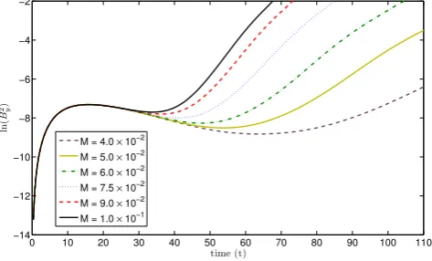
Figure 9. lnB2

yversus time for different values of the shear magnitude,M.

The data points correspond to cases A1, B1, C1, D1, E1 and F1 in Tables A1 and A2.

aszis decreased. This is because the depth of the vertical region in whichBxis stretched out is determined by the shear width and,

therefore, becomes narrower aszis reduced. The narrowing of this shear region causes the build up ofBxto happen faster, which

is a result of the fact thatBxis dependent on the velocity gradient

∂zU0(z) (Vasil & Brummell 2009). The faster build up and narrower

shear region cause the gradients inBxto reach the critical value for

instability earlier and, therefore, the instability to occur sooner. We also note that the narrowing of the shear region also causes the instability to occur closer to the centre of the domain,z=0.5.

The maximum value of d(lnB2

y)/dt plotted against the shear

width forCk =2.5×10−3(cases A6, H6, I6, K2, L2, M2) and

Ck = 1.0×10−2 (cases A1, H1, I1, K1, L1, M1) is shown in

Fig. 8(b). This plot shows a linear relationship between the maxi-mum growth rate of the instability and the width of the shear region. Therefore, this plot suggests that further decreasing the width of the shear flow region would give rise to a stronger instability but far greater resolution in z would be required to investigate smaller values ofzthan are presented here.

In addition to considering how varying the width of the shear flow affects the instability it is also interesting to also examine how the strength of the shear flow, governed by our parameterM, affects the results. This will allow us to comment on what may occur in other stars with a similar internal structure to the Sun but where the magnitude of the shear flow is different.

Cases A1, B1, C1, D1, E1 and F1 only differ in the shear mag-nitude valueM. Fig. 9 shows that there is a non-linear relationship betweenMand the maximum value of d(lnB2

y)/dtthat is obtained

for each of these cases. In Fig. 10, the maximum value of d(lnB2

y)/dt

is plotted againstCkfor different values ofM. In this figure two

dif-ferentMvalues,M=7.5×10−2_and_M₌_1.0_×₁₀−1_{, are compared}

with the original case whereM=5.0×10−2_{and shows that the}

critical value ofCKfor the instability to occur becomes smaller as

Mis increased.

At the start of this section we commented on the fact that we wanted to consider the effect that varying the ratio of magnetic to thermal diffusivities has on the magnetic buoyancy instability and that there were two possible ways to change this ratio. First, we chose to maintain the magnetic diffusivity and vary the thermal dif-fusivity and so change the dynamics via the temperature equation and not the induction equation that evolves the magnetic field; the evolution of which is of greatest interest in this work. However, we could have chosen to vary the ratio via changing the magnetic

y)/dt versus the dimensionless

[image:7.595.45.282.60.203.2]

thermal diffusivity,Ck, for different values of the shear magnitude,M. The data points correspond to cases A1–A10, B1–B14 and C1–C15 in Tables A1 and A2.

y)/dtversusζfor different values

of the shear width,z. The data points correspond to cases A1–A10, H1– H12 and I1–I12 from Tables A1 and A3.

diffusivity and so directly alter the induction equation. Given that one approach directly affects the evolution of the magnetic field and the other indirectly, through the temperature equation, these two approaches are not equivalent. Therefore, we will now briefly turn our attention to a discussion of the findings of how our results change, whenzis varied, if we had selected the alternative ap-proach whereCkis fixed and the non-dimensional parameter in our

equations is changed through varying,η.

Fig. 11 shows how the maximum value of d(lnB2

y)/dt varies

as ζ is varied for different values of the shear width, z. The data in this figure corresponds to cases A1–A10 in Table 1 where z=1.0×10−1_{, H1–H12 in Table A3 where}_z₌_6.67_×₁₀−2

and I1–I12 in Table A3 where z = 5.0 ×10−2_{. Once again,}

we find that Fig. 11 shows that, for each value ofz, there is a critical point that bounds the regime where the instability occurs. The critical point determines the greatest value ofζ for which the instability occurs. As we varyzwe find critical values as fol-lows: for z = 5.0 ×10−2 _{the critical value is approximately}

3.599×10−2_{, for}_z₌_6.67_×₁₀−2_{the critical value is}

approxi-mately 2.89×10−2_{, and for}_z₌_1.0_×₁₀−1_{the critical value is}

approximately 1.953×10−2_{. Thus, for fixed}_C

kincreasing the shear

width increases the value below which instability occurs. We note though that for any given value ofζfor this fixedCkinvestigation,

decreasing the width of the shear region makes this instability more likely to occur. Thus, as was stated earlier for the variableCkcase, if

[image:7.595.307.544.263.401.2]

(8)

the tachocline is narrower than the ratio of magnetic to thermal in-stabilities would need to be less extreme for this instability to occur. Further, a narrower tachocline would give rise to a more vigorous formation of strong structures.

4 C O N C L U S I O N S

To obtain a full understanding of how the large-scale solar dynamo operates it is vital that we understand what conditions lead to buoy-ant structures being formed in the tachocline. There are still some unknowns when we are considering the tachocline region and fur-ther it is currently impossible to conduct full numerical simulations at the extreme values of some of the parameters. Therefore, it is im-portant that we seek to explore how varying different quantities in the problem affect the formation of structures and to obtain scaling laws where possible.

In this paper we have presented the results from an investigation into the double-diffusive magnetic buoyancy instability. We chose to consider a quasi-two-dimensional model to enable a full exploration of how varying the key parameters associated with the problem affected the onset and initial phase of the instability. Our investi-gation primarily explored how varying the dimensionless thermal diffusivity, which varied the inverse Roberts number, affected the onset of the instability. The critical value for the thermal diffusivity translates into an upper bound on the ratio of magnetic to thermal diffusivity.

While in the tachocline we know that the ratio of magnetic to thermal diffusivities will be small, though exactly how small is not fully known, we still only have an upper bound at the present time on the thickness of the tachocline. Therefore, part of our research in this paper examined how the critical threshold value of the ther-mal diffusivity changed as we varied the width of the shear flow. We showed that varying the width of the shear flow by itself gives rise to a lower critical thermal diffusivity value for the onset of the instability. We have shown that the value ofCkfor the instability to

exist is dependent on the width of the shear region and the magni-tude of the shear flow. Further, we have shown that the maximum value of the growth rate varies linearly with the width of the shear flow.

One of the principal motivations for undertaking this reduced study was to ascertain information that would inform later three-dimensional investigations to examine the evolution of structures formed by the double-diffusive instability. Our work has provided crucial information for such investigations as it has determined what part of the parameter space is unstable whenσCk=2.5×10−6and

ζCk=5.0×10−6. We have shown that forM=5.00×10−2the

system is unstable for z < 0.1 provided Ck > 1.25× 10−3.

Further, we have shown that for fixed z, increasing M leads to a more unstable system. These results provide a firm foun-dation on which later three-dimensional investigations can be undertaken.

In the latter part of this paper, we discussed the effect of taking the alternative approach to this problem by varying the ratio of magnetic diffusivity to thermal diffusivity by altering the magnetic diffusivity. We showed that while the critical value ofζ, which translates into an effective value of the magnetic diffusivity, increases as you decrease

the shear flow, for any given magnetic diffusivity (with all other parameters fixed) as you decrease the width of the shear flow it becomes increasingly likely that instability will occur.

This work has shown, as anticipated from earlier work, that there is a critical value for which the double-diffusive instability will occur. While the diffusive parameters that can be considered nu-merically are much larger than in the solar tachocline there will be a critical value of thermal diffusivity, at constant magnetic Prandtl number, for this instability to occur. Further, this work in vary-ing the width of the shear flow region has shown that, if the solar tachocline is thinner than currently predicted, then double-diffusive magnetic buoyancy instability becomes more plausible as the ratio of magnetic to thermal diffusivities does not need to be so small for instability to occur. Once the width of the so-lar tachocline has been precisely determined, and the value of the transport coefficients obtained, we will be able to discuss fully if a double-diffusive magnetic buoyancy instability can exist in the tachocline.

Also, this work has provided a little insight into the magnetic buoyancy mechanism in other stars where the shear strength and width may be very different from the Sun. We have shown that as the strength of the shear is decreased, there appears to be a value below which the instability does not occur. This can be ex-plained by the fact that sufficiently large gradients in the magnetic field are not being created to give rise to an instability and dif-fusive spreading of the generated magnetic field dominates. This would suggest that the presence of a tachocline in other stars would not be sufficient for magnetic buoyancy and, by current thinking for the solar cases, insufficient for a large-scale dynamo in other stars.

AC K N OW L E D G E M E N T S

DMS would like to thank City University London for the award of a PhD studentship. We would like to thank the referee for very helpful suggestions and comments on the paper.

R E F E R E N C E S

Acheson D. J., 1979, Sol. Phys., 62, 23

Bushby P. J., Houghton S. M., 2005, MNRAS, 362, 313 Charbonneau P., 2010, Living Rev. Solar Phys. 7, 3

Cline K. S., Brummell N. H., Cattaneo F., 2003, ApJ, 599, 1449 Hughes D. W., Weiss N. 0., 1995, J. Fluid Mech., 301, 383 Jensen E., 1955, Ann. Astrophys., 18, 127

Newcomb W. A., 1961, Phys. Fluids, 4, 391 Parker E. N., 1955, ApJ, 121, 491 Parker E. N., 1966, ApJ, 145, 811 Parker E. N., 1993, ApJ, 408, 707

Schmitt J. H. M. M., Rosner R., 1983, ApJ, 265, 901 Silvers L. J., 2008, RSPTA, 366, 4453

Silvers L. J., Vasil G. M., Brummell N. H., Proctor M. R. E., 2009, ApJ, 702, L14

Thomas J. H., Nye A. H., 1975, Phys. Fluids, 18, 490 Tobias S. M., Hughes D. W., 2004, ApJ, 603, 785 Vasil G. M., Brummell N. H., 2008, ApJ, 686, 709 Vasil G. M., Brummell N. H., 2009, ApJ, 690, 783

(9)

538 D. M. Skinner and L. J. Silvers

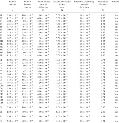
[image:9.595.84.510.105.270.2]

A P P E N D I X A

Table A1. The parameter values for the cases discussed when varyingCkonly.

Prandtl Inverse Dimensionless Maximum velocity Parameter controlling Richardson Instability number Roberts thermal for the the width number

number diffusivity shear of the shear

σ ζ Ck M z Ri

A1 2.50×10−4 _5.00_×₁₀−4 _1.00_×₁₀−2 _5.00_×₁₀−2 _1.00_×₁₀−1 _2.96 _Yes

A2 4.17×10−4 8.33×10−4 6.00×10−3 5.00×10−2 1.00×10−1 2.96 Yes A3 5.00×10−4 1.00×10−3 5.00×10−3 5.00×10−2 1.00×10−1 2.96 Yes A4 6.25×10−4 1.25×10−3 4.00×10−3 5.00×10−2 1.00×10−1 2.96 Yes A5 8.33×10−4 1.67×10−3 3.00×10−3 5.00×10−2 1.00×10−1 2.96 Yes A6 1.00×10−3 2.00×10−3 2.50×10−3 5.00×10−2 1.00×10−1 2.96 Yes A7 1.25×10−3 _2.50_×₁₀−3 _2.00_×₁₀−3 _5.00_×₁₀−2 _1.00_×₁₀−1 _2.96 _Yes

A8 1.43×10−3 _2.86_×₁₀−3 _1.75_×₁₀−3 _5.00_×₁₀−2 _1.00_×₁₀−1 _2.96 _Yes

A9 1.67×10−3 _3.33_×₁₀−3 _1.50_×₁₀−3 _5.00_×₁₀−2 _1.00_×₁₀−1 _2.96 _Yes

A10 2.00×10−3 _4.00_×₁₀−3 _1.25_×₁₀−3 _5.00_×₁₀−2 _1.00_×₁₀−1 _2.96 _Yes

A11 2.50×10−3 _5.00_×₁₀−3 _1.00_×₁₀−3 _5.00_×₁₀−2 _1.00_×₁₀−1 _2.96 _No Table A2. The parameter values for the additional cases needed whenMis varied.

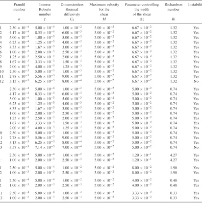
Prandtl Inverse Dimensionless Maximum velocity Parameter Controlling Richardson Instability number Roberts thermal for the the width Number

number diffusivity Shear of the shear

σ ζ Ck M z Ri

B1 2.50×10−4 _5.00_×₁₀−4 _1.00_×₁₀−2 _7.50_×₁₀−2 _1.00_×₁₀−1 _1.32 _Yes

B2 4.17×10−4 _8.33_×₁₀−4 _6.00_×₁₀−3 _7.50_×₁₀−2 _1.00_×₁₀−1 _1.32 _Yes

B3 5.00×10−4 _1.00_×₁₀−3 _5.00_×₁₀−3 _7.50_×₁₀−2 _1.00_×₁₀−1 _1.32 _Yes

B4 6.25×10−4 _1.25_×₁₀−3 _4.00_×₁₀−3 _7.50_×₁₀−2 _1.00_×₁₀−1 _1.32 _Yes

B5 8.33×10−4 _1.67_×₁₀−3 _3.00_×₁₀−3 _7.50_×₁₀−2 _1.00_×₁₀−1 _1.32 _Yes

B6 1.00×10−3 _2.00_×₁₀−3 _2.50_×₁₀−3 _7.50_×₁₀−2 _1.00_×₁₀−1 _1.32 _Yes

B7 1.25×10−3 _2.50_×₁₀−3 _2.00_×₁₀−3 _7.50_×₁₀−2 _1.00_×₁₀−1 _1.32 _Yes

B8 1.43×10−3 2.86×10−3 1.75×10−3 7.50×10−2 1.00×10−1 1.32 Yes B9 1.67×10−3 3.33×10−3 1.50×10−3 7.50×10−2 1.00×10−1 1.32 Yes B10 2.00×10−3 4.00×10−3 1.25×10−3 7.50×10−2 1.00×10−1 1.32 Yes B11 2.50×10−3 5.00×10−3 1.00×10−3 7.50×10−2 1.00×10−1 1.32 Yes B12 3.13×10−3 _6.25_×₁₀−3 _8.00_×₁₀−4 _7.50_×₁₀−2 _1.00_×₁₀−1 _1.32 _Yes

B13 4.17×10−3 _8.33_×₁₀−3 _6.00_×₁₀−4 _7.50_×₁₀−2 _1.00_×₁₀−1 _1.32 _Yes

B14 5.00×10−3 _1.00_×₁₀−2 _5.00_×₁₀−4 _7.50_×₁₀−2 _1.00_×₁₀−1 _1.32 _Yes

B15 6.25×10−3 _1.25_×₁₀−2 _4.00_×₁₀−4 _7.50_×₁₀−2 _1.00_×₁₀−1 _1.32 _No

C1 2.50×10−4 _5.00_×₁₀−4 _1.00_×₁₀−2 _1.00_×₁₀−1 _1.00_×₁₀−1 _0.74 _Yes

C2 4.17×10−4 _8.33_×₁₀−4 _6.00_×₁₀−3 _1.00_×₁₀−1 _1.00_×₁₀−1 _0.74 _Yes

C3 5.00×10−4 _1.00_×₁₀−3 _5.00_×₁₀−3 _1.00_×₁₀−1 _1.00_×₁₀−1 _0.74 _Yes

C4 6.25×10−4 _1.25_×₁₀−3 _4.00_×₁₀−3 _1.00_×₁₀−1 _1.00_×₁₀−1 _0.74 _Yes

C5 8.33×10−4 _1.67_×₁₀−3 _3.00_×₁₀−3 _1.00_×₁₀−1 _1.00_×₁₀−1 _0.74 _Yes

C6 1.00×10−3 _2.00_×₁₀−3 _2.50_×₁₀−3 _1.00_×₁₀−1 _1.00_×₁₀−1 _0.74 _Yes

C7 1.25×10−3 _2.50_×₁₀−3 _2.00_×₁₀−3 _1.00_×₁₀−1 _1.00_×₁₀−1 _0.74 _Yes

C8 1.43×10−3 _2.86_×₁₀−3 _1.75_×₁₀−3 _1.00_×₁₀−1 _1.00_×₁₀−1 _0.74 _Yes

C9 1.67×10−3 _3.33_×₁₀−3 _1.50_×₁₀−3 _1.00_×₁₀−1 _1.00_×₁₀−1 _0.74 _Yes

C10 2.00×10−3 4.00×10−3 1.25×10−3 1.00×10−1 1.00×10−1 0.74 Yes C11 2.50×10−3 5.00×10−3 1.00×10−3 1.00×10−1 1.00×10−1 0.74 Yes C12 3.13×10−3 6.25×10−3 8.00×10−4 1.00×10−1 1.00×10−1 0.74 Yes C13 4.17×10−3 8.33×10−3 6.00×10−4 1.00×10−1 1.00×10−1 0.74 Yes C14 5.00×10−3 _1.00_×₁₀−2 _5.00_×₁₀−4 _1.00_×₁₀−1 _1.00_×₁₀−1 _0.74 _Yes

C15 6.25×10−3 _1.25_×₁₀−2 _4.00_×₁₀−4 _1.00_×₁₀−1 _1.00_×₁₀−1 _0.74 _Yes

C16 8.33×10−3 _1.67_×₁₀−2 _3.00_×₁₀−4 _1.00_×₁₀−1 _1.00_×₁₀−1 _0.74 _No

D1 2.50×10−4 _5.00_×₁₀−4 _1.00_×₁₀−2 _9.00_×₁₀−2 _1.00_×₁₀−1 _0.92 _Yes

E1 2.50×10−4 _5.00_×₁₀−4 _1.00_×₁₀−2 _6.00_×₁₀−2 _1.00_×₁₀−1 _2.06 _Yes

F1 2.50×10−4 _5.00_×₁₀−4 _1.00_×₁₀−2 _4.00_×₁₀−2 _1.00_×₁₀−1 _4.63 _Yes

G1 2.50×10−4 _5.00_×₁₀−4 _1.00_×₁₀−2 _3.00_×₁₀−2 _1.00_×₁₀−1 _8.24 _Yes

[image:9.595.84.501.301.730.2]

(10)

[image:10.595.92.505.72.488.2]

Table A3. The parameter values for the additional cases required whenzis varied.

Prandtl Inverse Dimensionless Maximum velocity Parameter controlling Richardson Instability number Roberts thermal for the the width number

number diffusivity shear of the shear

σ ζ Ck M z Ri

H1 2.50×10−4 _5.00_×₁₀−4 _1.00_×₁₀−2 _5.00_×₁₀−2 _6.67_×₁₀−2 _1.32 _Yes

H2 4.17×10−4 8.33×10−4 6.00×10−3 5.00×10−2 6.67×10−2 1.32 Yes H3 5.00×10−4 1.00×10−3 5.00×10−3 5.00×10−2 6.67×10−2 1.32 Yes H4 6.25×10−4 1.25×10−3 4.00×10−3 5.00×10−2 6.67×10−2 1.32 Yes H5 8.33×10−4 1.67×10−3 3.00×10−3 5.00×10−2 6.67×10−2 1.32 Yes H6 1.00×10−3 2.00×10−3 2.50×10−3 5.00×10−2 6.67×10−2 1.32 Yes H7 1.25×10−3 _2.50_×₁₀−3 _2.00_×₁₀−3 _5.00_×₁₀−2 _6.67_×₁₀−2 _1.32 _Yes

H8 1.67×10−3 _3.33_×₁₀−3 _1.50_×₁₀−3 _5.00_×₁₀−2 _6.67_×₁₀−2 _1.32 _Yes

H9 2.00×10−3 _4.00_×₁₀−3 _1.25_×₁₀−3 _5.00_×₁₀−2 _6.67_×₁₀−2 _1.32 _Yes

H10 2.50×10−3 _5.00_×₁₀−3 _1.00_×₁₀−3 _5.00_×₁₀−2 _6.67_×₁₀−2 _1.32 _Yes

H11 2.78×10−3 _5.56_×₁₀−3 _9.00_×₁₀−4 _5.00_×₁₀−2 _6.67_×₁₀−2 _1.32 _Yes

H12 3.13×10−3 _6.25_×₁₀−3 _8.00_×₁₀−4 _5.00_×₁₀−2 _6.67_×₁₀−2 _1.32 _No

I1 2.50×10−4 _5.00_×₁₀−4 _1.00_×₁₀−2 _5.00_×₁₀−2 _5.00_×₁₀−2 _0.74 _Yes

I2 4.17×10−4 _8.33_×₁₀−4 _6.00_×₁₀−3 _5.00_×₁₀−2 _5.00_×₁₀−2 _0.74 _Yes

I3 5.00×10−4 _1.00_×₁₀−3 _5.00_×₁₀−3 _5.00_×₁₀−2 _5.00_×₁₀−2 _0.74 _Yes

I4 6.25×10−4 _1.25_×₁₀−3 _4.00_×₁₀−3 _5.00_×₁₀−2 _5.00_×₁₀−2 _0.74 _Yes

I5 8.33×10−4 _1.67_×₁₀−3 _3.00_×₁₀−3 _5.00_×₁₀−2 _5.00_×₁₀−2 _0.74 _Yes

I6 1.00×10−3 _2.00_×₁₀−3 _2.50_×₁₀−3 _5.00_×₁₀−2 _5.00_×₁₀−2 _0.74 _Yes

I7 1.25×10−3 _2.50_×₁₀−3 _2.00_×₁₀−3 _5.00_×₁₀−2 _5.00_×₁₀−2 _0.74 _Yes

I8 1.67×10−3 3.33×10−3 1.50×10−3 5.00×10−2 5.00×10−2 0.74 Yes I9 2.00×10−3 4.00×10−3 1.25×10−3 5.00×10−2 5.00×10−2 0.74 Yes I10 2.50×10−3 5.00×10−3 1.00×10−3 5.00×10−2 5.00×10−2 0.74 Yes I11 2.78×10−3 5.56×10−3 9.00×10−4 5.00×10−2 5.00×10−2 0.74 Yes I12 3.13×10−3 _6.25_×₁₀−3 _8.00_×₁₀−4 _5.00_×₁₀−2 _5.00_×₁₀−2 _0.74 _Yes