doi: 10.3389/fmars.2018.00464
Edited by:
Alastair Martin Mitri Baylis, South Atlantic Environmental Research Institute, Falkland Islands
Reviewed by:
Stella Villegas-Amtmann, University of California, Santa Cruz, United States Mia Wege, University of Pretoria, South Africa Theoni Photopoulou, University of St Andrews, United Kingdom
*Correspondence:
Giulia Roncon giulia.roncon@utas.edu.au
Specialty section:
This article was submitted to Marine Megafauna, a section of the journal Frontiers in Marine Science
Received:04 June 2018
Accepted:19 November 2018
Published:14 December 2018
Citation:
Roncon G, Bestley S, McMahon CR, Wienecke B and Hindell MA (2018) View From Below: Inferring Behavior and Physiology of Southern Ocean Marine Predators From Dive Telemetry. Front. Mar. Sci. 5:464. doi: 10.3389/fmars.2018.00464
View From Below: Inferring Behavior
and Physiology of Southern Ocean
Marine Predators From Dive
Telemetry
Giulia Roncon1*, Sophie Bestley1,2,3,4, Clive R. McMahon1,2,3, Barbara Wienecke2and
Mark A. Hindell1,2,3,4
1Institute for Marine and Antarctic Studies, University of Tasmania, Hobart, TAS, Australia,2Australian Antarctic Division,
Department of the Environment and Energy, Kingston, TAS, Australia,3Sydney Institute of Marine Science, Mossman, NSW,
Australia,4Antarctic Climate and Ecosystems Cooperative Research Centre, Hobart, TAS, Australia
Air-breathing marine animals, such as seals and seabirds, undertake a special form of central-place foraging as they must obtain their food at depth yet return to the surface to breathe. While telemetry technologies have advanced our understanding of the foraging behavior and physiology of these marine predators, the proximate and ultimate influences controlling the diving behavior of individuals are still poorly understood. Over time, a wide variety of analytical approaches have been developed for dive data obtained via telemetry, making comparative studies and syntheses difficult even amongst closely-related species. Here we review publications using dive telemetry for 24 species (marine mammals and seabirds) in the Southern Ocean in the last decade (2006–2016). We determine the key questions asked, and examine how through the deployment of data loggers these questions are able to be answered. As part of this process we describe the measured and derived dive variables that have been used to make inferences about diving behavior, foraging, and physiology. Adopting a question-driven orientation highlights the benefits of a standardized approach for comparative analyses and the development of models. Ultimately, this should promote robust treatment of increasingly complex data streams, improved alignment across diverse research groups, and also pave the way for more integrative multi-species meta-analyses. Finally, we discuss key emergent areas in which dive telemetry data are being upscaled and more quantitatively integrated with movement and demographic information to link to population level consequences.
Keywords: diving behavior, dive variables, seals, marine mammals, penguins, data loggers, comparative analyses, Antarctica
INTRODUCTION
to foraging behavior and diving physiology. Seven species of seals are endemic to the SO, some breed on land while others use the sea-ice as breeding platform. Toothed whales (parvorder Odontoceti) may occupy the SO year round while in contrast baleen whales (parvorderMysticeti) typically migrate and are present only seasonally. Over 90% of the SO avian biomass comprises penguins (order Sphenisciformes) (Woehler and Croxall, 1997) but a large variety of seabirds, the majority of the order Procellariiformes [e.g., prions (genus Pachytila), shearwaters (genus Puffinus), albatross (family Diomedeidae), petrels (family Procellariidae)] and of the order Charadriiformes [i.e., gulls and terns (family Laridae), skuas (family Stercorariidae)], visit the Antarctic region during the austral summer. These species are all adapted to the extreme and highly seasonal ocean-ice environment and are likely to respond differently to changing climate and other human-induced influences and activities (Forcada et al., 2008; Constable et al., 2014).
Historically, these highly mobile animals were almost impossible to observe across their range. Today, a multitude of data loggers and sensors provide a broad observational framework for acquiring detailed information about their lives at sea. Information on how animals use the environment in space and time are the central tennants that inform a synthetic overview of ecosystem structure and dynamics (Schick et al., 2013). The demographic performance (e.g., growth rates and reproductive behavior) of these animals provides an integrated measure of overall system function and health (Barbraud and Weimerskirch, 2001). As long-lived species, marine mammals and seabirds can be monitored long-term and act as indicators of ecosystem status across a range of spatiotemporal scales (Schick et al., 2013). Since many of these species dive to several hundred meters (e.g., elephant seals (genusMirounga,McIntyre et al., 2010) and beaked whales (familyZiphiidae;Tyack et al., 2006), they provide information from the surface to the deep ocean. Quantifying movement and diving behavior can therefore provide information on areas of high and low productivity, how these change over time, and may help provide insights into how animals will respond to global climate change.
Kooyman (1965) was the first to investigate the diving behavior of a Weddell seal (Leptonychotes weddellii) using an animal-borne device—a pressure gauge combined with a kitchen timer; the deployment lasted about an hour. This basic time-depth recorder (TDR) recorded for the first time not only dive depth and duration but also ascent and descent rates of the seal. This work revolutionized the study of marine mammals and other marine animals (Kooyman, 2004). From these origins we can now integrate in situbehavior and physical measurements to study direct links, e.g., between the characteristics of the environment (e.g., the water mass a seal uses) and animal behavior (e.g., how deep and long it dives) and performance (e.g., how often it breaths). These linkages can ultimately help to quantify how population growth rates are affected (e.g.,Hindell et al., 2017; McMahon et al., 2017).
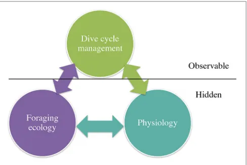
Diving predators need to acquire sufficient resources which among other factors are determined by prey distribution, abundance, and quality. These need to be balanced against their
physiological constraints (e.g., oxygen stores, age/size or sex influencing diving capacity). The interplay between need and constraint is reflected in what is directly observable, and what can be measured, for example, dive behavior using data loggers. How these predators manage their dive cycle structure is the key from which inferences can be made about the “hidden” aspects of foraging and physiology (Figure 1).
In our study, we conducted a systematic literature review of publications using dive telemetry in the Southern Ocean with a focus on 2006–2016 (Supplementary Material), as this was a period of considerable study employing both well established sensors (e.g., time-depth recorders) and emerging techniques (e.g., accelerometry, animal-borne cameras). We searched for peer-reviewed literature, published in English, containing the words: dive data, tag, time-depth recorder, TDR, Southern Ocean, Antarctic, marine mammals, penguins, seabirds, seals, cetaceans, and species names. For identifying SO birds and mammals, we followRopert-Coudert et al. (2014). Most research data is from south of 40◦S (De Broyer and Koubbi, 2014a,b),
although some species are clearly limited to the Antarctic region (i.e., south of 60◦S). This substantial field of telemetry work
comprises 218 studies of 24 species, including 10 species of marine mammals and 14 species of seabirds, that used a variety of different data loggers and sensors. The full literature database is made available underSupplementary Material.
[image:2.595.307.551.501.664.2]Where pertinent, we do refer to literature published outside the 2006–2016 time frame, as key studies obviously occurred either before this decade, or studies were conducted on species similar to those included in this review. We do not intend this as a general review of advances in the bio-logging field (for which see, for example,Halsey et al., 2006a,b, 2007a; Mate et al., 2007; Goldbogen et al., 2013; Balmer et al., 2014; McIntyre, 2014; Ceia and Ramos, 2015; Hussey et al., 2015). Rather we aim to examine the richness of information and insights gained, from relatively simple dive data streams, about the underwater lives of Southern Ocean marine predators. While focusing on
mammals or birds only (e.g.,Goldbogen et al., 2013; McIntyre, 2014; Carter et al., 2016) would allow a more detailed coverage, it is timely for a more holistic perspective of the Southern Ocean. We hope this review provides a useful synthesis particularly for new researchers commencing Southern Ocean biotelemetry research.
First, we briefly cover the main observational platforms used (devices and sensors), and the general coverage across SO species and geographical areas. Following a basic explanation of diving behavior, we then synthesize the literature by adopting a question-driven approach: exploring the foraging and physiological inferences achievable using dive data. Adopting this approach organizes the insights obtained from dive telemetry under an ecological framework which, we suggest, provides a useful context for aligning the analyses of dive metrics. This perspective might thereby serve to facilitate comparative multi-species analyses and meta-analyses. The scope of the review covers what has been learnt about important SO predators, and particularly how tags, data and analytical methods were used. The review closes with a perspectives section considering the outstanding questions being addressed in emergent areas.
OBSERVATIONAL PLATFORMS
Devices and Sensors
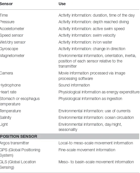
Animal-borne data loggers enable the remote study of various aspects of the biology of free-living animals with regard to behavior, physiology and energetics (Cooke et al., 2004). Data loggers are devices that record information using sensors measuring physical (e.g., light, temperature, or pressure) or physiological properties such as heart rate (Table 1). Measuring the speed at which an animal moves helps, for example, to define the function of the dive (e.g., transit or hunting) (Naito, 2010). More detailed information about an animal’s dive behavior became available with the introduction of sensors, such as gyroscopes (change in direction) (Kawabata et al., 2014), 3-axis magnetometers (orientation) (Friedlaender et al., 2011), cameras (video) (Watanabe and Takahashi, 2013), and hydrophones (sound) (Goldbogen, 2006). Further, recording in situphysical and oceanographic features while an animal is diving provides information of the habitats the animal uses for feeding, and how these may influence vertical distribution of its prey. Finally, recording physiological variables, such as heart rate and body temperature, can provide proxies for metabolism and prey consumption rates (Kuhn et al., 2006; Crossin et al., 2012) (see
Table 1).
[image:3.595.306.551.86.388.2]Throughout the 1970s and most of the 1980s TDRs were predominantly archival, needing to be recovered to retrieve the information. Taking into account difficulties often experienced in recapturing a tagged animal, satellite-linked depth recorders (SLDR) were developed (Bengtson et al., 1993). These typically use the Argos satellite system to relay data which, due the system’s limited bandwidth, often requires high temporal resolution data to be summarized either into user-defined bins (Fedak et al., 2001, 2002) or greatly simplified time depth profiles (e.g., Photopoulou et al., 2015). Satellite-relayed information offers the only solution to studying animals without prospect of recapture,
TABLE 1 |Commercially available sensor types for data loggers and their use for marine mammal and seabird research.
Sensor Use
Time Activity information: duration, time of the day
Pressure Activity information: depth reached diving
Acceletometer Activity information: active swim speed
Speed sensor Activity information: swim velocity
Wet/dry sensor Activity information: in/on water
Gyroscope Activity information: change in direction
Magnetometer Environmental information, orientation, inertia, position of each sensor relative to the transmitter
Camera Movie information processed via image processing software
Hydrophone Sound information
Heart rate Physiological information as energy expenditure
Stomach or esophagus temperature
Physiological information as ingestion
Temperature Environmental information: use of currents
Salinity Environmental information: ocean circulation
Light Environmental information, day/night, seasonality
POSITION SENSOR
Argos transmitter Local-to meso-scale movement information
GPS (Global Positioning System)
Fine-scale movement information
GLS (Global Location Sensing)
Meso- to basin-scale movement information
For further information regarding scales of movement and location errors associated with different positioning sensors see:Bradshaw et al. (2007),Bryant (2007),Block et al. (2011),Costa et al. (2010),Patterson et al. (2010),Winship et al. (2012)and references therein.
such as fledglings, non-breeding individuals and/or those not bound to land (or ice) based colonies.
Usage in Southern Ocean Species
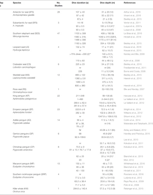
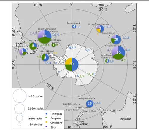
From 2006–2016, data loggers were used to study 24 air-breathing species in the SO: 7 pinnipeds, 7 penguins, 3 cetaceans, and 7 flying seabirds. Most studies focused on pinnipeds (44%) and penguins (41%), while studies on flying seabirds and cetaceans accounted for only 6 and 9% of publications, respectively (Table 2). The reasons for this disparity are likely due to differences in the catchability and accessibility of the different species. More than half of the species studied (n=16) were sub-Antarctic (40–60◦S) species and 8 were high Antarctic species
(>60O S) (Figure 2). The sampling effort was greatest in the South Atlantic.
TABLE 2 |Southern Ocean literature review results showing the number of studies conducted by species from 2006–2016.
Map ID
Species No.
Studies
Dive duration (s) Dive depth (m) References
1 Antarctic fur seal (AFS)
Arctopcephalus gazella
28 107±43 31±20 (12) Arthur et al., 2016
97±42 50±22 (11) Viviant et al., 2016
67±4 21±2 (5) Bestley et al., 2015
2 Subantarctic fur seal (SFS)
A. tropicalis
3 14–18 5–13 (78 p) Verrier et al., 2011
93±0.5 100±0.3 (47)* Luque et al., 2007a 93±0.5 40±0.3 (47) Luque et al., 2008
3 Southern elephant seal (SES)
Mirounga leonina
47 1103±308 409±192 (9) Le Bras et al., 2016
1560±318, 1488±306
1049±315 (326 f), 1170±411 (61 m)
Hindell et al., 2016
1183±326 334±133 (20) Bestley et al., 2015
4 Leopard seal (LS)
Hydrurga leptonyx
4 132±74 17±11 (21) Krause et al., 2016
nr 62±15 (7) Krause et al., 2015
>75% dives<300 (2)** 140±8 (1), 108±7 (1)
Nordøy and Blix, 2009
119±83 44±48 (1 j) Kuhn et al., 2006
5 Crabeater seal (CS)
Lobodon carcinophagus
6 225±23 54±27 (13) Bestley et al., 2015
nr nr (34) Friedlaender et al., 2011
228 11±5.3 (34) Burns and Costa, 2008
6 Weddell seal (WS)
Leptonychotes weddellii
12 489±122 119±38 (18) Bestley et al., 2015
1380±0.6 511±4 (1), Heerah et al., 2015
1260±6 475±4 (1)
600±360 67±54 (1) Heerah et al., 2014
7 Ross seal (RS)
Ommatophoca rossii
1 nr 52–100 (10) Blix and Nordøy, 2007
1 King penguin (KP)
Aptenodytes patagonicus
22 211–248 95–135 (6) Hanuise et al., 2013
1–495 2–344.5 (21) Le Vaillant et al., 2013 269.4±62.4
261.6±57.4
154.8±52.8 (7 f), 143.5±45.4 (8 m)
Le Vaillant et al., 2012
2 Emperor penguin (EP)
Aptenodytes forsteri
23 222.6±6 72.3±4.1 (4) Wright et al., 2014
282±30 102.9±28.6 (7) Williams et al., 2012 nr 1047.8±108.6 (10) Shiomi et al., 2012 3 Adélie penguin (AD)
Pygoscelis adeliae
14 56±4 17.3±1.8 (1) Cottin et al., 2014
97±38, 78±27
nr (14) Watanabe and Takahashi, 2013
Nr 43.08±0.1 (65) Ainley and Ballard, 2012 4 Gentoo penguins (GP)
Pygoscelis papua
6 88 45.9 (20)* Handley and Pistorius, 2015
92.3–109.6 35.9–52.2 (7)
Lee et al., 2015 nr 52.7±16.0 (12) Kokubun et al., 2011 5 Chinstrap penguin (CP)
Pygoscelis antarctica
8 70.5±9
81±13.1 76.7±17.8
29.1±6.6 (20), 37±10.6 (17), 33.9±12.7 (20)
Kokubun et al., 2015
62±25 20±14 (31)* Blanchet et al., 2013
20 5 (2)* Mori, 2012
6 Macaroni penguin (MP)
Eudyptes chrysolophus
13 130±11 48±7 (7) Whitehead et al., 2016
85±36 32±26 (20) Blanchet et al., 2013 40 – 130 9 – 40 (105) Hindell et al., 2011 7 Southern rockhooper penguin (SRP)
Eudyptes chrysocome
4 nr 16±6 (36) Rosciano et al., 2016
77.2±3.5 29.7±3.4 (12) Ludynia et al., 2012 63.2±36.4 20.6±19.4 (4) Raya Rey et al., 2009
71.7±5.5 27.1±5.7 (30) Pütz et al., 2006
1 Killer whale (KW)
Orcinus orca
1 294.6±140.4 57.5±112.5 (9) Reisinger et al., 2015
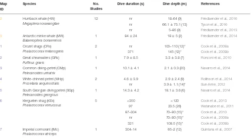
TABLE 2 |Continued
Map ID
Species No.
Studies
Dive duration (s) Dive depth (m) References
2 Humback whale (HW)
Megaptera novaeangliae
12 nr 18–64 (9) Friedlaender et al., 2016
nr 66.1±75.1 (13) Tyson et al., 2016
nr 5–85 (9) Friedlaender et al., 2013
3 Antarctic minke whale (MW)
Balaenoptera bonaerensis
1 84±24 18±5 (2) Friedlaender et al., 2014
1 Crozet shags (CRs)
Phalacrocorax melanogenis
2 nr 100–110 (12)* Cook et al., 2008a
371 145 (12)* Cook et al., 2008b
2 Great shearwaters (GRs)
Puffinus gravis
1 7.9±8.5 3.3±3.8 (7) Ronconi et al., 2010
3 Common diving-petrel (CMp)
Pelecanoides urinatrix
1 10.1±4.1 2.1±0.3 (20) Navarro et al., 2014
4 White-chinned petrel (WHp)
Procellaria aequinoctialis
2 4.6±3.9 2.9±2.4 (9) Rollinson et al., 2014
nr 3.9±1.1 (14)* Sue-Anne, 2012
5 South Georgian diving petrel (SGp)
Pelecanoides georgicus
1 14.3±4.2 18.1±3.6 (6) Navarro et al., 2014
6 Kerguelen shag (KEs)
Phalacrocorax verrucosus
5 <350 <120 Cook et al., 2013
97 23.5 (26) Watanabe et al., 2011
87–304 70–80 (15)* Cook et al., 2010
nr 70–80 (15)* Cook et al., 2008a
321 108.5 (15)* Cook et al., 2008b
7 Imperial cormorant (IMc)
Phalacrocorax atriceps
1 304–14 65–2 (12) Quintana et al., 2007
Examples of reported mean dive durations (sec) and mean depths (m) are given as mean±SD or range (min–max) as available. Sample sizes are given in brackets. For species with few studies (≤5) all references are given here, otherwise the three most recent studies are shown. Abbreviations: nr, numeric value not reported; m, males; f, females; p, pups; j, juveniles. In some case multiple values are given for separate seasons. The full database containing all literature references (n=218) is made available underSupplementary Material.*Indicates mean maximum dive depth was reported;**binned data from satellite-linked recorders.
Peninsula or near the coast on the sea ice, and occasionally on sub-Antarctic islands. Access to these dispersed ice-affiliated species remains challenging over large areas of the SO. Some 80% of studies on Adélie penguins (Pygoscelis adeliae) were carried out in Adélie Land. Macaroni penguins (E. chrysolophus) were most commonly tagged at South Georgia and sub-Antarctic islands within the Indian sector. A few rockhopper penguin (Eudyptes chrysocome) colonies off Argentina and the Falkland Islands fall within the Southern Ocean (i.e.,<40OS). Chinstrap penguins (P. antarctica) were studied at sub-Antarctic islands including South Georgia, South Orkney (Takahashi et al., 2003), and South Shetland (Croll et al., 2006). Finally, emperor penguins (Aptenodytes forsteri) were studied at various colonies along the coast of the Antarctic continent (Wienecke et al., 2007). Albatrosses and diving petrels were studied at South Georgia and the South Orkney Islands (Phillips et al., 2005, 2007; Rollinson et al., 2014). The only site where the diving ability of cormorants (Phalacrocoraxspp.) was studied in the last 10 years is the Crozet archipelago (Cook et al., 2008a,b). For cetaceans, the studies were carried out near the Auckland Islands, the Falkland Islands and in South America, and in the Antarctic Peninsula region.
Cetacean telemetry studies have lagged somewhat behind those of seals and penguins largely due to accessibility, as well as technological issues with tag attachments. These are resolving and beginning to provide valuable longer term tracking datasets (e.g.,Reisinger et al., 2015; Weinstein and Friedlaender,
2017). Additionally, the tag design for DTAGs (multisensor archival digital acoustic recording tags,Johnson and Tyack, 2003; Goldbogen et al., 2013) provides some of the most sophisticated diving data achievable for the study of free-living animals, albeit still usually at short time scales (typically a day or so, using suction cup attachments, e.g.,Tyson et al., 2016). Taking these developments into account we can expect a maturation of this field and consequent major expansion of these data over the next decade. The study of SO seabirds also largely remains focused on movement studies, often with the addition of simple wet/dry activity sensors (e.g.,Phalan et al., 2007). Seabird diving studies continue only in relatively low numbers, but we may similarly expect an increase in future with the ongoing miniaturization of data loggers and sensors.
THE BASICS OF DIVING BEHAVIOR
FIGURE 2 |Spatial distribution of sampling effort/data logger deployment in the Southern Ocean during 2006–2016 for each species. Circle size and white number represent the total number of studies carried out in each location. Color-coded numbers correspond to the species cited inTable 2. The database containing all literature references is made available underSupplementary Material.
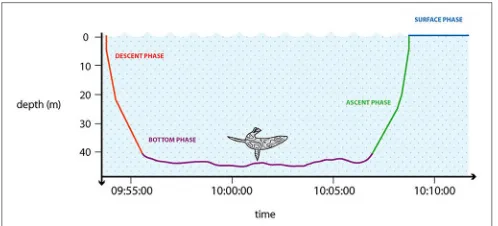
Each dive can be divided into distinct phases (Figure 3). The descent phase (DESC) represents a period of active swimming using sequential, large amplitude strokes of flippers, flukes or feet to reach the desired depth (Williams et al., 2000). The bottom phase (BOT) is defined as the period between the dive descent and ascent. Often this is simplified as the time between the first and last recorded depth that is some fraction (e.g., 80%, but also 60–85% depending on the species) of the maximum depth (Austin et al., 2006; Bailleul et al., 2008). Halsey et al. (2007a) proposed the definition as between the first and the last wiggle or step, being deeper than a given proportional depth threshold, assigned per species. The bottom phase is generally assumed to be connected to feeding activity. During
FIGURE 3 |Stylized graphic representation showing a general dive of a marine predator. The diving phases are summarized using different colors: descent phase (red); bottom phase (violet); ascent phase (green); surface phase (blue). Designed by: Charlie Armstrong.
On the basis of their profiles, dives may be classified typically as square dives (DESC =ASC with BOT); V-shaped (DESC = ASC without BOT); skewed right (DESC < ASC) or left dive (DESC > ASC) (Schreer et al., 2001). Among all species and groups, square dives are generally regarded as foraging dives, although Weddell seals may use V-shape dives for feeding (Fuiman et al., 2007). In contrast, left and right skewed dives generally have a different purpose and are usually performed during traveling and searching activities. However, among elephant seals skewed right dives may be linked with food processing (Crocker et al., 1997).
Individual dives often occur in clusters or bouts. Bouts as defined by Boyd and Croxall (1992) are: “a series of four or more dives not separated by a surface period exceeding a few minutes.” The end of a bout is derived from the post-dive surface interval of the last dive, but can be difficult to determine. Luque and Guinet (2007b)suggested that employing a maximum likelihood estimation method delivers the most accurate means to determine when a bout has ended. Bout durations and locations can provide information on the spatial scale of prey patches (Mori, 2012), as the animal moves between successive patches (Hooker et al., 2002). Information about bouts can also be used to make inferences about foraging preferences (e.g., prey type, Elliott et al., 2008), or foraging effort (Della Penna et al., 2015).
A trip comprises the entire time an animal spends at sea from the time it leaves land (or sea ice) to the time it returns; generally many dive bouts are performed during this period. Depending on the species and breeding status, trips may range from several days to many weeks, and short and long trips may be alternated (e.g.,Chaurand and Weimerskirch, 1994; Croxall and Davis, 1999; Luque et al., 2007a; Green et al., 2009a). At the Kerguelen and Crozet islands, rockhopper penguins performed daily trips during the brooding period, but as chicks grew older trip durations increased (Tremblay and Cherel, 2005). For some taxa, such as cetaceans or pack-ice seals, the concept of a trip is not necessarily as well defined but can be regarded as the time spent moving between regions to which they demonstrate some fidelity. For example, Antarctic seal-hunting (B type) killer whales (Orcinus orca) from the Antarctic Peninsula make
periodic round trips to the South American coasts and back probably for physiological maintenance rather than for feeding or breeding purpose (Durban and Pitman, 2012).
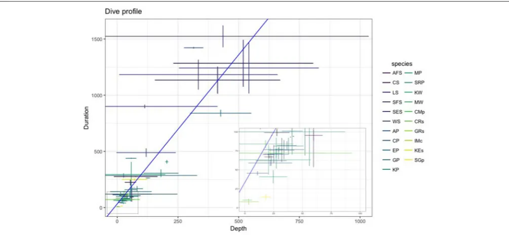
Multiple factors including body condition (e.g.,Miller et al., 2012; Richard et al., 2014; Gordine et al., 2015), age (Le Vaillant et al., 2012, 2013), sex (Beck et al., 2003; Baird et al., 2005), life history stage (Schulz and Bowen, 2004; Verrier et al., 2011), and body size (Irvine et al., 2000; Mori, 2002; Navarro et al., 2014) can all influence an animal’s diving behavior. An example of how dive capabilities (depth and duration) vary across SO species is presented in Figure 4. In general, larger seabirds and marine mammals dive longer and deeper than smaller species (Schreer et al., 2001). However, there are exceptions: for example, among petrels and albatrosses, smaller species tend to diver deeper in relation to their body mass than larger species (Prince et al., 1994; Navarro et al., 2014).
FORAGING INFERENCE
Southern Ocean predators use diverse habitats and feed on a wide variety of prey. By understanding the diving behavior of these species we are able to address a number of key ecological questions including: What is the distribution of their prey (spatial, vertical, among habitats, and seasonally)? What is their prey type (schooling/individual, benthic, or pelagic)? What are the foraging strategies adopted? What is the prey density (relative abundance) and quality? How much is eaten? Ultimately, integrating these observations can help explain the foraging activity and success for individual animals in time and space, as well as their functional response when facing environmental changes.
Prey Distribution and Type
FIGURE 4 |The relationship between dive duration (s) and depth (m) across the most commonly researched SO marine predators described inTable 2(species abbreviations given in table). Values shown as mean±SD. Inset panel provides a closer look at shorter (<100 s) and shallower (<100 m) dives. Data collected from studies undertaken between 2006–2016 (seeSupplementary Material).
Adélies and feed inshore, while Adélies forage farther offshore (Takahashi et al., 2003). Interpretation of pelagic and benthic foraging behavior clearly requires a spatial context and may be hampered by poorly resolved bathymetry.
The size of prey items consumed by an animal is highly variable and not linearly related to the body size of the predator. For example, some marine predators ingest very large numbers of small prey items at a time (e.g., whales feeding on krill swarms; Kawamura, 1994) while others chase a single large prey item (e.g., Weddell seals eating large lipid-rich toothfish;Ainley and Siniff, 2009). The diet of marine mammals and seabirds has traditionally been studied through of the enumeration of stomach contents and/or scats, and is increasingly approached though methods, such as fatty-acid analyses (Pierce and Boyle, 1991), stable isotope signatures (Cherel et al., 2007; Cherel, 2008) and DNA-based methods (Deagle et al., 2007; McInnes et al., 2016, 2017). Such information may be powerfully integrated with tracking data to provide a spatial context (e.g.,Bailleul et al., 2010; Walters et al., 2014), and dive data may also be used to infer what SO species consume (Hocking et al., 2017).
Dive bout duration and inter-bout intervals can provide a relative indication of the size of prey patches and dispersion of prey types (Boyd and Croxall, 1996; Mori, 1998). Depending on the particular predator and prey combination, a bout may correspond to a single or multiple prey patches. Bout types or structures may be differentiated by combined parameters, such as timing (day/night/dusk), length (short/long), and depth (shallow/deep) (e.g., Boyd et al., 1994; Lea et al., 2002), and can help discriminate the prey item(s) that are being targeted by a predator (e.g., Elliott et al., 2008). Bout duration and timing between bouts can provide information on the temporal
distribution of foraging patches (Luque et al., 2008). In a study of provisioning Adélie penguins,Watanuki et al. (2010) found longer dive bouts tended to occur toward the end of foraging trips, and were associated with higher meal mass. Combined information on dive depth distribution and dive bout characteristics (e.g., proportion of dives in a bout, number of dives per bout, bout type) can identify prey as being epipelagic (e.g., surface-swarming krill;Lee et al., 2015), or mesopelagic (e.g., myctophid fish and cephalopod species; Georges et al., 2000), and whether prey are more aggregated (high number of dives per bout) or dispersed (low number of dives per bout) (Lea et al., 2002).
exploiting shallow schools of silverfish. However, animal-borne videos typically represent short observation periods relative to other behavioral records, and efficient image storage and processing methods are currently an active area of research.
Foraging Strategies
Optimal foraging theory (OFT) (Stephens and Krebs, 1986) is a conceptual framework widely employed to examine the strategies animals use to acquire food. Under the OFT framework, animal movement and behaviors are expected to be as efficient as possible. Translated to air-breathing divers, OFT suggests these animals should minimize the costs associated with feeding underwater (e.g., dive transit time, oxygen consumption) and maximize the benefits using some fitness related criterion (e.g., time spent at foraging depths, net energy gain or energy efficiency, load size, prey capture rate) (Kramer, 1988; Houston and Carbone, 1992; Mori, 1998). The most commonly developed dive optimality models are “time allocation models” (Houston, 2011) that seek to optimize the foraging and surfacing time of animals in response to changing conditions, such as prey depth (Mori and Boyd, 2004) or prey encounter rate (Thompson and Fedak, 2001). In the latter case, Thompson and Fedak (2001) investigated the effects of a “giving up” rule to demonstrate cases where a net benefit was obtained by terminating dives that are likely to be unproductive. While this general held true for shallow divers, it was unclear for deep divers such as southern elephant seals. Moreover, in the controlled environment of captive experiments where the model was tested on gray seals (Halichoerus grypus), it was not clear if the effect held true in all situations (Sparling et al., 2007).
Time-depth recorders and other bio-logging tools such as accelerometers have allowed OFT models to be developed, and predictions tested, across a wide array of free-ranging marine predators. A non-exhaustive list of applications to SO species include Antarctic fur seals (Mori and Boyd, 2004), southern elephant seals (Gallon et al., 2013), Adélie penguins (Watanabe et al., 2014), macaroni and gentoo penguins (Mori and Boyd, 2004), king penguins (A. patagonicus) (Hanuise et al., 2013), humpback (Megaptera novaeangliae) (Tyson et al., 2016) and fin (Balaenoptera physalus) whales (Acevedo-Gutiérrez et al., 2002; outside SO). The results ofAcevedo-Gutiérrez et al. (2002), who compared observed TDR dive times to those predicted by an OFT model, suggested that the foraging strategies of fin whales are energetically expensive and limit the dive time of these large predators. More recently,Tyson et al. (2016)tested a suite of OFT models for humpback whales foraging at the western Antarctic Peninsula using high-resolution multi-sensor data loggers. They found that the agreement between observed and optimal behaviors varied widely depending on the physiological and behavioral values used to derive optimal predictions, and highlighted the need for an improved understanding of cetacean physiology.
In their seminal paper,Mori et al. (2005)used an optimality framework to derive prey indices from Weddell seal diving profiles, in conjunction with prey richness estimates from animal-borne camera data. The authors generally found positive correlations between these two indices (dive profiles and prey
richness), but highlighted the importance of identifying the relationship between the diving behavior of predators and the type of prey they take (see above) in order to estimate prey abundance using diving profiles. Smaller numbers of larger prey are sufficient in terms of energy intake; for example, a single large high-quality items such as Antarctic toothfish (Dissosichus mawsoni) delivers possibly more energy per ingestion than smaller prey like Antarctic silverfish which may require several dives to obtain the same amount of biomass comparable to a single toothfish. However, there may be an increased energetic cost when digesting one large prey item whose temperature is much lower than that of the predator’s core (see Prey consumption, below).
Dive profiles can also provide more general information on predation strategies, for example whether foraging animals approach their prey from above or below. Using a time-depth-speed logger,Ropert-Coudert et al. (2000)reported steep acceleration events where king penguins swam rapidly upwards mainly during the bottom and early ascent phases of dives. This appears to reflect an upward-looking attack strategy, whereby prey is detected and approached from below. It is likely that multiple prey approach and capture techniques are employed by individuals, depending on factors, such as light, bioluminescence and seasonal progressions in prey type, and abundance and density. Antarctic marine predators seem to employ active-search hunting rather than ambush (sit-and-wait) strategies, although a passive-gliding approach from above the prey target has been recently documented in elephant seals (Jouma’a et al., 2017). Using time-depth data in conjunction with animal-borne video, Krause et al. (2015) reported novel observations on foraging leopard seals such as unique prey-specific hunting tactics when targeting Antarctic fur seal pups and fishes including stalking, flushing, and ambush behaviors.
Prey Density and Quality
Drawing mainly from the OFT framework, a large research effort has focused on developing indices from diving telemetry data of predators that can provide information on prey quality or density.
important predictor of dive behavior (e.g., Thums et al., 2013; Richard et al., 2014; Jouma’a et al., 2015).
Similarly, a straightforward interpretation under an optimality framework might expect maximized time spent at the bottom of a dive to represent greater prey density and/or quality and enhanced foraging benefit for marine predators. Many indices have been derived to investigate bottom time relationships (Table 3) attempting to account for deeper dives in the water column that necessarily take more time, with less time subsequently to be spent at the bottom. These include dive residuals (Bestley et al., 2015), residual bottom time (Dragon et al., 2012), and residual “first bottom time” (Bailleul et al., 2008). The latter attempts to translate classical first passage time (Fauchald and Tveraa, 2003), widely used to analyse area-restricted search in horizontal movements, into the vertical dimension.
Validation with external datasets has not clearly resolved whether longer bottom phases are indicative of higher or lower prey quality or density, and hence foraging success. For example, short-term measurements of head jerks in southern elephant seals using accelerometers suggested increased prey capture attempts with increased bottom durations (Gallon et al., 2013). However, in Antarctic fur seals, the relationship between head jerks and dive metrics—including bottom duration—varied markedly with temporal scale (i.e., dive to all-night scale) (Viviant et al., 2014). In a related study, Viviant et al. (2016) showed Antarctic fur seals adjust their time in the dive bottom phase mainly according to prey patch accessibility (depth) and their physiological constraints (behavioral aerobic dive limit), rather than their prey encounters (mouth-opening events). In king penguins, heart rate loggers showed increased heart rates, and hence energetic costs, associated with shorter dive durations, shorter bottom times, and longer surface durations (Halsey et al., 2007b). Similar patterns in elephant and Weddell seals appear to represent high activity dives in higher quality areas (Bestley et al., 2015). Furthermore, faster descent speeds, shorter dive durations, and reduced bottom times in higher-quality habitat were linked to body condition indices of elephant seals (Thums et al., 2013). Longer dive and bottom durations occurred when patches were of relatively low quality consistent with the predictions of the marginal value theorem (MVT,Charnov, 1976). Qualitative support for the MVT has also been provided for Adélie penguins, with opposing effects of patch-quality on duration at the dive- (positive) and bout- scale (negative), respectively (Watanabe et al., 2014). The way predators balance their dive budgets in terms of transit speed, bottom duration, and surface intervals is likely a function of interacting factors, such as the quality, size, vertical distribution and behavior of the prey, and the optimal approach will be changeable with prey-switching as discussed above. Bottom durations may also differ markedly between habitats—benthic, epipelagic or midwater— with potentially longer bottom phases during benthic dives (e.g., gentoo penguins, seeKokubun et al., 2010).
The complexity of diving depth profiles has been widely investigated to make inferences about feeding activities. In particular, the vertical undulations or “wiggles”—changes in swim direction occurring at depth—are indicators of prey
encounter rates or prey capture attempts. These are commonly simply counted (e.g., Bost et al., 2007), although a number of metrics have been developed to evaluate vertical sinuosity of dives (e.g., Dragon et al., 2012) and optimally allocate segments within dives as “hunting” or “transit” time on the basis of sinuosity thresholds (e.g., Heerah et al., 2014, 2015). Validations of such depth variations as feeding proxies have been based on various external measurements including oesophageal temperature (Adélie and king penguins, Bost et al., 2007), stomach temperature (southern elephant seals,Horsburgh et al., 2008), and accelerometers to detect mouth opening events (king penguins,Hanuise et al., 2010; Antarctic fur seals,Viviant et al., 2014). These studies generally reported good correspondence between dive profile variations and other more direct measures of feeding activity. However, not all vertical undulations are prey encounters, not all encounters have an undulation, and only a proportion of prey encounters result in capture and ingestion. Consequently, in free-living animals it remains difficult to validate the actual success of prey encounters or capture attempts as unsuccessful attempts may still result in ingestion of cold water. Thus, the above mentioned variables ought to be considered mainly as indicators of forage effort rather than forage success.
Prey Consumption
A key question with regard to dynamics of ecosystems is how much food is eaten by marine predators. To obtain actual information on foraging success requires ancilliary data to simple dive traces. Short-term direct observations of feeding activity can be obtained with tag-mounted cameras (Mori et al., 2005; Watanabe and Takahashi, 2013). As mentioned briefly above, methods like stomach or oesophageal temperature sensors for seabirds (Bost et al., 2007, 2015; Hanuise et al., 2010) and seals (Austin et al., 2006; Horsburgh et al., 2008; Kuhn et al., 2009) can provide information on prey capture attempts; since birds and mammals in the SO have a higher core body temperature than their prey, their stomach temperature drops during ingestion (Wilson et al., 1992). However, unsuccessful attempts may still result in ingestion of cold water and need to be clearly distinguished from successful feeding events. Head or jaw mounted accelerometers and speed sensors have also been used to provide feeding proxies in several seal species (Weddell,Naito et al., 2010; Antarctic fur,Iwata et al., 2012; southern elephant, Gallon et al., 2013; Guinet et al., 2014; Richard et al., 2014; Vacquié-Garcia et al., 2015), and penguins (king,Hanuise et al., 2010; chinstrap and gentoo,Kokubun et al., 2011).
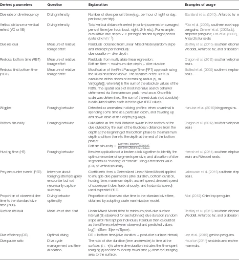
TABLE 3 |Examples of derived dive parameters to investigate diving patterns, foraging behavior, and physiology of SO marine predators.
Derived parameters Question Explanation Examples of usage
Dive rate or dive frequency Diving intensity Number of dives per unit time (e.g., per hour of night or day; per bout; per trip).
Staniland et al. (2010), Antarctic fur seals.
Vertical distance or vertical extent (VD or VE)
Diving intensity Total vertical distance traveled (m or km) summed or averaged per unit time (per hour, bout, night, 24 h etc.). For example: cumulative dive depth×2 per night divided by night period (units of km h−1)
Pütz et al. (2006), southern rockhopper penguins;Zimmer et al. (2008a,b), emperor penguins;Lea et al. (2002), Antarctic fur seals
Dive residual Measure of relative forage effort
Residuals obtained from Linear Mixed Model (random slope and intercept per individual):
dive duration∼dive depth
Bestley et al. (2015)southern elephant, Weddell, Antarctic fur, and crabeater seals.
Residual bottom time (RBT) Measure of relative forage effort
Residuals from multivariate linear regression: Bottom time∼maximum dive depth+dive duration
Dragon et al. (2012)southern elephant seals.
Residual first bottom time (rFBT)
Measure of relative forage effort
Modification of the First-Passage Time (FPT) approach using the RBTs described above. The variance of the RBTs is calculated within circles of increasing radius (r), as
Var[log(t(r))], where t(r) is the sum of the absolute values of the RBTs. The spatial scale of most intensive search behavior determined via the maximum peak in variance. Once this scale was determined, the sum of the residuals (not absolute) is calculated within each circle to give rFBT values.
Bailleul et al. (2008)southern elephant seals.
Wiggles Foraging behavior Detected as anomalies in diving profiles: when an animal is spending some time at a particular depth, and traveling up and down while at this depth (zig-zags).
Hanuise et al. (2010)king penguins.
Bottom sinuosity Foraging behavior Calculated as the total distance swum in the bottom of the dive divided by the sum of the Euclidean distances from the depth at the beginning of the bottom phase to the maximum depth and from there to the depth at the end of the bottom phase:
Bottom sinuosity=Bottom Distanceobserved Bottom Distanceeuclidean
Dragon et al. (2012)southern elephant seals
Hunting time (HT) Foraging behavior Iterative application of a broken stick algorithm to identify the optimum number of segments per dive, and allocation of dive segments as “hunting” or “transit” using a threshold value (0.9) of vertical sinuosity.
Heerah et al. (2014)southern elephant seals and Weddell seals.
Prey encounter events (PEE) Inference about foraging attempts (prey encounter but not necessarily capture success)
Coefficients from a Generalized Linear Mixed Model applied to multiple dive parameters (dive duration, bottom duration, hunting-time, maximum depth, ascent speed, descent speed of subsequent dive, track sinuosity, and horizontal speed) used to predict PEE.
Labrousse et al. (2015)southern elephant seals.
Proportion of observed dive time to the standard dive time (POS)
Diving behavior optimality
Proportion of observed dive time to the standard dive time, obtained by adopting a rate maximization model.
Mori (2012)Chinstrap penguins
Surface residual Measure of dive cost Linear Mixed Model fitted to minimum post-dive surface interval (SI) observed for each (binned) dive duration (random slope and intercept per individual). Residual then calculated as the difference between observed and predicted values: log(1+(SIobs–SIpred)/SIpred).
Bestley et al. (2015)southern elephant, Weddell, Antarctic fur, and crabeater seals.
Dive efficiency (DE) Optimal diving DE=bottom time/(dive duration+post-dive surface interval) Lee et al. (2015)gentoo penguins. Dive:pause ratio Dive cycle
management and time allocation
The ratio of dive duration (time underwater) to time at the surface: (t+τ)/s where dive duration includes the time spent foraging (t) and the round trip travel time (τ) from the foraging area to the surface.
Houston (2011)seabirds and marine mammals.
these events for low-resolution dive profiles available over longer periods. Informative variables included ascent speed, maximum depth, bottom time, and horizontal speed (pelagic strategy), compared with just ascent speed and dive duration (demersal strategy).
These modeling approaches may greatly increase the utility of both data types and provide some indicator of feeding activity over whole migration trips. However, information on actual
into the location and charactersitics of successful Southern Ocean foraging areas (Biuw et al., 2007; Hindell et al., 2016), and was incorporated into population-level models integrating the physiological and movement ecology of predators (Schick et al., 2013; New et al., 2014). Efforts have been made to validate relationships between descent rates and drift rates (Richard et al., 2014), which represent a promising extension of inference to basic dive profiles and potentially broader application across other species. A recent study on Antarctic fur seals ( Jeanniard-du-Dot et al., 2017) incorporated information of prey capture attempts into an energetics framework to estimate foraging efficiency and the consequences for reproductive success (pup growth). Such applications, linking individual foraging behavior with demographic consequences (see alsoHiruki-Raring et al., 2012), are important avenues for future biotelemetry research in the Southern Ocean.
Overall, relatively simple dive data streams continue to provide increasingly powerful insights into marine predator foraging. However, when used alone these telemetry data remain largely limited to providing information on effort. Dive metrics cannot confirm success; indeed dive metrics (e.g., residuals: positive and negative from a fitted relationship) may be obtained from an animal that in fact fails to forage at all. Combined usage of TDRs with other devices that provide more direct observations (e.g., accelerometers, miniature cameras, speed turbines, internal sensors), even on a subset of individuals, greatly assists in maximizing inference. In addition, the caveats of inferring from dive data may be alleviated by combining data from different sources, such as isotopes and DNA methods (diet), mass or lipid gain (success), reproductive outputs (energetic costs) thereby achieving a broader perspective on the foraging of Southern Ocean marine predators.
INTRINSIC DETERMINANTS OF
DIVING—PHYSIOLOGICAL INFERENCE
The foraging strategies adopted by marine predators are not only dictated by prey abundance and distribution but also by intrinsic factors, such as oxygen stores, metabolism, body size, and age (Kooyman and Ponganis, 1998; Costa, 2007; Ponganis et al., 2009; Ponganis, 2011; Castellini, 2012; Elliott, 2016). Relatively few data have been collected on the at-sea metabolism of marine birds and mammals given the practical difficulties of collecting respiration and activity data in the field. Consequently, much of what is known has been inferred from simple dive data. Information on dive duration and post-dive surface intervals provide valuable insights into diving metabolic rate, and on how animals balance time underwater using oxygen stores with time on the surface replenishing them, i.e., dive cycle management. Determining how these intrinsic factors scale with size, sex or age of the animal are key questions that remain largely unanswered. This section discusses how the use of classic dive data information provides valuable insights into dive energetics and the physiological adaptations of SO marine animals, drawing also upon examples from temperate species in a few cases.
Physiological Determinants and
Constraints
Castellini (2012)and Ponganis and Kooyman (2000) reviewed the physiological adaptations among marine mammals and polar seabirds, respectively. We provide a summary here as a base for the following discussion. Many animals dive, but deep divers face a number of challenges, such as the increase in pressure with the resulting mechanical compression of tissue and gas-filled spaces, and the lack ofad libitumaccess to oxygen (Kooyman and Ponganis, 1998; Costa, 2007; Ponganis, 2011). The former is to some extent dealt with using morphological adaptations, such as flexible rib cages (e.g.,Cozzi et al., 2010) and collapsable lungs (e.g.,Falke et al., 1985; McDonald and Ponganis, 2012), while the lack of continuous access to oxygen requires a complex suite of physiological adaptations.
A number of adaptations evolved convergently among marine mammals and seabirds to enable deep diving, but there are also important differences, for example with regard to the distribution of oxyen stores in the body and the reliance on anaerobic metabolism (see below). These animals depend on adaptions that increase intrinsic oxygen stores. Body size is one factor which influences both oxygen storage and metabolic rate or oxygen use (e.g.,Noren and Williams, 2000). Furthermore, to expand their breath holding capacity, deep divers have large volumes of blood. For example, in Weddell seals about 14% of their body weight is due to blood; this is 63 l for a 450 kg seal, or 140 ml kg−1 (Zapol, 1996). In comparison, in humans blood makes up only about 7% of body weight (Zapol, 1996). In penguins, the blood volume is less than in seals; emperor penguins comprise about 100 ml blood per kg body weight (Ponganis et al., 1997a), and for Adélie penguins the value is about 93 ml kg−1(Lenfant et al., 1969).
respectively, and only 19% in the respiratory system (Kooyman and Ponganis, 1998).
The regulation of oxygen use during dives underlies complex physiological processes and depends on a variety of factors, such as dive depth and duration, level of muscle activity (Hindle et al., 2010), and body temperature (Kooyman and Ponganis, 1998). Air-breathing diving vertebrates adjust oxygen consumption through a process known as the “dive response,” a process characterized by a drop in heart rates, decreased blood perfusion of organs (except the brain) and a drop in body temperature (Butler and Woakes, 2001); the result is an overall reduction of oxygen consumption. The dive response essentially manages how long an animal can stay submerged, how much oxygen it has available, and the rate at which this oxygen is consumed. Since in deep diving endotherms a great concentration of oxygen is stored in the muscles (see above), the reduction of the blood flow causes a hypoxia facilitating the oxygen dissociation from myoglobin. This mechanism enhances aerobic metabolism in exercising muscles, despite the reduced blood flow during diving (Davis, 2014). If oxygen stores become depleted during a dive, animals can switch to anaerobic metabolism. However, anaerobic production of energy (glycolysis) is less efficient than aerobic pathways as less adenosine triphosphate (ATP, high-energy molecule) is produced and the muscle tissues accumulate lactic acid. Excessive amounts of lactic acid result in metabolic acidosis and consequently severe depression of the heart and the central nervous system (Wildenthal et al., 1968; Siesj, 1988). To remove lactic acid the animal must pay an oxygen debt. This is commonly achieved by spending extended periods at the surface to re-oxygenate tissues (Kooyman et al., 1980) which in turn can reduce foraging time and limit opportunities (Butler, 2006). However, it can be advantageous for individuals to incur such a metabolic debt.
The change from aerobic to anaerobic metabolism is determined by the Aerobic Dive Limit (ADL), i.e., the time an animal can remain submerged before levels of lactate exceed those present when an animal is resting (Kooyman, 1985). Post-dive partial pressures of oxygen in venous blood (PO2) were measured in free-living Weddell seals and bottlenose dolphins (Tursiops truncatus) and ranged from 15–20 mmHg (Ridgway et al., 1969; Ponganis et al., 1993) which is less than the values obtained from terrestrial mammals after intense exercise (27– 34 mmHg; e.g.,Taylor et al., 1987). Among free-diving emperor penguins, PO2 levels were <20 mmHg in 29% of dives and even dropped to 1–6 mmHg at times (Ponganis et al., 2007). Blood oxygen stores were also nearly completely exhausted in northern elephant seals (M. angustirostris) in whom venous PO2 was recuded to 2–10 mmHg after dives that lasted>10 min (Meir et al., 2009). To withstand such extreme levels of hypoxemia various adaptations such as an enlarged density of capillaries are necessary, but these are not yet fully understood (Ponganis et al., 2007). Some species constantly exceed their estimated ADL. In a review of 6 marine predators at South Georgia, all species except Antarctic fur seals (≤5%), frequently surpassed their estimated ADL (Boyd and Croxall, 1996). Benthically feeding otariids [e.g., Australian sea lions (Nephoca cinerea)] tended to exceed their ADL more often than pelagically foraging species (e.g., Antarctic
fur seals,Costa et al., 2004). Female southern elephant seals went beyond their calculated ADL in 40% of dives, in comparison with only 1% in males (Hindell et al., 1992). Emperor (20% of dives,Butler, 2004), king (20% of dives,Kooyman et al., 1992) and gentoo penguins (40–50% of dives, Williams et al., 1992) also regularly exceeded their ADL, as did Macquarie shags (P. purpurascens) (e.g., 19% of male dives, Kato et al., 2000) and blue-eyed shags (36% of dives; Boyd and Croxall, 1996). The pattern of few anaerobic dives observed among fur seals might be consistent with the maintenance of a high metabolic rate while diving, whereas the bimodality observed in other species suggests fundamentally different strategies may be used to regulate oxygen consumption between short and long dives (Boyd and Croxall, 1996). More recent work has focused on anatomical adaptions and dive capacity (Meir et al., 2008;Ponganis et al. 2009; 2010b; Wright et al., 2014). However, little has been done to empirically determine the ADL for any Southern Ocean species.
Longer post-dive surface intervals do not always indicate an oxygen debt. Even after aerobic dives, the time required to re-oxigenate tissues may be longer after extended dives due to the mechanical restrictions of respiration and airway structure. The “dive:pause ratio” measures the ratio of dive duration to time at the surface. Larger ratios indicate that post-dive surface intervals are long relative to the dive, reflecting the relatively greater time required to replenish oxygen stores. Cormorants have to spend more time at the surface after longer dives, resulting in a dive:pause ratio equal to 1 (Lea et al., 1996). Gentoo penguins have a dive:pause ratio for deep dives of 1.2–2.2 and of 0.3–0.4 for shallow dives (Williams et al., 1992).
Elephant seals did not have appreciably longer surface intervals even for the longest dives; irrespective of the preceding dive, surface intervals last typically only 2–3 min (Hindell et al., 1992). This was considerably shorter than the 50 min surface intervals made by Weddell seals known to have exceeded their ADL (Kooyman et al., 1980). This provides strong evidence that many, if not all, of the female elephant seal dives that surpassed their calculated ADL were in fact aerobic. Thus, the diving metabolic rate of elephant seals may be less than the allometrically derived estimates of metabolic rate used in the calculation of the ADL. Reduced metabolic rate during diving is a well-known consequence of the dive reflex, and the simple metric of dive depth and PDSI can be used to infer the magnitude of this reduction, at least in aerobic dives. The estimate of the metabolic rate in emperor penguins, which was relatively low when foraging, could be used to calculate with a better approximation the ADL for this species than the O2 store data (Nagy et al., 2001). This has implications for energetic models commonly used in ecosystem and fisheries models, as deep diving predators may use less energy than expected from allometric estimations.
insights into the mechanisms that underpin the dive response. Simple time depth data are insufficient to demonstrate some types of behaviors, but augmentation with an additional sensors (such as velocity from accelerometers) expands the capacity for inference. For example, accelerometers in combination with TDRs revealed that southern elephant and Weddell seals use strategies, such as passive sinking and burst-glide swimming, to reduce their oxygen consumption during diving (Hindell et al., 2000; Williams et al., 2000). Kerguelen shags (P. verrucosus) adapt their stroking activity depending on the body buoyancy variation (Cook et al., 2010). A similar mechanism is used by cetaceans (whales,Acevedo-Gutiérrez et al., 2002; dolphins,Williams et al., 2017).
Behavioral Mechanisms as Proxies for
Physiological Mechanisms
An animal’s buoyancy plays an important role in diving; increased buoyancy provides challenges for animals during descent and is energetically expensive, given that animals require additional work, for example, to maintain their position in the water column (Webb et al., 1998). However, buoyancy varies at a range of temporal scales, firstly within an individual annual cycle (e.g., gestation in elephant seals, Crocker et al., 1997) and also throughout its life as an animal grows and develops different traits (e.g., becoming a dominant male for elephant seals,Galimberti et al., 2007). Buoyancy can, however, also be used as a measure of an animal’s body condition because lipids are less dense than water making fatter animals more buoyant than leaner conspecifics (Miller et al., 2012). Some species perform “drift” dives where they stop swimming and are stationary in the water column. The rate and direction of drift has been related to the animal’s total lipid content at that time (Biuw et al., 2003). This means that spatio-temporal dynamics of lipid gain (and loss) can be measured, identifying regions of poor and good foraging. An analysis of elephant seal drift data from many of the major breeding sites indicated that some regions such as the Antarctic Circumpolar Current frontal systems in the Atlantic sector may be better quality habitat than other sectors of the SO. For example, seals from the declining Macquarie Island population had to travel for over a month to reach prime habitats (Biuw et al., 2007). Finer-scale measurements of burst and glide behavior have also been used to measure changes in buoyancy, opening the use of this approach to a wide range of species (Williams et al., 2000; Oliver et al., 2013; Jouma’a et al., 2015).
Tri-axial accelerometers were employed to measure overall dynamic body acceleration (ODBA) which is considered a proxy for energy expended by animals during different diving phases (Wilson et al., 2006; Gleiss et al., 2011). Acceleration is used to measure movement, and since muscle motion involves oxygen consumption, acceleration could be used as a proxy for O2consumption itself. When foraging, Magellanic penguins descended faster than they ascended, which means their descent phase was energetically much costlier than their return to the surface (Wilson et al., 2010). Previous studies conducted on cormorants and pinnipeds have shown how ODBA offers a better estimation of energy expenditure than doubly labeled water
method (Wilson et al., 2006; Fahlman et al., 2008) or flipper stroke evaluation (Jeanniard-du-Dot et al., 2016). However, ODBA is best used for quantifying energy during individual diving phases only rather than the full foraging trip (Wilson et al., 2010) because it might be affected by animal mass, number of strokes, and the relationship between heart rate and O2 consumption (e.g., change of heart rate during dive response).
Other sensors can measure an animal’s physiology more directly. Heart rate can be measured with externally (Hindell and Lea, 1998; Elmegaard et al., 2016) or subcutanerously (Meir et al., 2008; Wright et al., 2014) mounted electrodes or acoustic transmitters (Green et al., 2005). Heart rate loggers can demonstrate the degree of bradycardia during diving and anticipatory tachycardia before PSDI (Wright et al., 2014). In elephant seals, heart rates can drop to lower than 10 beats min−1, even during active dives (Andrews et al., 1997). The degree of bradycardia is negatively related to dive duration, so that longer dives have lower heart rates once they pass a certain threshold duration. If the relationship between heart rate and metabolic rate is known, heart rate can be used to estimate metabolic rate during an animal’s time at sea (seeGreen, 2011for a full review). This approach has been used successfully for several species of penguin (Froget et al., 2002; Green et al., 2005, 2009b; Meir et al., 2008). It requires an initial calibration of the heart rate/metabolic rate relationship, usually in a laboratory, followed by deployment of the heart rate loggers that record heart rate continuously. Based on this approach, the field metabolic rate of macaroni penguins has been estimated to be 9·03± 0·39 W kg−1, three times the estimated Basal Metabolic Rate (Green et al., 2002). The utility of using heart rate to measure metabolic rate is hampered by technical issues such as device attachment, as well as the need for the relationship to be calibrated in the lab for each individual (Butler et al., 2004).
In summary, even simple dive data can provide valuable insights into how diving animals manage their oxygen stores and the implications that this has for diving metabolic rate. Nonetheless, more complex data streams are required to address these questions in a fully quantative way. Additional sensors, such as accelerometers and heart rate recorders, can quantify energy expenditure. However, to obtain accurate estimates laboratory based calibrations are likely to be needed (Green et al., 2007), and the logistic difficulties of doing this in the Antarctic may explain why this has rarely been done on Southern Ocean species. Understanding the underlying mechanisms that control metabolism requires even more specialized equipment, for example to enable serial blood samples to measure oxygen levels (McDonald and Ponganis, 2013). For this work, the isolated hole experimental paradigm is something that is well suited to Antarctic field studies, at least for some species (Ponganis et al., 2010a, 2011), and it is to be hoped that more of this work will be conducted in the future.
PERSPECTIVES AND EMERGENT AREAS
loggers as the main method for collecting the information. The last decade has seen substantial progress in this endeavor, and we now have a solid understanding of these factors for many SO birds and mammals. However, as certain questions are answered, others emerge and a number of key areas are a focus for further work; in this final section we highlight some of these.
Adopting a question-based approach, as we have done in this review, helps to provide a framework so there is a logical flow for how dive analyses may be carried out, depending on the biological or ecological question that is driving the research. Obviously, a massive suite of diving variables is available to be utilized in such analyses, and there is a proliferation of approaches used to infer foraging behavior and diving physiology. Advancements in analytical and statistical approaches, together with generally increasing sample sizes, are providing improved tools for learning more about diving ecology. An excellent example is the now readily accessible software for implementing mixed-effect models (e.g.,Wood and Scheipl, 2017; Pinheiro et al., 2018). These enable inferences to be made at the individual level (via the random effects), as well as at the population level (via the fixed effects) while taking account of individual variability. Such techniques provide an appropriate analytical framework for researchers to deal with large, serially (spatially and temporally) correlated, and individual-based datasets, and are increasingly being adopted. Advancements in computationally efficient approaches for fitting models with discrete latent states to time series data, which have been widely used in animal movement modeling (Langrock et al., 2012; Michelot et al., 2016), may similarly promise a step-function in improving capabilities for dive analyses in the near future (e.g., Quick et al., 2017). Finally, hierarchical approaches, enabling information from multiple data sources to be integrated, are also available (Clark, 2007) and present important opportunities particularly for population-level analyses which we return to at the close of this section.
An important research area this review has considered only incidentally is the association of animal diving with the physical environment. This is largely beyond our scope since the vast majority of telemetry studies investigating how the environment influences the foraging and physiology of Southern Ocean marine predators (i.e., bottom-up processes) do so by integrating spatially-explicit movement (location) data with external habitat information (e.g., from satellite remote sensing, and/or oceanographic models). However, significant advances have been made over the last decade through the in situ collection of environmental data by animal-borne sensors, which has opened our eyes to the subsurface environment in a way that is not possible from remotely-sensed data. A prime example is the improved knowledge of how elephant seals use specific water masses and oceanographic features obtained from high-quality temperature-salinity profiles collected onboard tags (e.g.,Biuw et al., 2007; Labrousse et al., 2015; Hindell et al., 2016). Other novel approaches include the usage of onboard light-levels (Guinet et al., 2014) to infer bio-optical properties of the water column, including phytoplankton concentrations (Jaud et al., 2012; O’Toole et al., 2014), as well as direct fluorometry measurements (Guinet
et al., 2013) to evaluate productivity influences on animal foraging. These clearly demonstrate the benefits gained from collecting environmental information onboard the same tag that is collecting the behavioral (dive) information. The coupling of oceanographic studies with ecological studies is an opportunity that has not reached its full potential yet, but this growing area likely warrants a review in its own right.
Our improved understanding of the at-sea vertical movements, foraging strategies and prey distributions now needs to be placed into a larger population and community context. This has three components. The first upscaling is to combine multiple species-specific studies to obtain community level assessments of diving behavior. This approach is increasingly being adopted in tracking work in the SO (Friedlaender et al., 2011; Thiebot et al., 2012; Raymond et al., 2015; Reisinger et al., 2018) and is providing powerful insights into regions that are of particular ecological significance. However, this only applies to the horizontal dimension (latitude and longitude), and dive studies will enable this approach to move into a third dimension—depth (e.g., Hindell et al., 2011). An integrated understanding of how diving animals use the water column will enable us to identify key features, such as the deep scattering layer (Naito et al., 2013), thermoclines (Bost et al., 2015) and specific water masses (Biuw et al., 2007) that are important to the community of diving predators. This can be matched to highly resolved modern Regional Ocean Models (e.g.,Malpress et al., 2017) to estimate how access to prey and foraging efficiencies may change into the future.
Upscaling can also be in a temporal sense. Long time series of diving data sets enable us to address questions of environmental determinants of foraging success and prey distribution (see Trathan et al., 1996; Hindell et al., 2017). Data-logging has the potential to play a key role in ecological monitoring (IMOS reference, Hussey et al., 2015), but this requires long-term funding, which in the past has been difficult to secure for tagging studies.