MAPPING SOIL SPATIAL VARIABILITY AT HIGH DETAIL BY PROXIMAL SENSORS FOR NEW VINEYARD PLANNING
Simone Priori*, Giovanni L’Abate, Maria Fantappiè, EdoardoA.C.Costantini
CREA-AA, Research Centre for Agriculture and Environment, Florence, Italy
*Corresponding author email: [email protected]
Abstract
Planning new vineyard needs accurate information about soil features and their spatial variability. The use of soil proximal sensors, coupled by few targeted soil observations and analysis, allows to obtain high detailed maps of soil variability at affordable costs. The work shows a methodology to interpolate the proximal sensors data and to delineate homogeneous areas by clustering, corresponding to likely soil units. The description and analysis of one soil profile for each homogeneous area allowed to describe the soil features of each soil typological units and to produce useful thematic maps for vineyard planning.
Keywords: Electromagnetic induction, gamma-ray spectroscopy, soil hydrology, carbonates, land preparation, viticulture
Introduction
Perennial crops, like grapevine, need a good land preparation, able to balance the mechanization adaptation and the soil quality preservation. An accurate and precise mapping of soil spatial variability is basic before vineyard planning, in order to plan a site-specific planning of ploughing depth, fertilizing, drainage, irrigation, and rootstocks selection.
Recently, the use of proximal sensors to map soil spatial variability at high detail has been increasing, even in professional consultations. These sensors allow to obtain a large number of data within a field related to the most important soil features, like texture (Morari et al., 2009; Priori et al., 2013), soil depth (Priori et al., 2013), stoniness (Priori et al., 2014), water availability (Ortuani et al., 2016), and salinity (Doolittle et al., 2001).
Materials and methods
Study area
The study area was located in Petra winery, near Suvereto village, in the coastal region of Tuscany (Italy). The field was about 4 ha in size, on a wide alluvial plain, characterized by fine sandy deposits with scarce content of calcareous materials, although several hills around the field are made by limestone. In the past, the corn was cultivated in the field in rotations with legumes.
Proximal sensing
The proximal sensors applied were: i) the EM38-Mk2 electromagnetic induction sensor (Geonics Ltd., Ontario, Canada) and ii) “The Mole”, gamma-ray spectroradiometer (Soil Company, The Nederlands). EM38-Mk2 measures the soil apparent electrical conductivity (ECa) across two depth ranges of 0-75 (ECa1) and
0-150 cm (ECa2), approximately (Mc Neill, 1990). “The Mole” spectroradiometer
measures continuously the gamma-ray natural emission coming from the first 30-40 cm of the soil and rocks, through a Cesium Iodide scintillator crystal (van Egmond et al., 2008). The outputs of gamma-ray survey were the total counts (TC) of gamma-ray emitted from the soil, and the calculated amount of the three main radionuclides, namely potassium (40K), Thorium (232Th) and Uranium (238U). For the survey, an ATV-quad were set up with a GPS, a gamma-ray spectroradiometer on the back, and a non-metallic chariot where EM38-Mk2 was inserted. Parallel survey line 8 meters far were made Eastward-Westward, and other 6 perpendicular survey lines were made Northward-Southward, to check eventual sensor drift or measurements errors.
Data were interpolated by ordinary kriging, after semivariogram modeling, using SAGA-Gis. Maps of ECa1, ECa2, and gamma-rays TC were grouped by k-means
[image:2.482.53.432.463.568.2]cluster analysis (SAGA-Gis), after standardization, using 4 groups (STUs). The choice of 4 clusters was a compromise between precision and costs for soil profile descriptions and analysis. The radionuclides maps were not used in k-means calculation, because of very high heterogeneity of and very high correlation between with TC.
Profile description, analysis and new STU delineation
Near the center of each STUs (4), a soil profile was dug at a depth of about 120 cm, and described according Schoeneberger (2002). Particular attention was given to redoximorphic mottles and nodules, to understand the pedo-hydrological characteristics of the field. The soil horizons individuated during description were sampled for standard soil laboratory analysis: texture, pH, electrical conductivity, total and active carbonates, organic carbon, nitrogen, available phosphorus, cation exchange capacity (CEC) and exchangeable bases (Ca, K, Mg, and Na). Moreover, undisturbed soil samples were collected to measure the soil bulk density. Close to each soil profile, saturated hydraulic conductivity (Ksat) was measured by means of
Guelph permeameter, following Reynolds and Elrick (1987), to determine the soil hydraulic permeability.
Each soil profile was classified according to IUSS Working Group WRB (2014) and local soil typological unit (STU) was attributed. A supervised classification of the STU was made by SAGA-Gis, using the grids of TC, ECa1, and ECa2 and the STU classified profiles, with a 5 m buffer, as training areas. Supervised classification is a method, often used in remote sensing (Stephens and Diesing, 2014), that use algorithms that “learn” patterns in grids to predict an associated discrete class. The learning is made in training areas, where the discrete class is already determined. The algorithms select the most probable class in the whole grid surface.
Results and discussion
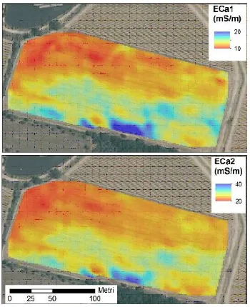
The proximal sensing with EM38-Mk2 provided very similar maps of ECa1 (0-75
cm) and ECa2 (0-150 cm), showing lower ECa values (10-20 mS/m) in the northern
part of the field (profiles 1 and 2) and higher values (25-40 mS/m) in the southern part (profiles 3 and 4) (Fig.2).
Gamma-ray total counts (TC) showed a general homogeneous pattern (260-280 Bq/kg), with the only exception of a small area in the southern part, represented of red area (220-230 Bq/kg) observable in Fig.2 and delimited by the area of profile 4. The maps of radionuclides (40K, 232Th, 238U) showed the same low values in the area of profile 4, but high noise in the rest of the field. For this reason, we decided to remove these layers from the clustering calculation.
and Bucelli, 2008), we decided to map 4 STUs by supervised classification. Therefore, the map obtained by the supervised classification (Fig. 3) was very similar to that obtained by k-means clustering (Fig.1).
Figure 2
Maps of total count of gamma-ray (TC), and apparent electrical conductivity at
about 0-75 cm (ECa1) and 0-150 cm
(ECa2).
////
Table 1.Soil profiles description
P Horizon
De p th S an d
Clay Sil
t Coar se fr agm e n ts CaC O3 tot .
BD(1) Ksat(2) SOC(3) Ntot(4) CEC(5) Kexch(6)
cm % g∙cm-3 mm∙h-1 g∙kg-1 meq∙100g-1 mg∙kg-1
1
Ap1 25 35.6 34.6 29.8 18 2.3 1.40
6.0
10.3 1.18 14.9 125.1
Ap2 45 36.7 34.5 28.8 23 1.2 1.55 10.3 1.17 15.3 129.1
Bw1 90 31.8 41.3 26.9 30 2.3 n.d. 4.6 0.78 15.5 70.4
Bw2 110 38.7 32.5 28.8 10 3.2 n.d. 3.0 0.56 14.2 66.5
2
Ap1 30 40.6 29.7 29.7 10 0.6 1.34
17.0
12.0 1.22 14.5 109.5
Ap2/Bw1 90 48.5 27.4 24.1 10 2.6 1.43 8.3 0.88 14.5 70.4
Bw2 120 26.5 37.7 35.8 2 3.2 1.66 3.8 0.54 14.1 62.6
3
Ap1 30 36.2 35.7 28.1 8 0.7 1.50
0.6
10.3 1.12 15.5 113.4
Ap2/Bw 90 39.9 33.8 26.3 15 0.6 1.36 8.5 0.94 16.4 117.3
Bw/Btg 110 24.5 46.9 28.6 2 0.2 1.55 2.6 0.4 16.4 62.6
Btg 140 23.8 49.2 27.0 15 0.1 n.d. 1.3 0.4 16.0 50.8
4
Ap 15 19.5 41 39.5 10 38.5 1.62
<0.1
6.8 0.86 11.5 105.6
Bkg1 40 21.9 40.1 38.0 10 41.6 1.66 5.2 0.79 11.1 89.9
Bkg2 100 12.5 39.1 48.4 10 48.7 1.68 1.2 0.28 8.6 78.2
(1) Bulk density; (2) Saturated Hydraulic permeability, measured by Guelph permeameter; (3) Soil organic carbon; (4) Total
[image:4.482.246.425.107.224.2]If STU1 and 2 were similar, and they could be grouped to simplify the vineyard management, STU3 and 4 had important peculiarities, which have to be taken in account during vineyard planning.
[image:5.482.57.426.181.316.2]The peculiarities of STU4 was probably due to the proximity of the calcareous hill. Although the actual surface of the field was approximately flat, the STU4 represent an edge of the calcareous hill, which was levelled in the past. Indeed, the soil of STU showed all the feature of truncated soil, which were shallow A and B horizons (40 cm), very poor organic matter and very high calcium carbonate contents, starting from the surface (Fig.3, P4).
Figure 3. Pictures of the studied soil profiles.
This high content of calcium carbonate and the high frequency of waterlogging in the soil of STU4, classified as Calcaric Stagnosol (IUSS Working Group WRB, 2014), testifies sub-surface water fluxes from calcareous hill, which tend to transport a great amount of Ca+ ions in water solution, partly released as pedogenic calcium carbonates in this area. STU3 showed slow water drainage and waterlogging features probably due to poor structure and compaction in depth (90-100 cm).
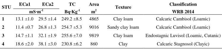
Table 2.Summary of the mean values of proximal sensing data of each STU and the soil features of the associated soil profile.
STU ECa1 ECa2 TC Area Texture Classification
mS∙m-1 Bq∙Kg-1
m2 WRB 2014
1 13.1 ±1.0 29.5 ±1.4 249.2 ±8.5 4865 Clay loam Calcaric Cambisol (Loamic)
2 11.4 ±0.7 26.8 ±1.3 254.7 ±5.3 9016 Sandy clay loam Calcaric Cambisol (Loamic)
3 14.7 ±1.1 32.1 ±1.9 255.6 ±7.0 9819 Clay loam Endostagnic Luvisol (Loamic, Cutanic)
4 18.6 ±2.0 38.1 ±3.0 230.8 ±6.2 860 Clay Calcaric Stagnosol (Clayic)
ECa1 and ECa2: apparent electrical conductivity measured by EM38-MK2 at 0-75 and 0-150 cm, respectively; TC: gamma-ray total count measured by “The Mole”.
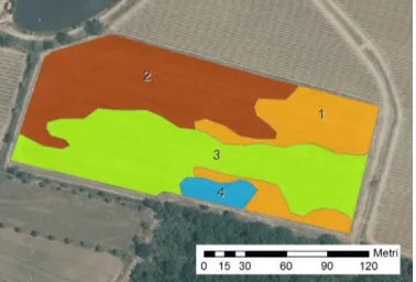
[image:5.482.54.428.478.561.2]Figure 4
Final STUs, obtained after Supervised classification and simple filter to simplify the geometry.
The detailed mapping of STUs (Fig.4), allowed to base the vineyard planning on soil spatial variability. In particular, the farmer made a deep trench between calcareous hill and the field, to interrupt and regulate the sub-surface water fluxes and made an artificial drainage in STU3 (depth 70-90 cm). On the basis of this investigation, the farmer decided to use for the STU1, 2 and 3 a rootstock more resistant to carbonates and plant chlorosis like 140Ru, instead of the previously selected 110R rootstock.
Acknowledgments: The authors want to thank the winery “Petra” for the financial
support of this research work and for their will to plan new vineyards according to a scientific and site-specific approach. The authors want to thank the reviewer for the fruitful and accurate comments.
References
BONFANTE A., AGRILLO A., ALBRIZIO R., BASILE A., BUONOMO R., DE MASCELLIS R., GAMBUTI A., GIORIO P., GUIDA G., LANGELLA G., MANNA P., MINIERI L., MOIO L., SIANI T., TERRIBILE F. (2015) Functional homogeneous zones (fHZs) in viticultural zoning procedure: an Italian case study on Aglianico vine. Soil, 1(1): 427.
COSTANTINI E.A.C, BUCELLI P. (2008). Suolo, vite ed altre colture di qualità: l’introduzione e la pratica dei concetti “terroir” e “zonazione”. Italian Journal of Agronomy, 3:23-33.
DOOLITTLE J., PETERSEN M., WHEELER T. (2001). Comparison of two electromagnetic induction tools in salinity appraisals. Journal of Soil and Water Conservation, 56(3):257-262.
GEBBERS R., LÜCK E., DABAS M. (2009). Comparing of instruments for geoelectrical soil mapping at the field scale. Near Surface Geophys. 7(3):179–190.
IUSS WORKING GROUP WRB (2014) World Reference Base for soil resource 2014. World Soil Resources Reports n. 106, FAO, Rome (Italy).
LANYON D.M., CASS A., HANSEN D. (2004) The effect of soil properties on vine performance. CSIRO Land and Water Technical Report n.34/04.
McNEIL J. D. (1990) Geonics EM38 ground conductivity meter: EM38 operating manual. Geonics Limited, Ontario, Canada.
ORTUANI B., CHIARADIA E. A., PRIORI S., L'ABATE G., CANONE D., COMUNIAN A., GIUDICI M., MELE M., FACCHI A. (2016) Mapping Soil Water Capacity Through EMI Survey to Delineate Site-Specific Management Units Within an Irrigated Field. Soil Science, 181(6):252-263.
PRIORI S., FANTAPPIÈ M., MAGINI S., COSTANTINI E. A. C. (2013) Using the ARP-03 for high-resolution mapping of calcic horizons. International Agrophysics, 27(3):313-321.
PRIORI S., BIANCONI N., COSTANTINI E. A. (2014). Can γ-radiometrics predict soil textural data and stoniness in different parent materials? A comparison of two machine-learning methods. Geoderma, 226:354-364.
REYNOLDS W. D., ELRICK D. E. (1985) In situ measurement of field-saturated hydraulic conductivity, sorptivity, and the α-parameter using the Guelph permeameter. Soil Science, 140(4):292-302.
SAXTON, K. E., RAWLS, W. J. (2006) Soil water characteristic estimates by texture and organic matter for hydrologic solutions. Soil Science Society of America Journal, 70(5): 1569-1578.
SCHOENEBERGER P. J. (2002) Field Book for Describing and Sampling Soils: Version 2.0 (No. 631.47). National Soil Survey Center, Natural Resources Conservation Service. STEPHENS D., DIESING M. (2014) A comparison of supervised classification methods for the prediction of substrate type using multibeam acoustic and legacy grain-size data. PloS one, 9(4):e93950.