ADAPTIVE SIMULATION MODEL CONFIGURATION
by
Randall Gray, B.A. (Flinders University of South Australia)
Submitted in fulfilment of the requirements for the Degree of Doctor of Philosophy
Discipline of Mathematics University of Tasmania
I declare that this thesis contains no material which has been ac-cepted for a degree or diploma by the University or any other in-stitution, except by way of background information and duly ac-knowledged in the thesis, and, to the best of my knowledge and belief, no material previously published or written by another per-son, except where due acknowledgement is made in the text of the thesis; nor does the thesis contain any material that infringes copy-right.
Dr Simon Wotherspoon is listed as a contributor to the papers in-cluded as Chapters 2 and 3, his contribution to each of the papers was predominantly as a sounding board and a source of encour-agement. His direct input into the papers was primarily concerned with the structure of the paper and its ordering rather than its con-tent.
Signed:
ThepublishersofthepaperscomprisingChapters2and3holdthe copyrightforthosechapters,andaccesstothematerialshouldbe soughtfromtherespectivejournals.Theremainingnon-published contentof thethesis maybe made available forloan andlimited copyingandcommunicationinaccordancewiththeCopyrightAct 1968
Signed:
Statement of Co-Authorship
School of Natural Sciences, Mathematics Randall Gray (Candidate) University of Tasmania Dr Simon Wotherspoon (Supervisor)
Author details and their roles:
Paper 1,Increasing model efficiency by dynamically changing model representations
Located in Chapter 2.
The candidate, Randall Gray, was the primary author and was responsi-ble for the conception, design, implementation, preparation of graphics, analysis of the work described in the paper, and writing the paper it-self. Dr. Wotherspoon contributed guidance as to how to improve the presentation of the work and make it accessible to a broader audience before submission, and provided advice on addressing the concerns of the reviewers.
Paper 2,Adaptive submodel selection in hybrid models
Located in Chapter 3.
The candidate conceived the ring-like structure used in paper, estab-lished the algebraic properties of the structure and proved the relevant theorems. The candidate also designed the thought model described in the paper, prepared the tables and graphics and was wrote the paper. Again, Dr. Wotherspoon contributed by acting as an informal reviewer, highlighting those parts of the paper that were inadequately explained or difficult to follow, and after acceptance by providing advice on ad-dressing reviewers’ comments.
Signed:
Dr Simon Wotherspoon Supervisor
Institute for Marine and Antarctic Studies
Date:
Signed:
Prof Mark Hunt Head of School
School of Natural Sciences
ABSTRACT
Models of complex systems may be improved in fidelity, efficiency or both by allowing the way they represent component parts to change as the state of the model and its components move through their state-spaces.
A simple model demonstrates that representation changes for a population en-countering contaminants may perform better than either conventional form. Here, there was a substantial decrease in runtime relative to a purely i-state configuration (individual-based) model, with comparable fidelity, while the purelyp-state (population-based) version exhibited error arising from the `blurring” of contaminant contact through the distributed population. This example demon-strates the utility of model representations maintain important state data across representations so that previous representations can be recovered with mini-mal error.
Triggers for changing representations of components is addressed in a paper exploring a possible set of dynamics associated with a simple, hypothetical model of a seven component ecosystem. The components of the system are described asi-state configuration models or as p-state models, and a mecha-nism for determining when to change representations is outlined.
ACKNOWLEDGEMENTS
TABLE OF CONTENTS
TABLE OF CONTENTS 2
LIST OF TABLES 6
LIST OF FIGURES 7
1 INTRODUCTION 9
1.1 Motivation . . . 12
1.1.1 Implications of the effects of behaviour, vulnerability and change . . . 13
1.1.2 Implications of the effects of social dysfunction . . . 15
1.2 Comparable work . . . 15
1.3 Structure . . . 18
1.4 Scales . . . 20
1.5 Outline . . . 22
2 INCREASING MODEL EFFICIENCY BY DYNAMICALLY CHANG-ING MODEL REPRESENTATIONS 24 2.1 Prologue to the paper . . . 24
2.2 Introduction . . . 26
2.3 Overview: anODDmodel description . . . 29
2.3.1 Purpose . . . 29
2.3.2 State variables and scales . . . 30
2.3.3 Process overview and scheduling . . . 31
2.4 Design concepts . . . 31
2.5 Details . . . 32
2.5.1 Initialisation . . . 32
TABLE OF CONTENTS 3
2.5.2 Input . . . 32
2.5.3 Submodels . . . 33
2.6 Results . . . 35
2.6.1 Contaminant load correspondence between representa-tions . . . 36
2.6.2 Contaminant load variability . . . 36
2.6.3 Sensitivity to the shape of the plume . . . 37
2.6.4 Run-time . . . 38
2.7 Discussion . . . 39
2.7.1 State spaces . . . 39
2.7.2 Heuristics . . . 40
2.7.3 Transitions . . . 40
2.7.4 Errors . . . 41
2.8 Conclusion . . . 42
2.9 Epilogue to the paper . . . 43
3 ADAPTIVE SUBMODEL SELECTION IN HYBRID MODELS 44 3.1 Prologue to the paper . . . 44
3.2 Introduction . . . 46
3.3 Model organization . . . 48
3.3.1 Implications of changing configurations . . . 49
3.3.2 Systematically adjusting the model configuration . . . 51
3.4 The example model . . . 53
3.4.1 IBPlants . . . 56
3.4.2 IBAnimals . . . 56
3.4.3 The monitor and model dynamics . . . 58
3.5 Discussion . . . 64
3.6 Conclusion . . . 66
3.7 Appendix . . . 67
3.7.1 Mathematical definitions . . . 67
3.8 Epilogue to the paper . . . 70
TABLE OF CONTENTS 4
4.2 Conventions and preliminary definitions . . . 72
4.3 Scalar Multiplication and addition . . . 75
4.3.1 Scalar multiplication and some convenience functions . . 75
4.3.2 Addition . . . 75
4.4 Properties of a vector space . . . 76
4.5 Seminorms, norms and metrics . . . 81
4.5.1 Tand its classwise seminorm . . . 82
4.6 Element multiplication in ˇTand establishing the properties sim-ilar to those of a ring . . . 84
4.7 Discussion . . . 87
5 THEORY AND AN EXAMPLE IMPLEMENTATION 88 5.1 Formative design considerations . . . 89
5.2 Principles . . . 90
5.2.1 Interactions . . . 90
5.2.2 Time . . . 91
5.2.3 Changing representation . . . 91
5.2.4 Assessment and adaptation . . . 92
5.3 Framework and Example implementation . . . 92
5.3.1 Scheme . . . 93
5.3.2 SCLOS– aSchemeimplementation ofCLOS . . . 96
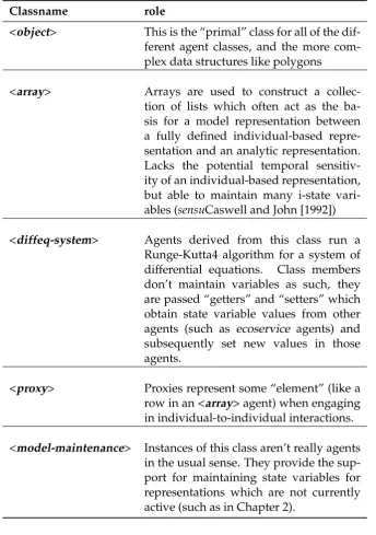
5.3.3 Class structure . . . 96
5.3.4 Parameterisation . . . 103
5.3.5 Model initialisation . . . 106
5.3.6 Methods, model bodies and closures . . . 106
5.4 Execution and Control flow . . . 107
5.5 Interaction with the kernel and other agents . . . 108
5.5.1 Calls to the kernel . . . 108
5.5.2 Spatial queries . . . 109
5.6 Introspection agents: loggers and monitors . . . 110
5.6.1 Generating output files – loggers . . . 110
5.6.2 Changing representations . . . 111
5.6.3 Comparison of states . . . 114
TABLE OF CONTENTS 5
5.7.1 Distributed models . . . 116 5.7.2 Cross-representation interactions . . . 116 5.8 Observations . . . 120
6 Conclusion 123
6.1 Into the future . . . 127
A TYPESETTING CONVENTIONS 130
B SNAPSHOTS OFREMODELRUN 131
C SUPPLEMENTARY MATERIAL 135
LIST OF TABLES
2.1 Parameters associated with individual movement . . . 33 2.2 Maxima and Means . . . 36 2.3 Deviations amongst the model runs with respect to a given mean 37 2.4 Circular plume results . . . 38 2.5 Elliptical plume results . . . 38
5.1 Fundamental classes in theRemodelframeworkframework-classes.scm 97 5.2 More fundamental classes –framework-classes.scm. . . 98 5.3 Introspection classes inRemodel–introspection-classes.scm . . . 100 5.4 Basic individual-based representations –framework-classes.scm. . 101 5.5 Non-spatial environments elements –landscape-classes.scm . . . . 102 5.6 Spatial environments –landscape-classes.scm . . . 103 5.7 Symbols . . . 117
A.1 Printing styles . . . 130
LIST OF FIGURES
2.1 Snapshots of individuals’ locations at 28 day intervals superim-posed on the migratory path. The plume’s contact domain is marked by a grey ellipse near the position of individuals at day 28, with the track of a single individual approaching it. The do-main of a population is is circumscribed around the individuals at day 196 for comparison. . . 30
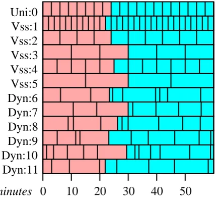
3.1 Time scheduling strategies. Red boxes represent time steps that have already passed, blue boxes represents scheduled time steps that have not yet been run. “Uni:” and “Vss:” submodels are members of a uniform or variable speed splitting submodels and require uniform time steps, and “Dyn:” submodels have adaptive time steps. . . 50 3.2 The model domain is divided into nine cells. AnSD agent is
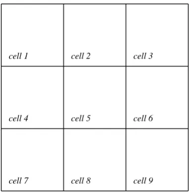
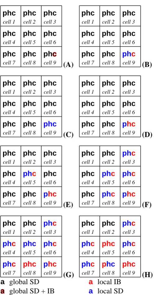
associated with each of these cells and with the domain as a whole. AnyIBagents which are created during the simulation will be associated with one cell at any given time. . . 53 3.3 The color of thep,handcindicate an agent’s current
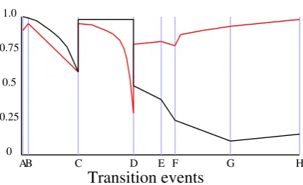
representa-tion within a cell at various points in the descriprepresenta-tion of a simula-tion. In each, a black symbol indicates that the biomass of plants (p), herbivores (h) or carnivores (c) is modeled with the global SDagent, a blue symbol indicates that the biomass is modeled with a cell’sSDagent, and red indicates that anIBmodel is be-ing used. Symbols composed of two colors indicate that more than one representation is currently controlling portions of the relevant biomass. . . 61 3.4 Normalized indexes of execution speed (black) and fidelity (red)
the against configuration changes through time associated with Figure 3.3 . . . 62
B.1 Snapshots of tree-cover locations at day 0. The herbivore is not visible, because it hasn’t moved yet. . . 132 B.2 Snapshots of tree-cover locations at day 25. The herbivore is
LIST OF FIGURES 8
C
HAPTER
1
Introduction
Modellers of complex systems are often faced with the task of coupling com-ponents which may operate at quite different scales with the goal of creating a useful tool for study these systems. This thesis puts forward the argument that better1 models may be built if we allow the representation of component parts of a model to change according to
their states,
the nature of their interactions with other components, the needs and states of the other components
and
the state of the model as a whole.
The majority of the discussion will be couched in the context of biological or environmental systems, but it is not limited to this area: the context was cho-sen for its familiarity, its generality, and because models of ecosystems often incorporate significant environmental, physical and biochemical submodels such as inATLSS [DeAngelis et al., 1998], Atlantis[Fulton et al., 2011b], and
InVitro[Gray et al., 2014].
A mechanism for deciding how close complex mixtures of agents are to nom-inative “good” or “bad” configurations is necessary, so a mathematical struc-ture is developed which can be used to encode information about the model’s constituents and their relationships. This structure is a normed vector-space, and can be used to assess the relative utility of a configuration by comparison with a corpus of configurations which are either preferred or deprecated. The assessment and conversion of components from one form to another is a potentially burdensome process; to alleviate this, and make the approach more useful, a framework for constructing models,Remodel, is developed in Chapter 5. It treats models as being composed of niches which are analogous to environmental niches. Much as an environmental niche may be occupied by members of a number of different species, a niche in the framework may 1Here,bettercan mean ‘less error, faster, more consistent with field dataor whatever the model in question is configured to optimise. This objective may also change through the life of the simulation.
10
be populated by instances of different types of agents. In an environment, the succession of occupants in a niche is driven by the state of the system, and organisms which are morefit for the state replace those which perform less well. The same sort of principle may be applied inRemodel. While it can be used in much the same way as other modelling frameworks, such asNetLogo
[Wilensky, 1999] orSwarm[Minar et al., 1996], the framework provides sup-port for modellers to indicate what conditions are favourable for different rep-resentations which fill the niches in the models and to automatically replace agents which are ill-suited to their context with more appropriate representa-tions when the need arises. The framework is explored using thethought-model of Chapter 3 as a notional equivalent of an artist’s mannequin.
Such a strategy has a number of potential benefits:
– we can make many simple representations, submodels, for a niche (sensuGray et al. [2006] and Gray et al. [2014]) in the model, each of which deals well with a particular part of the submodel’s domain;
– the comparative simplicity of these representations effectively reduces the number of potential code paths within a model at any given moment, since representations do not have to cope with edge cases, they merely indicate that they are entering a marginal or inappropriate domain;
– we can use analytic representations which are more efficient at represent-ing large numbers of entities;
– we can use individual-based representations which capture the fine-scale dynamics that dominate when we are dealing with discrete events or low numbers of entities;
– we can choose representations that make the best use of available data within the model, or can ask for better representations in the ensemble;
– it is simple to incorporate code to track information about representation changes, relative execution speed, and cumulative error into the mod-elling system;
– we may include agents that identify the emergence of perverse dynamics within the system;
and
– we can decouple the production of the results from processes which sim-ulate the systems and subsystems being modelled.
11
simple to address the questions “How do we deal with situations where the as-sumptions that underpin our representation no longer hold?” and “How do we man-age the execution of submodels which simulate systems or entities with multi-modal behaviour?”
Consider this example: rather than a single representation for the population of a coastal city, we may have a number of different submodels with different levels of aggregation and different temporal or spatial scales. In a simulation of a cyclone season, we may start with a simple single age-histogram representa-tion. As a tropical storm builds we may disaggregate the histogram, appropri-ately distributing the population to finer age-histograms associated with local-ities throughout the region. As it approaches the coastline, the essentially static representations which lie in areas likely to suffer damage are converted into agents instances of running submodels which represent households. Shortly before the cyclone reaches the point where damage occurs, we may resolve the representation further, instantiating emergency response agents and con-verting households agents to individuals at risk. In the aftermath, aggregation may occur in regions where there are no acute effects, but other parts of the system may remain finely resolved.
In this example, we change the representations to deal with both of the ques-tions above. We initially assumed that for most of the purposes of the simu-lation, our population could be treated as relatively homogeneous, and may have kept aggregate information about population distribution, wealth and demographic characteristics, but as the storm hits, the simulation needs to change the state of a portion of the population (those with damaged prop-erty, for example), and we have to refine our representation. Similarly, the behaviours following the storm are modally different: those who live in pro-tected areas are mostly free to carry on with essentially the same normal rep-resentation, but those who are living in damaged areas must engage in quite different activities, and may have quite a different exposure to risks.
Adaptive approaches commonly occur in techniques for numerical approxi-mation (regression, root finding, and parameter estiapproxi-mation for example), nu-merical solutions for systems of differential equations, feature detection and recognition, control systems and route planning. Often these approaches in-volve adjusting the size of the domain considered (subdivisions or step size), or the rates associated with a process. In the case of route planning, sets of routes may be marked as impassable as data becomes available, triggering a reassessment of the set of possible routes. More broadly, domain adaptation describes a general approach where a model or system adjusts itself to the data it works with one of the canonical examples is a Bayesian spam filter which includes a users assessment of whether email is spam or not in its subsequent assessments. A common trait these adaptive techniques share is that the algo-rithm which processes the data remains essentially the same.
1.1. MOTIVATION 12
individual-based modelling is now a common approach. Individual-based or super-individual-based models are not a panacea. These types of models may become costly as the number of individuals or the interactions between in-dividuals or super-inin-dividuals grows, and small discrepancies between the behaviour or parameterisation of the modelled entities and their real counter-parts may produce large discrepancies at the population level. Many of the parameters that may influence the life-history of organisms at an individual level are difficult or impossible to estimate in situ, and so the effects of individ-uals modelled behaviours or processes may not scale well when incorporated in larger systems.
Discrete changes in the behaviour of a system, or part of a system, are com-monplace. The scales of systems that exhibit switching behaviour range from a molecular level, such as the behaviour of freezing liquids, through the in-termediate scales to the changing climate. Evidence for a broad recognition that systems dynamics can (and do) switch rapidly from one ostensibly stable mode to another is that the discussion of tipping points has increased dramat-ically in the last decade [Bhatanacharoen et al., 2011].
1.1
Motivation
There are a number of situations where the nature of a system changes to such a degree that the fundamental dynamics we might normally use to simulate the system are inappropriate. In models of animal populations, it may be that the number of individuals may have climbed to the point that inaccuracies in individual-based models begin to dominate the dynamics of the system, or that the number of individuals has declined to the point that an analytic rep-resentation is unable to capture the dynamics of a small population. We ought to be able to reduce our model error by choosing appropriate representations for the conditions, and to limit the propagation of error into components that depend on other submodels. Such partitioning also makes error estimation more straightforward.
We can also find examples systems that are subject to serious perturbation arising from small deviations from their “nominal” condition. Traffic flow, for example, can be dramatically constrained by obstructions (sudden or other-wise) on the roadway with consequences that spread quite a long way from the source. Another potential source of perturbation which may have signifi-cant effects is a change in behaviour in some subset of components of the sys-tem. In the context of biological systems, this is particularly so if the change impinges on the viability of individuals or their ability to reproduce.
1.1. MOTIVATION 13
(systems dynamics, discrete event simulations, and individual-based models, for example). These toolkits have a broad user base and include support for essential facilities such as generating graphic output or interaction with GIS systems: their focus is on making robust tools available to modellers across a range of research domains. They have, however, no explicit support for mod-els where the representations of entities may actually change their form. As mentioned above, we are comfortable with real-world systems where things undergo dramatic changes: water freezes, some insects go from egg to nymph and nymph to adult as part of their life-cycle: it seems a natural conclusion that simulations of these things may benefit from an analogous process.
1.1.1 Implications of the effects of behaviour, vulnerability and change
alter-1.1. MOTIVATION 14
native representations for affected and unaffected portions of the populations are indicated.
When an altered behaviour or biological efficiency is associated with the spread or reproduction of organisms, the scope for destructive feedback is increased, and the dynamics can diverge rapidly from representations that are adequate for an unperturbed system. The effects of Toxoplasma gondiion rats [Berdoy et al., 2000] is an ideal example: rats inoculated with the parasite (usually by contact with infected cat faeces) lose their innate fear of cats. The positive rein-forcement on the spread of T. gondii afforded by this leads to greater potential for the pathogen to infect more cats, and hence, more rats. The behaviour of the rats is clearly not consistent with the behaviour one would usually encode in a model of a rat population. In a similar paper, van Dobben [1952] observes that roaches (Rutilus spp) infected with Lingua intestinalis were three to five times more numerous in cormorant catches than in the roach population of the IJsselmeer2(as estimated from commercial catches), suggesting that some-thing in the fishs behaviour makes them more susceptible to capture. In these cases, special steps would be needed to to model the populations, either ana-lytically or in simulation, to avoid underestimating both the mortality of the prey species and the presence of the pathogens in the definitive host.
Dobson [1988] contains a brief summary of literature that addresses parasitic infection which alters the hosts behaviour to benefit the parasites reproduc-tion. Particularly useful are the analyses of the consequence of the interac-tion for both the definitive host that parasites breed in, and intermediate hosts which are used to reach the definitive host3. In a broader study, Poulin [1994] assesses the effect on host behaviour in a number of host-parasite pairings, and found that the parasites had a significant effect on the behaviour of their hosts.
These papers concerning the effect of parasites on host behaviour suggest that the influence of parasitism on populations may be greater than we might ex-pect. Lafferty et al. [2006] argue that parasitism is the dominant mode of trophic interaction, and that their role is significantly absent in the literature. The implication is that for trophic models of any sort, there needs to be a body of robust techniques to manage the transition of parts of a population from uninfected to infected and some means of dealing with them which preserves their properties appropriately. While Dobson provides an analytic example, it is clearly limited by the requirement of sufficient population sizes to make the analytic representation tenable its application in situations where local extinction is a possible outcome may not be tenable.
It is also possible for populations which are afflicted by behaviour modifying 2A large lake in the Netherlands.
3The author also presents several systems of differential equations which describe the
1.2. COMPARABLE WORK 15
parasites toalsobe vectors for contaminants which affect their predators. Man-aging the resulting cascade of influence may have particular relevance when considering strategies for the management of vulnerable species. An appropri-ate expression of behaviour influences reproduction and predation dynamics and is thus essential in simulation models.
When a significant portion of a population is infected with these types of par-asites, we can no longer treat the population as homogeneous, and the rates for reproduction and mortality vary significantly between infected and unin-fected sub-populations. In this scenario, there it is a reasonable assertion that infected portions of the population should be treated separately from the un-infected population.
1.1.2 Implications of the effects of social dysfunction
The situation is more complex when there are endogenous reasons for fun-damental changes in an organisms basic dynamics. Unnatural situations can induce radical, even pathological, changes in behaviour. Social animal popula-tions may behave in quite strange ways when their population density grows too large, there are stressors which are alien to them, or the populations so-cial profile is disrupted. A seminal (and grim) example of this is described in Calhoun [1973]. Calhoun recounts an experiment in which mice are con-fined in a domain where all their physical needs were met, all possible sources of mortality apart from senescence and death by injury were excluded, and there was no possibility of emigration. Social and behavioural disintegration began to manifest in the third generation (day 315), and the population went into terminal decline after 560 days, and for all practical purposes the social organisation had collapsed utterly.
Calhoun discounted the population density as the cause of the social disinte-gration, rather attributing the collapse to the inability of young adults to en-gage in normal roles due to high competition for thesocial nicheswhich were filled by older, dominant mice. The behavioural changes attending the so-cial collapse did not revert to more normal behaviour when population levels dropped (past 560 days). This type of response to social conditions may be pertinent for other species, and it has clear implications for simulation mod-els of social animals. Behaviour associated with social settings is, almost by definition, context dependent. This paper illustrates that, at least in social an-imals, dramatic changes in models of behaviour may be required, and that those changes may be dependent on thesocial contextrather than the physical environment. The social connections maintained may be as important to the survival of an individual as access to shelter or food in some circumstances.
1.2
Comparable work
1.2. COMPARABLE WORK 16
both in terms of basic biological activity and in their interactions with other el-ements in the simulated domain. This comes at a cost. Tracking the fine scale modal properties more closely requires decision or selection strategies which ensure that the models behave in ways that are appropriate for the context. Many individual-based models incorporate environmental characteristics that influence the behaviour of the individuals simulated. Botkin et al. [1972a,b] and DeAngelis [1978] are important early examples: Botkin et al. dealt with systems that modelled the effect of spatially explicit environmental conditions on simulated trees (rather than stands or coupes) in a mixed species popula-tion in North America; in the case of DeAngelis, the model was used to explore the distribution of fish (modelled as individuals) in a speculative body of wa-ter with a known distributions of temperature and food availability. Both of these models simulated the dynamics resulting from the physical conditions real plants and animals might encounter and they reflected observed patterns to a striking degree. Many processes occur over short time spans, small do-mains or both, and these models provided a means of simulating these pro-cesses over appropriate scales. These models were successful because they they increased the fidelity of their representation, and were able to generate results that were more intuitively accessible to non-experts because they re-flected observable processes. They also represent the scientific realisation that traditional population-level models relying on a significant degree of homo-geneity may not be appropriate in heterogeneous environments. What they demonstrate is that the form a model should take ought to be sensitive to the conditions and dynamics which prevail in the system being simulated.
Hu and Edwards [2005] describe a model of crayfish is constructed in the DEVS framework using component submodels which competitively assess various behaviours and select one or more of these behaviours based on thresh-old values as an appropriate response to the environment and the state of the crayfish agent. An essentially similar strategy for behaviour selection was used in in Lyne et al. [1994b] for unimodal behaviour selection and in Gray et al. [2006, 2014] for restricted multi-modal behaviours. These works base the execution (or not) of particular branches of code model on assessments com-prised of their own state and that of their environment. In this way, they bear a similarity to the model selection described in subsequent chapters; while this approach to nuanced simulation is only focussed on the behaviours evinced by the agents, it foreshadows modal representation dictated by dynamic as-sessment.
1.2. COMPARABLE WORK 17
Bobashev et al. [2007] describes a model of epidemic simulation in which the representations of populations or portions of populations are decided based on the number of infected individuals relative to a nominated trigger value. This model demonstrates that there is a demonstrable advantage to changing rep-resentation in terms of computational efficiency and the fidelity of the model. The published model in Chapter 2 is similar: when individuals with contami-nant loads in Chapter 2 leave the region where contamination is possible, they are subsumed back into the population and their data is incorporated so that the individual contaminant profiles are maintained and subject to depuration. Both of these models are an improvement on traditional individual-based and equation-based methods: local conditions are able to affect the outcome for individuals, and the computational load of individual-based simulation is re-duced when appropriate. The aim is to preserve the fidelity of the individual-based data, while benefiting from the speed and mathematical tractability of an analytic or numerical model. In both of these models, the triggers for change are fairly basic – numbers of infected individuals or presence within the zone of potential contamination.
Much like Bobashev et al. and the model in Chapter 2, the model described in Wallentin and Neuwirth [2017] is a hybrid predator-prey model that exhibits model switching. The model simulates a lake with fish and plankton, switch-ing between equation-based lake-wide representations and agent-based rep-resentations for fish at either a sub-region level or as individuals, and plank-ton were represented either by a global model or by local cellular-automata. Again, changes in representation were by transitions past nominated trigger values. These swapping strategies are ideal for models which focus on a lim-ited set of simple dynamics, but whether this is adequate for more complex ensembles is unclear.
The pedestrian detection and tracking system of Zhang et al. [2016] selects the algorithms and parameters to be used in the analysis of segments of data based on the nature of the data it is given. Their approach has qualitative similarities to the approach suggested in this work, since the whole method of evaluation changes based on its input, rather than adjusting the scales or domains. They accomplish this by training the selection system off-line on known data. Their selection system corresponds to a member of particular class inRemodelcalled amonitor. Themonitoragents are fundamental to the automatic control of the mix of representations in the running model: they interrogate sets of agents and are able to initiate changes in representation. Monitorsare able to make use of a corpus of sets containingknown-goodandknown-badconfigurations: a situation which corresponds closely with Zhang et al.. Themonitorsalso have the ability to adjust this corpus according to the dynamics at play within the simulation and so may be reactive as well as adaptive.
1.3. STRUCTURE 18
remain4, it provides a road-map with signposts to aid newcomers to the do-main.
There is clearly a growing set of models which demonstrate that adaptive hy-brid models are both feasible and worthwhile. However, the mechanisms be-hind changes in representation in the literature are both simple and largely based on local state information. The exploration of the issues associated with the maintenance of state information across transitions is also largely absent. There is no systematic support for transitions in response to the needs of other components of the systems, or mechanisms that enable systematic collection of data regarding the performance of the model. Most importantly, there are no fundamental code-bases from which model development can proceed. The work that follows addresses these deficits and constructs a more comprehen-sive framework that is able to support models with complex conditions related to representational transitions, and to support the maintenance of state data across transitions.
1.3
Structure
Models of complex systems usually incorporate alternative code paths or ex-pressions in a component to deal with situations where there are fundamen-tally different dynamics or properties by testing for these conditions at each potential fork in the code. In many cases, this sort of control flow may decide between a number of paths, but the selection protocol and consequent paths are all hard-coded within the model. Such a structure can engender a com-plicated network of potential execution paths through the model. In contrast, the approach discussed in this thesis addresses this problem by constructing the models as an ensemble of agents which can cede their role to another rep-resentation which is more suitable when the need arises. A resident popula-tion might be represented by a singlepopulationagent, a set ofindividual-based agents,super-individualagents or by some mixture of these representations. Models of complex systems usually incorporate alternative code paths or ex-pressions in a component to deal with situations where there are fundamen-tally different dynamics or properties by testing for these conditions at each potential fork in the code. In many cases, this sort of control flow may decide between a number of paths, but the selection protocol and consequent paths are all hard-coded within the model. Such a structure can engender a compli-cated network of potential execution paths through the model. In contrast, the approach discussed in this thesis addresses this problem by constructing the models as an ensemble of agents which can cede their role to another repre-sentation which is more suitable when the need arises. A resident population might be represented by a single population agent, a set of individual-based agents, super-individual agents or by some mixture of these representations. The decision to change the representation of a submodel occupying a niche
4Such as might be posed by situations analogous to gape limited predation between
1.3. STRUCTURE 19
in the model should be based on the state of the system, the capabilities (or incapability) of the agents in the system and the objectives of the modeller in configuring a model, we might prioritise speed over accuracy for a real-time simulation, a computer game or a combat training simulator, and for a scien-tific extrapolation of the state of a harbour for each of a number of develop-ment scenarios, we might choose accuracy over speed.
Representing the state of the model, either as a whole or of its constituent parts, is not simple: not only may the submodel mix in the niches of the model vary through time, but the dependences of submodels on other components and niches may change as the state of the model changes. A model which con-tains a whale spotting tourism venture may follow the activities of whales at particular times of the year, but be utterly indifferent to the whales at times when there is little likelihood of their presence in an accessible location. Simi-larly, the association of entities represented by a population-based model may need to be maintained if the population disaggregates into agents based on super-individuals (small cohorts) or agents representing individuals.
The interplay of factors like these make a simple vector-based encoding mech-anism for the states of a model and its components awkward, thus we turn to a metric space whose elements are trees with a finite number of weighted, la-belled nodes. This simplifies the comparison of possible ways to fill the niches in the model for a given global state, and makes available any algorithms (par-ticularly useful are clustering) which depend only on the properties of a metric space.
The decision to change representations can be made by an agent that recog-nises that it is unable to continue in the conditions in which it finds itself (akin to the code-path decisions in more traditional models), or by a similar assertion from some higher agency (a monitor in the discussion which follows) which assesses states more broadly. In the case of an agent determining that it needs to change, such as a penguin moving from the nestling submodel to the juve-nile submodel, this can be effected directly, though the more general (and in this case, burdensome) strategy would for a monitor to flag the desired state change and then act on it when appropriate.
The models explored in this work bear a resemblance to a multitasking operat-ing system, but, unlike an operatoperat-ing system, the models kernel must maintain temporal ordering of agents’ start times within the agent queue, and this order must be strictly non-decreasing. Interactions between agents are largely me-diated by the kernel and new agents may be created or removed with relative ease. Choosing this as an organisational template means that there are many patterns to serve as templates for further development.
1.4. SCALES 20
1.4
Scales
The natural time step or spatial scales of a model may change if one or more of its constituent submodels changes its representation. This seems like an ob-vious statement, but many models are structured with quite carefully chosen time steps and spatial scales, and they may behave poorly when these scales are changed. Examples of this, such as Lyne et al. [1994a], Xu et al. [2001], Zhang and Montgomery [1994], model systems where the appropriate time-step is intimately linked to the temporal scale of the system being studied. Component submodels of the models in Lyne et al. [1994a] (and of Gray et al. [2006] and Gray et al. [2014]) were tested during development for the effect of length of an individual’s time-step on the component’s dynamics. The re-sults of the first of these models prompted the use floating point variables for time in subsequent models, and time-steps with intervals determined by a continuous function based on the individual’s conditions, activity and inter-actions. In Lyne et al. [1994a], the smallest time-step was conditioned by the interval where a simulated organism’s contaminant uptake was reasonably stable: steps which were too long either over-estimated or under-estimated potential uptake, and steps which were too short suffered both from compu-tational inefficiency, and accumulated error in the movement of the modelled individuals. Xu et al. [2001] found that simulations of mesoscale convective systems were sensitive to the size of the time-step, even though the model re-mained numerically stable. They found that the predicted precipitation could vary by as much as 50% when the time-step was reduced from 225s to 50s, and attributed the change to the dependence on the time-step size of the calcula-tions associated with the horizontal diffusion. Zhang and Montgomery [1994] found that grid-size for digital elevation maps in hydrological models had a significant effect on the results of simulations.
Fulton et al. [2004b] examines the effect of spatial resolution of the dynamics of marine populations using two models of a large bay. The domain is parti-tioned into regions (boxes) filling the domain both vertically and horizontally. Two particularly important observations are made: coarse spatial resolutions in the model lead to a simplification of the trophic web relative to fine-scale simulations, and the spatial resolution must reflect the dynamics of scale of the dominant gradients and processes in the system. This sentiment is also reflected by a conclusion in a paper produced by the FAO,
At the end of this process the necessary components will need to be represented at the appropriate scales in prototype or final model(s). It is important to reemphasise here that there is no one single right model. All models have problems and it is best (where possible) to use a range of models that can address the question in different ways.
1.4. SCALES 21
Generally, representations of individual organisms are likely to require much smaller temporal and spatial scales than representations at a population level, so a model which seeks to accommodate both possibilities must be able to ac-commodate the scales that are important at that point in the simulation. For temporal scales this means providing the infrastructure to ‘buffer’ the activ-ity of agents with longer time-steps, and to ensure that – as far as possible – the temporal discrepancy amongst the agents is minimised. Agents with long steps will necessarily often be ahead or behind agents with shorter time-steps. Changing spatial resolution seems relatively straightforward, but the errors that accompany spatial misregistration or integration over an inappro-priately interpolated domain can become significant.
Changes in temporal scale can be more problematic, however. Time influences causality in a way that space does not. Deciding how to manage the flow of time in an ecological simulation model is one of the first decisions in its de-sign. Many ecological models have been constructed as a large set of arrays containing state variables which are inspected and updated in the body of an event loop (or many loops). Some models achieve temporal optimisation by dividing the arrays into various groups of fast-stepping and slower-stepping variables, only dealing with the necessary parts of the system at each time step (variable speed splittingas in Walters et al. [2000], for example). Gray et al. [2006] and Gray et al. [2014] allow agents to dynamically determine their own time step based on their state – time steps may be truncated, or changed for their next turn in response to their situation. There is a trade-off in this: with a variable speed splitting approach, we can calculate all values based on a temporally coherent set of data, and update them all in one pass; in contrast, the dynamic time stepping approach means that each interaction is essentially conducted in isolation, and the consequences of a set of interactions may be dependent on the order in which the interactions occurs. Both variable speed splitting and dynamic time step selection are flexible enough to support rep-resentational changes for entities, but the greatest advantage comes from con-structing the submodels to be robust with respect to arbitrary time steps over a reasonable domain. If a model is consistently run with time steps which are too long or too short, the model or system needs to be able to initiate a change to a more appropriate representation.
Inappropriate or incommensurate time steps can pose a real problem: while the interactions between submodels with short time steps and submodels with long time steps may be managed, at least to some degree, by accumulating changes to the slower model and applying them during the slower model’s time step, this is not an ideal solution. One of the major risks this approach poses is a of distortion of resource availability which is dependent on the order in which agents are executed. This sort of error can artificially inflate or deplete apparent resources in a seemingly random fashion, and render the results of the simulation useless.
1.5. OUTLINE 22
which may occur as a result of interactions large changes may call for small time steps.
1.5
Outline
The paper5which forms the body of Chapter 2 develops a model of organisms that periodically move through a region subject to plumes of contaminant. The model is capable of modelling the organisms either with a population-based representation or with an individual-based representation. This model is run in three configurations: purely population based, purely individual-based and as a hybrid where the individual-based representation is used when it is pos-sible for any of the population represented to come into contact with the con-taminant, and with the population-based elsewhere. An essential notion that was treated lightly in this paper is developed much more fully, namely that for a model to allow an oscillation between representations, additional data must be passed between them, maintained and possibly adjusted in order to preserve consistency across transitions.
The purpose of the model is to demonstrate the feasibility and utility of main-taining the contaminant loads (more generallystate data) while running in a different representation and to compare both the execution speed of the simu-lations and the fidelity of the simulation with respect to the contaminant loads of the simulated population. The study found that the trials which alternated representations based on the proximity to the contaminated region was con-sistent with the individual-based trials, but performed with a computational speed of the same order as the population-based trials.
Chapter 3 was published6 in a special issue ofFrontiers in Environmental Sci-ence. It considers a small three species ecosystem and explores the properties needed for a more complex evaluation of possible model-swapping configu-rations of a running model, and develops a thought-model as a platform for discussion. To support the dynamic assessment and selection of model con-figurations, the paper introduces a metric space based on a tree structure. The metric space allows us to calculate distances between configurations and to re-duce our potential search spaces by identifying clusters of representations that are largely similar in their constitution.
Chapter 4 presents a modified version of the appendix included in Chapter 3. The modifications make the structures easier to manipulate, and code to perform mathematical operations on these objects forms the basis for the se-lection process in the realised modelling framework and the example model discussed in Chapter 5.
There are many consequences which arise from the premise that the agent or set of agents which represent part of a simulation may change and that the synthesis of what they represented may be represented by a different set of
5https://doi.org/10.1016/j.envsoft.2011.08.012
1.5. OUTLINE 23
agents. The discussion in Chapter 5 seeks to highlight and explain these con-sequences and the response to them, referring both to theRemodelframework and to the example model that was described in Chapter 3 and built within the framework. Currently the framework is functional, but still requires a more fully developed set of transition mechanisms, basic classes (for things other than animals, trees and monitors), and is lacking in a broad set of ex-ample models. Many of the functional niches inRemodelhave more than one possible representation, and these representations can change in response to their own state, the states of other agents, or even the requirements of other agents. Where possible, the options for model selection differ in an important and fundamental way: they span the range from individual-based represen-tations, through intermediates which represent a number of individuals, to conceptually continuous models. These changes are, in some sense, analogous to the transition from the set of integers to the set of real numbers. A model which demonstrated the utility of adaptive representations without changing the “cardinality” of the system would have been much simpler, but it would have missed some of the most important parts of the problem.
— — —
The corpus of code in the framework is a little under 28,500 lines ofScheme
code and is freely available at
http://github.com/snarkypenguin
The interpreter/compiler used in this work isGambitdeveloped by Marc Fee-ley. It has a thriving community, excellent support and integrates well withC
andC++, and is available from the GitHub repository
https://github.com/gambit
While the model does not requireSLIBby Aubrey Jaffer,SLIBprovide a broad range of useful functions.SLIBis available at
http://people.csail.mit.edu/jaffer/SLIB.html
———–
Dr Simon Wotherspoon was credited in the papers which comprise Chapters 2 and Chapter 3, in acknowledgement of his salient advice to me on how to ap-proach the task of writing papers both for journals and for a broader audience, and how to avoid getting distracted by the little stuff.
The corpus of code in Remodel is a little under 28500 lines ofSchemecode and is freely available athttp://github.com/snarkypenguin/Remodel.git
The interpreter/compiler used in this work isGambitdeveloped by Marc Fee-ley. It has a thriving community, excellent support and integrates well withC
andC++, and is available from the GitHub repositoryhttps://github.com/gambit
While neither the framework nor the model requiresSLIB by Aubrey Jaffer,
SLIBprovides a broad range of useful functions.
C
HAPTER
2
Increasing model efficiency by
dynamically changing model
representations
2.1
Prologue to the paper
The body of this chapter is a (verbatim) paper published in the refereed jour-nalEnvironmental Modelling and Software(Gray and Wotherspoon [2012]). The model discussed in this chapter is built using an older, much simpler body of code than the framework that is explored in Chapter 3. While the primary purpose of the paper is indicated by its title, a significant contribution is its development of the basic mechanisms for changing representations.
The source-code can be obtained from
https://github.com/snarkypenguin/Model-Efficiency.git.
The paper explores a model of marine organisms that periodically migrate through an intermittent plume of some contaminant. The uptake and depura-tion of the contaminants in the organisms are modelled, and the paper com-pares the results and the run-time for the system in three forms in order to establish how useful using model switching may be in terms of run-time and fidelity. The three configurations tested are
• a purely analytic representation of the migrating population – In this configuration a population whose relative locations follow a Gaussian distribution is moved around the migratory circle, and the uptake of con-taminant is calculated using a Runge-Kutta4 algorithm
• a purely individual-based model – Individuals move through the con-taminant zone, integrating their contact with the plume and generating an uptake level appropriately
2.1. PROLOGUE TO THE PAPER 25
• either a population (as described), a set of individuals (also as described), or as a mix with part of the cohort represented as individuals within the risk zone, and the balance represented as a population – Here, individ-uals are generated (and removed from the population) as the popula-tion disk encroaches on the contaminant zone. As individuals leave the contact zone, they are subsumed by the population and their individual contaminant level is decayed appropriately.
The analytic submodel is the simplest of the representations, consisting largely of a value (or vector) which records the contaminant load, and the number of individuals which are represented. A single instance of the analytic submodel is present in both the purely analytic model and in the switching model. The individual-based model incorporates a number of state variables, such as ve-locity, contaminant load and the instantiated agents are independent of the analytic representation.
In order to avoid confounding the results, the contaminant is inert since in-cluding toxicity effects would have the potential to alter both the number of entities modelled and their behaviour (such as movement rates); since slower individuals would take longer to move through contaminated regions, their likelihood of contact would be higher. The scenario in the model would be substantially similar to simulating the uptake of isotopes associated with par-ticular geographic locations.
Given the very predictable dynamics of the modelled entities, the inclusion of multiple contaminants or multiple sources, such as in Gray et al. [2006, 2014], seemed unlikely to do anything surprising.1
1incorporated mortality or morbidity associated with contact, the mortality strategy used in
2.2. INTRODUCTION 26
Increasing model efficiency by dynamically changing
model representations
Randall Gray2
CSIRO Division of Marine and Atmospheric Research
Simon Wotherspoon University of Tasmania
Abstract
There are a number of strategies to deal with modelling large complex systems such as large marine ecosystems. These systems are often com-prised of many submodels, each contributing to the overall trajectory of the system. The balance between the acceptable modelling error and the run-time often dictates the form of these submodels. There may be scope to improve the position of this balance point in both regards by structuring models so that submodels may change their algorithmic rep-resentation and state space in response to their local state and the state of the model as a whole.
This paper uses an example system consisting of a single population of animals which periodically encounters a diffuse contaminant in a lo-calised region as an example of such a system, and discusses the key issues that arise from the approach.
2.2
Introduction
There is a body of literature stretching back several decades which discusses individual-based modelling as a useful alternative to classical models. Early examples modelled forest canopy dynamics, notably JABOWA and its deriva-tives Botkin et al. [1972b,a]. The number of significant papers and books has steadily increased since the 1980s. These works describe the use of individual-based models across a broad range of systems, and the relative strengths and weaknesses of the approach (such as Huston et al. [1988], DeAngelis and Gross [1992] and Grimm and Railsback [2005]). Classical models exploring popula-tions and ecological systems are usually associated with modelling the dy-namics of large groups and arguably appeared at the end of the eighteenth century with Malthus’sAn Essay on the Principle of Population(1798). The
2.2. INTRODUCTION 27
properties of these models are well understood and their state variables usu-ally correspond to measurable quantities. Often, they are much faster than individual-based counterparts, and the analysis of model error may be much more straightforward. Classical and individual-based approaches represent the ends of a spectrum of aggregation in time, space and membership. Rep-resentations lying between these extrema, such as described by Scheffer et al. [1995], capitalise on the process-fidelity of an individual-based representation and gain some of the computational efficiency of a more aggregated classical approach, but an adaptive exploitation of the strengths of different represen-tations is possible and worth exploring.
Ecosystem models are becoming broader in scope (Rose et al. [2010], DeAn-gelis and Gross [1992], Harvey et al. [2003]?Fulton et al. [2004a], Gray et al. [2006], Gray et al. [2014]) and include more species with richer environments. The environmental response to climate change has also made anthropogenic pressure an important feature in many of these models. As this trend grows it seems less likely that a single model drawn from any particular region of this spectrum will be able to address all members and processes equally well. Simulation models often embed their subject in an “environment” comprised of primary data and other models and these components may occupy many places in the spectrum of representations. The model’s actual implementation may be anything from a set of distinct models which are coupled together but retain their independence, to a corpus of code with the submodels so inte-grated that there is no real distinction between one “model” and the next. The dynamics associated with biological and ecological systems can depend on the distributions and states of individuals in ways which are not amenable to equation-based modelling. The individual-based models described in Farolfi et al. [2010], and de Almeida et al. [2010] deal with systems of this sort. Ver-sions of these models could be embedded in a common simulation environ-ment in order to address more complex problems which span traditional do-main boundaries, and such a model could address broader questions, such as how mosquito control strategies may best adapt to evolving agricultural practices and watershed conditions. Thiele and Grimm [2010] describes an extension to NetLogo which allows modellers to incorporate calls toR func-tions to aid in configuring the model to meet desirable mathematical condi-tions, to provide ongoing analysis, and to display the model’s state through its run. This interface betweenRandNetLogo could be extended to support incorporating mathematical decision models written inRinto the model’s de-cision tree. The fusion of these three elements would form a system capable of simulating possible trajectories for the management of watersheds and hu-man health in ways which would not be possible with a traditional monolithic modelling approach.
2.2. INTRODUCTION 28
This paper explores the technique of changing the representation of a com-ponent of a model based on its location in its state-space. Modellers already do this to some degree: time-steps or spatial resolutions are changed, partic-ular code paths may be by-passed to avoid pointless work, or additional cal-culations might be performed to reduce the error when the state is changing rapidly. These optimisations are largely optimisations of theencoding of the model or submodels, rather than an actual change in representation.
Vincenot et al. [2011] make a clear case for considering what the authors term “hybrid-models.” They present four reference cases which they use to describe ways in which equation-based models and individual-based models might be coupled to increase their utility. Their categories of hybrid-models are: individual-based models interacting with a single system dynamics model, system dynamics models embedded in based models, individual-based models interacting with a number of system dynamics models, and models in which the representation swaps between individual-based and an equation-based form. They argue that a hybrid approach may provide a means of increasing the speed and accuracy of our models; Gray et al. [2006], and? have demonstrated that large models of ecosystems can be modelled this way. Vincenot et al. note that they found relatively few models which use both individual-based and equation-based submodels, and they present no exist-ing models representexist-ing their fourth reference case. This final case, where models swap from equation-based to individual-based, is briefly described in general terms and is clearly intended to encompass models like the model of this paper.
This “mutating” or “switching” approach to the problem of managing com-plex simulations was developed using the experience from making several large scale human-ecosystem interaction models (Lyne et al.; Gray et al. [2006]; and a current, larger study of Ningaloo coastal region (work in progress)). In each of these studies a significant component of the model focused on sim-ulating the interaction between organisms and contaminant plumes, though there is nothing that inherently limits the techniques to these sorts of stud-ies. Lyne et al. assessed the potential of contaminants originating in indus-trial waste percolating through the food chain into commercially exploited fish stocks. Gray et al. developed a regional model to assess management strate-gies for human activity which interacts with the biological systems along the Northwest Shelf of Australia.
2.3. OVERVIEW: ANODDMODEL DESCRIPTION 29
with contamination. Monte discusses a method of coupling the equations which govern contaminant dispersion with the equations for population dy-namics and migration. The technique depends on the equations of the location and the dispersion of members of a population satisfying an independence condition with respect to time and location which must hold. He states that the class of systems where the “movement of animals, the death and birthrates of individuals in x [location] at instant t [time] depend on previously occu-pied positions” is not generally amenable to the approach and suggests that repeated simulations of many individuals is an appropriate way of dealing with this situation.
It is unnecessary to run a complex model and carry the burden of maintain-ing its state when a simple model may perform better. If representations are switched appropriately, there is potential for improvements in run-time and accuracy. We need to consider four basic questions to do this:
1. What data need to persist across representations?
2. When should a model change representation?
3. How is the initial state for a new representation constructed?
4. How should the error associated with the loss of state information be managed?
The answer to these questions is specific to the set of submodels in question. Before expending resources and effort on a large scale model there needs to be a demonstration that the notion is worth pursuing, and some indication of how it might be accomplished. The aim of this paper is to provide this demon-stration rather than to develop a comprehensive body of techniques support-ing the approach. Many systems may benefit from similar techniques; obvious candidates are models of marginal populations, and the population dynamics of animals with behaviour where short periods of time have a significant influ-ence on population levels (Wolff [1994] and Elderd et al. [2008], for example).
2.3
Overview: an
ODD
model description
TheODDprotocol [Grimm et al., 2006] is used to describe the example model. We discuss the issues associated with making such a system, strategies and the reasons behind them in the Discussion section.
2.3.1 Purpose
2.3. OVERVIEW: ANODDMODEL DESCRIPTION 30
shares a number of features with plausible models and the analysis and de-velopment of the mutating model should be a reasonable template for other systems.
[image:35.595.239.343.283.378.2]The model simulates organisms moving along a simple migratory path which intersects a region containing a field of fluctuating contamination (see Fig-ure 2.3.1). This model exhibits fundamental attributes of larger studies of pol-lutant/ecosystem interactions (Lyne et al. and Gray et al.) and, while it is not intended to accurately represent any particular system, it might loosely corre-spond to some body of water influenced by contaminant loads associated with terrestrial runoff resulting from intense rainfalls.
Figure 2.1: Snapshots of individuals’ locations at 28 day intervals superim-posed on the migratory path. The plume’s contact domain is marked by a grey ellipse near the position of individuals at day 28, with the track of a sin-gle individual approaching it. The domain of a population is is circumscribed around the individuals at day 196 for comparison.
The test models are composed of one or more submodels which run within a simple time-sharing system. Each submodel runs for a nominated period of time and passes control to the next submodel, very much like tasks running in many modern computer operating systems. In amutatingconfiguration, a trial will have different models take turns representing components of the system. The population-based and individual-based submodels have been kept as sim-ilar as practicable in order to minimise the sources of divergence.
2.3.2 State variables and scales
encom-2.4. DESIGN CONCEPTS 31
passes both the area influenced by the contaminant source and the annual mi-gratory path of the organisms. The plume can be viewed as a forcing function in the model and it has a maximum footprint area of approximately 43km2 which may be circular or elliptical and is centered on a point of the migra-tory circle. Both the elliptic and circular variants of the plume have the same area, and their intensities are adjusted so that the integral of the contaminant concentration over the region is the same.
The individual-based representation maintains a contaminant load associated with contact with the plume, a location, a direction and the next time at which it is scheduled to run. The population-based representation treats the group as homogeneous with respect to all state variables other than the contaminant load, and maintains only a record of its next time-to-run and an indication of contaminant load in the population. In the straight population-based rep-resentation, this is a single value, but in the mutating system the submodel maintains a list of contaminant loads which correspond to the non-zero loads of individuals. The plume model is deterministic with respect to time and location and maintains no state variables.
2.3.3 Process overview and scheduling
Simulations were run with 90 minute time-steps for a period representing twelve years. At each time-step, each instance of a submodel is rostered in a priority queue sorted on the “time-to-run” state variable, and when it comes to the top of the queue it executes.
Populations operate in a straightforward way: their path is deterministic, ex-posure to contaminants is calculated, and the resulting values are fed through the uptake-depuration equation. Individuals calculate their path (a segment of a directed random walk which follows the path of migration) and contact for the time-step and an apply the uptake-depuration equation. At the end of a time-step in non-mutating configurations, data is accumulated for output and each submodel reinserts itself in the priority queue. Otherwise, a heuristic is used to choose an appropriate representation for the niche in next time-step and that is inserted into the queue. Randomisation within a time-step is un-necessary, since the individual’s or the population’s contaminant updates are resolved for the contaminant contact across their time-step and are not depen-dent on the state of any other agents.
2.4
Design concepts
2.5. DETAILS 32
associated with triggering a change from a population-based representation to individuals and a corresponding heuristic which indicates when an individ-ual should join (or become) a population. The actindivid-ual mechanism which turns a population into individuals or its converse is not necessarily a property of those models. Since the objective is to examine the impact of changing model representation in a fairly narrow situation, no attempt is made to optimise the submodels in the “non-contact” areas which constitute most of the model do-main.
2.5
Details
2.5.1 Initialisation
Individuals and populations initially begin with no contaminant load, and in-dividuals are positioned according to the two-dimensional normal distribu-tion which characterises the populadistribu-tion’s assumed distribudistribu-tion. When a pop-ulation mutates into an appropriate set of individuals, the individuals are posi-tioned in the same fashion (centered on the centre of the population) with their corresponding contaminant loads either taken from the list of non-zero con-taminant loads maintained by the population or initialised to be zero should the population’s list fall short.
2.5.2 Input
Several characteristic features of the model are determined by the time and lo-cation represented. The contaminant intensity (and hence extent) at any point, r, relative to the centroid of the plume,mplume, at a time,t, by the equation
I(t,r)=1
2(1+cos(2πt/p))exp(−ψϕ(r,mplume))
where p is the period of 34 days, ψ = 0.05 is a decay exponent. We take
ϕ to be a distance function, either ϕ(a,b) = ∣a−b∣, for a circular plume, or
ϕ(a,b)=
√
(a−b)⋅(√2,√1/2), for an elliptical plume. The effective radius of the circular plume in the model is about 3.7% of the circular migratory path of the populations and individuals. The intensity of the elliptical plume is ad-justed by scalar multiplication so that the integral ofIfor the two plumes over their domain is the same.
2.5. DETAILS 33
2.5.3 Submodels
Individual-based representation
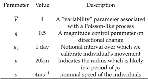
[image:38.595.145.436.289.444.2]Individuals follow a directed random walk around the migratory circle de-scribed in the previous section. At each time-step the stride the individual takes is calculated according to its proximity to the “target” on the migratory path. There are a number of parameters associated with the movement of the individuals presented in Table 2.1.
Table 2.1: Parameters associated with individual movement
Parameter Value Description
V 4 A “variability” parameter associated with a Poisson-like process q 0.5 A magnitude control parameter on
directional change
µδ 1 day Notional interval over which we
calibrate individual’s movement
µ 20km Indicates the radius which is likely in a period ofµδ
s 4ms−1 nominal speed of the individuals
If we takeδto be the length of the current time step, andv to be a realisation of an event in a Poisson-like process with a mean ofV, we can take
Q=[1−exp(v¯
Vlog(1−q))]
to be a “variation” scalar which we use to evaluate an effective radial speed,
νs=RRRRRRRRRR
RR−1+ √
1+4sQ2δ ¯ VRRRRRRRRRRRR/2Q
2.
Large values of Q correspond to long stretches of time without a change in direction, so we include Q in the calculation of α, the partial change in the individual’s direction vector, by setting it to α = πrnd(−Q,Q). We can take their effective displacement over the 90 minute interval to be determined by a weighted sum of the normalised vector which joins them to their “target” location on the migratory path and a direction vector of length νs which is deflected byα.
Population-based representation