Inverse space-dependent force problems for the wave equation

This is a repository copy of Inverse space-dependent force problems for the wave equation.

White Rose Research Online URL for this paper: http://eprints.whiterose.ac.uk/97757/

Version: Accepted Version

Article:

Lesnic, D, Hussein, SO and Johansson, BT (2016) Inverse space-dependent force

problems for the wave equation. Journal of Computational and Applied Mathematics, 306. pp. 10-39. ISSN 0377-0427

https://doi.org/10.1016/j.cam.2016.03.034

(c) 2016, Elsevier B.V. This manuscript version is made available under the CC-BY-NC-ND 4.0 license http://creativecommons.org/licenses/by-nc-nd/4.0/

[email protected] https://eprints.whiterose.ac.uk/

Reuse

Unless indicated otherwise, fulltext items are protected by copyright with all rights reserved. The copyright exception in section 29 of the Copyright, Designs and Patents Act 1988 allows the making of a single copy solely for the purpose of non-commercial research or private study within the limits of fair dealing. The publisher or other rights-holder may allow further reproduction and re-use of this version - refer to the White Rose Research Online record for this item. Where records identify the publisher as the copyright holder, users can verify any specific terms of use on the publisher’s website.

Takedown

If you consider content in White Rose Research Online to be in breach of UK law, please notify us by

Inverse space-dependent force problem for the wave

equation

D. Lesnic1_{, S.O. Hussein}1 _{and B.T. Johansson}2

1_{Department of Applied Mathematics, University of Leeds, Leeds LS2 9JT, UK} 2_{Aston University, School of Mathematics, Birmingham B4 7ET, UK}

E-mails: [email protected], [email protected], [email protected]

Abstract.

act-ing on a vibratact-ing structure from measured final or time-average displacement observation is thoroughly investigated. Several issues related to the existence and uniqueness of solution of the linear but ill-posed inverse problems are highlighted. After that, in order to capture the solution a variational formulation is proposed and the gradient of the least-squares functional that is minimized is rigorously and explicitly derived. Numerical results obtained using the Landweber method and the conjugate gradient method are presented and discussed illus-trating the convergence of the iterative procedures for exact input data. Furthermore, for noisy data the semi-convergence phenomenon appears, as expected, and stability is restored by stopping the iterations according to the discrepancy principle criterion once the residual becomes close to the amount of noise. The present investigation will be significant to re-searchers concerned with wave propagation and control of vibrating structures.

Keywords:

Conju-gate gradient method; Wave equation.

1

Introduction

We consider the problem of force identification from measured data for the hyperbolic wave equation. This inverse formulation is significant to modelling several practical applications related to unknown force loads and control. Because part of the cause of the physical phenomenon is unknown one has to compensate for this lack of information by measuring an appropriate part of the effect. What quantity to measure is the delicate choice/constraint when formulating inverse problems, but a proper formulation would be able to ensure that the unknown force can be uniquely retrieved from the proposed additional measurements.

Prior to this study, the reconstruction of a space-dependent force in the wave equa-tion from Cauchy data measurements of both displacement and its normal derivative on the boundary has been attempted in [3, 10, 11]. This inverse formulation is, as expected, improperly posed because the unknown output force f(x) depends on x in the domain Ω, whilst the known input data, say u and ∂nu, depend on (x, t)on the boundary ∂Ω_×(0, T). Although the uniqueness of solution still holds, [6, 14, 18], it seems more natural to mea-sure instead information about the displacement u(x, t) for x _∈ Ω and time t = T, or the time-averaged displacement RT

0 u(x, t)dt for x ∈ Ω. This way, the output-input mapping

employs a weak solution approach for a quite general inverse problem with a highly non-unique solution, and to [17] which nicely introduces a quasi-nonlinearity in the governing wave equation to resolve the non-uniqueness of solution. The other inverse problem generated by the measurement of the time-averaged displacement RT

0 u(x, t)dt which we investigate in

our study is new. Essentially, the same inverse problem with unknown spacewise dependent right-hand side source in the governing equation arises also for the parabolic heat equation in the thermal field, see [8, 13].

The plan of the paper is as follows. Section 2 introduces the inverse problem formulations, whilst Sections 3 and 4 highlight several issues related to the existence, uniqueness and stability of solution of the direct and inverse problems, respectively. Section 5 presents the variational formulations of the inverse problems under investigation and derives explicitly the expressions for the gradients of the least-squares functionals which are minimized. Section 6 describes the iterative Landweber method accommodated and applied in order to obtain regularized stable solutions, whilst Section 7 illustrates and discusses extensive numerical results in both one and two dimensions, for the recovery of both smooth and non-smooth force functions. Furthermore, the conjugate gradient method (CGM) is also described and employed for one of the examples. A numerical extension to two-dimensions is presented in Section 8 and finally, conclusions are presented in Section 9.

2

Problem formulation

Assume that we have a medium, denoted by Ω, occupying a bounded sufficiently smooth domain in Rn_{, where n≥1. The boundary of Ω is denoted by∂Ω, and we define the} space-time cylinder QT = Ω_×(0, T), where T >0. We wish to find the displacement u(x, t) and the force f(x) in the hyperbolic wave equation

utt_{− L}u=f(x)g(x, t) +χ(x, t) =:F(x, t) in QT, (1)

where g and χ are given functions, and, in general, for a homogeneous medium we have

L=_∇2 _{the Laplacian operator. For inhomogeneous media, we can haveLu=c}2_(x)∇2_{u, or}

∇.(K(x)_∇u), where K and care given positive material properties, [4]. Equation (1) has to be solved subject to prescribed initial conditions

u(x,0) =ϕ(x) x_∈Ω, (2)

ut(x,0) =ψ(x) x_∈Ω, (3)

prescribed homogenous Dirichlet boundary conditions,

u(x, t) = 0, (x, t)_∈∂Ω_×(0, T), (4)

and the additional final displacement measurement

u(x, T) = uT(x), x_∈Ω, (5)

or, the time-average displacement measurement

Z T

0

ω(t)u(x, t)dt =UT(x), x_∈Ω, (6)

3

Direct problem

Well-posedness of the direct problem (1)-(4) when f is given, is provided in Section 7 of [2] for example. Suitable space are: F _∈L2_{(QT), ϕ∈H}1

0(Ω)withLϕ∈L2(Ω), andψ ∈H01(Ω),

then u_∈C2_{(0, T;L}2_{(Ω)) with u(t)∈H}1

0(Ω) and Lu(t)∈L2(Ω) for t∈[0, T].

One can also study weak solutions u _∈ L2_{(0, T;H}1

0(Ω)) with ut ∈ L2(0, T;L2(Ω)) and

utt _∈L2_{(0, T;H}−1_{(Ω)). Such a weak solution exists and is unique provided thatϕ ∈H}1 0(Ω),

ψ _∈ L2_{(Ω) and F ∈ L}2_{(QT). Note that, as usual, this implies u ∈ C([0, T];L}2_{(Ω)) and}

ut _∈ C([0, T];H−1_{(Ω)), which, in particular, yield that the restrictions at t = 0 of the}

solution and its derivative make sense. Moreover, we have the estimate

max 0≤t≤T

||u(., t)_||H1

0(Ω)+||ut(., t)||L 2

(Ω)

+_||utt_||L2

(0,T;H−1(Ω))

≤C_||F_||L2_(0,T;L2_(Ω))+||ϕ|| H1

0(Ω)+||ψ||L 2_(Ω)

, (7)

for some positive constant C.

Similar considerations can be done for the formally adjoint backward hyperbolic problem to (1)-(4),

vtt_{− L}∗v =G(x, t), (x, t)_∈QT, (8)

v(x, T) =ζ(x), vt(x, T) = ξ(x), x_∈Ω, (9)

v(x, t) = 0, (x, t)_∈∂Ω_×(0, T), (10)

where _L∗ _{is the adjoint ofL.}

Furthermore, we have, using integration by parts, the following Green-type formula:

Z

Ω

(ut(x, T)ζ(x)₋ψ(x)v(x,0))dx₋

Z

Ω

(u(x, T)ξ(x)₋ϕ(x)vt(x,0))dx

= Z T

0 Z

Ω

F(x, t)v(x, t)dxdt₋

Z T

0 Z

Ω

G(x, t)u(x, t)dxdt. (11)

3.1

Abstract setting formulation

It is possible to formulate the direct problem (1)-(4) in a more general abstract setting, as described in Chapter 8 of [16], by considering the problem

u′′=_Lu(t) +F(t), t_∈[0, T], (12)

u(0) =ϕ, u′(0) =ψ, (13)

where_Lis a closed linear operator with a dense domain of definitionD(_L)on a Hilbert space X. We assume that _L generates a strongly continuous cosine function C(t) = cos(√_−Lt), such that equation (12) is hyperbolic. In the case of a self-adjoint operator, the previous assumption is equivalent to say that _L is semi-bounded from above, [16, p.525]. According to [16, p.538], if

ψ _∈E :=_{u_∈X_|C(t)u_∈C1_{(R)}, (15)}

F _∈C1([0, T];X)_⊕C([0, T];D(_L)), (16)

then the direct problem (12) and (13) has a unique solution in the class of functions

u_∈C2([0, T];X)_∩C([0, T];D(_L)). (17)

Furthermore, one can represent explicitly this solution as

u(t) =C(t)ϕ+S(t)ψ+ Z t

0

S(t₋s)F(s)ds, (18)

where S(t) =Rt

0C(s)ds = 1 √

−Lsin(

√

−Lt) is the associated sine function.

4

Inverse problem

Consider first, for simplicity, the one-dimensional case, i.e. n= 1, and takeΩ = (0, L), where L > 0 represents the length of a vibrating string. Let us also take χ(x, t) = 0, g(x, t) = 1

and _L = ∂2_/∂x2_{. Then, in [3] it was remarked that the inverse force problem (1)-(5) has}

a unique solution if and only if T /L /_∈ Q, i.e. T /L is an irrational number. This follows immediately from the separation of variables, whereas forϕ =ψ = 0 andg = 1 the solution of the inverse problem

utt₋uxx =f(x), (x, t)_∈(0, L)_×(0, T), (19)

u(x,0) =ut(x,0) = 0, x_∈(0, L), (20)

u(0, t) =u(L, t) = 0, t_∈(0, T), (21)

u(x, T) = 0, x_∈(0, L), (22)

is given by

u(x, t) =

√

2

π2 ∞ X

k=1

ck k2

1₋cos

kπt L

sin

kπx L

, (23)

f(x) = ∞ X

k=1

cksin

kπx L

, (24)

where

ck =

√

2

L

Z L 0

f(x) sin

kπx L

Now, in order to impose (22) we apply (23) at t=T to obtain

0 =

√

2

π2 ∞ X

k=1

ck k2

1₋cos

kπT L

sin

kπx L

, x_∈(0, L). (26)

One can easily observe thatck= 0 for allk _≥1, and hence from (23) and (24),u=f = 0, if and only if T /L /_∈Q. Moreover, this condition cannot be removed even if one additionally prescribeut(x, T), as it can be easily seen by differentiating (23) with respect tot. However, if we consider the additional time-average displacement measurement (6) (with say ω = 1) instead of (5), by integrating (23) with respect tot and make it zero, we obtain

0 =

√

2

π2 ∞ X

k=1

ck k2

T ₋ L

kπsin

kπT L

sin

kπx L

, x_∈(0, L). (27)

Since kπT

L >sin kπT

L

for all k _∈ N∗, we then obtain that ck = 0 for all k _∈ N∗ and hence, from (23) and (24), that u =f = 0. Thus, the inverse problem (19)-(21) together with the integral condition

Z T 0

u(x, t)dt = 0, x_∈(0, L), (28)

has only the trivial solution, which in turn implies that the solution of the inverse problem given by equations (19)-(21) and the time-average displacement measurement

Z T 0

u(x, t)dt=UT(x), x_∈(0, L), (29)

is unique, with no restriction on the ratio T /Lbeing irrational number or not. Of course, in the case of an arbitrary integrable weight function ω(t) in (6), the necessary and sufficient condition for uniqueness becomes

Z T

0

ω(t)

1₋cos

kπt L

dt₆= 0, _∀ k_∈N∗. (30)

4.1

Abstract setting formulation of inverse problems

Returning to the abstract setting of subsection 3.1 and viz. Section 2, we consider the inverse problem of determining the displacement u and the force f satisfying

u′′ =_Lu(t) +g(t)f, t_∈[0, T], (31)

subject to the initial conditions (13) and the additional measurement

u(T) =uT (32)

or

Z T

0

First, the following theorem gives the unique solvability of the inverse problem (13), (31) and (32).

Theorem 1.

In the abstract settings of subsection 3.1, let _Lbe a self-adjoint and semi-bounded from above operator in the Hilbert space X and assume that the input data is admissible, i.e.

ϕ_∈D(_L), ψ _∈E, g _∈C1([0, T];X), χ_∈C1([0, T];X)_⊕C([0, T];D(_L)), (34)

and

uT _∈D(_L). (35)

Then the inverse problem (13), (31) and (32) has a unique solution u _∈ C2_{([0, T];X)∩}

C([0, T];D(_L)), f _∈ X if, see Corollary 8.2.7 of [16], g is non-negative and strictly in-creasing, as a function of t _∈ [0, T], or if, see Corollary 8.2.8 of [16], g _≡ 1 and 1 _∈/ Z, where

Z :=_{cos(√₋λ T) _| λ_∈Σ(_L)_\{0_}}, (36)

and Σ(_L) denotes the spectrum of the operator _L.

In the above, the valueg(s)is identified with the operator of multiplication by the number g(s) in the spaceX.

Remark that in the previous one-dimensional setting of the inverse problem (19)-(22) the condition that1_∈/ Z recasts as1₋cos(√₋λ T)₆= 0, whereλ =₋n2_π2_/L2 _{forn ∈N}∗_{, which}

is equivalent to say that T /L /_∈Q.

We note that for _L =_∇2_{, Ω∈C}1_{, ϕ, ψ, u}

T ∈C1(Ω) satisfying compatibility conditions and g _∈ C1_{(QT) satisfying g(x, t) >0, gt(x, t) > 0, ∀(x, t) ∈ Q}

T, the existence of solution, i.e. the solvability of the inverse problem (1)-(5) was also established in [1] in the classes of functions f _∈L2_(Ω),u∈L2_{(0, T;H}1_(Ω)),u

tt ∈L2(QT)and ∇2u∈L2(QT).

Second, for the inverse problem (13), (31) and (33) we also have the existence and unique-ness of solution as given by the following theorem.

Theorem 2.

In the abstract setting of Theorem 1 and with the same input admissible data (34), and

ω = 1, UT _∈D(_L), (37)

the inverse problem (13),(31)and (33)has a unique solutionu_∈C2_{([0, T];X)∩C([0, T];D(L)),}

f _∈X, if 0_6≡g is non-negative, as a function of t _∈[0, T].

Proof. On applying (6) to (18) results in

Φ(_L)f =UT −S(T)ϕ−

(1₋C(T))

−L ψ−

Z T 0

Z t 0

S(t₋s)χ(s)dsdt, (38)

where

Φ(_L) = Z T

0 Z t

0

g(s)S(t₋s)dsdt= Z T

0 Z t

0

g(s)sin(

√

−L(t₋s))

√

Since _L is self-adjoint operator, it is semi-bounded from above and hence it is representable as _L = Rb

−∞λdEλ, where b is some real number and Eλ is the spectral resolution of unity

of the operator _L, see [16, p.502]. This has the property that every h _∈ X can be put in correspondence with the measure on the real linear through the relation dµh(λ) = d < Eλh, h >H. This suggests that for the expression (39) we define the function Φ :R_→R as

Φ(λ) =      1 √ −λ RT 0 Rt

0 g(s) sin(

√

−λ(t₋s))dsdt, if λ <0 RT

0 Rt

0 g(s)(t−s)dsdt, if λ= 0 1 √ λ RT 0 Rt

0 g(s) sinh(

√

λ(t₋s))dsdt, if λ >0.

(40)

We can also extend this function by analytical continuation to be an entire function on the whole complex plane λ _∈ C. Since _L is self-adjoint it follows that Σ(_L) _⊂ R and we first show that the function Φ defined by (39) has no zero on the real line. Clearly, since

0_6≡g _∈C1_{([0, T])is non-negative, Φ(λ)>0 for λ≥0. Consider now}

Φ(λ) = _√1

−λ

Z T 0

Z t 0

g(s) sin(√₋λ(t₋s))dsdt, for λ <0. (41)

Using the change of variables s _7−→t₋s and denoting √₋λ=µwe show that

Z T 0

Z t 0

g(t₋s) sin(µs)dsdt > 0, for µ > 0. (42)

Proceeding as in [16, p.512-513], if µ _≤ π/T then µs _≤ π for 0 _≤ s _≤ t _≤ T and thus

sin(µs)_≥0and the inequality (42) follows immediately. If µ > π/T then let N _∈N∗ be the positive integer such that2πN/µ is the nearest to T from the right. Defining g˜: [0, T]_→R by g˜(t) = Rt

0 g(t −s) sin(µs)ds, t ∈ [0, T], it is easy to remark that ˜g(t −π/µ) + ˜g(t) = Rπ/µ

0 g(t−s) sin(µs)ds ≥ 0, for t ∈ [π/µ, T]. Extending the function ˜g to be zero on the

interval[T,2πN/µ], the integral in (42) recasts as

Z T 0

Z t 0

g(t₋s) sin(µs)dsdt= Z T

0 ˜

g(t)dt =

N

X

k=1

Z 2πk/µ 2π(k−1)/µ

˜

g(t)dt

=

N

X

k=1

Z π(2k−1)/µ 2π(k−1)/µ

˜

g(t)dt+

Z 2kπ/µ

π(2k−1)/µ

˜

g(t)dt

! =

N

X

k=1

Z 2kπ/µ

π(2k−1)/µ

(˜g(t₋π/µ) + ˜g(t))dt

=

N

X

k=1

Z 2kπ/µ (2k−1)π/µ

Z π/µ

0

g(t₋s) sin(µs)dsdt > 0,

where the last inequality holds strictly because 0_6≡g(t)_≥0 and g _∈C1_{[0, T].}

This concludes that the function Φdefined by (41) has no zeros on the real line (in fact it is strictly positive for λ _∈ R). In particular, it implies that the solution of the inverse problem is unique.

Integrating by parts in (41) and making the substitution t₋s for s, we obtain

Φ(λ) =₋1

λ

Z T 0

g(t)₋g(0) cos(√₋λt)₋ Z t

0

g′(t₋s) cos(√₋λs)ds

dt

=₋1

λ

Z T

0

g(t)dt₋ g(0) sin(

√ −λT)

√

−λ −

Z T 0

Z t 0

g′_{(t−s) cos(}√_−λs)dsdt

Since g _∈C1_{[0, T] it follows that}

Φ(λ) =₋1

λ

Z T 0

g(t)dt+O

1

|λ_|

, asλ_{→ −∞}.

Thus Φ(λ) _{≥ −λ}c, as λ _{→ −∞}, where c = RT

0 g(t)dt > 0. Finally, this inequality together

with the fact that the right hand-side of (38) is in D(_L) imply the existence of a solution u_∈C2_{([0, T];X)∩C([0, T];D(L)), f ∈X, see [16, p.553 and Th.8.2.2].}

Remark. In the particular case χ= 0, g = 1 remark that (38) simplifies as

T ₋S(T)

−L

f =UT ₋S(T)ϕ₋(1−C(T))

−L ψ

which, since T > S(T), it yields the solution for the force explicitly being given by

f = −LUT +S(T)Lϕ−(1−C(T))ψ

T ₋S(T) . (43)

The solution for the displacement is also given explicitly by (18) which, for χ = 0, g = 1, simplifies as

u(t) =C(t)ϕ+S(t)ψ+

1₋C(t)

−L

f

=C(t)ϕ+S(t)ψ+

1₋C(t)

T ₋S(T) UT −S(T)ϕ−

(1₋C(t))

−L ψ

. (44)

Even if one has proved that the solution exists and is unique, both inverse problems (1)-(5) and (1)-(4), (6) are still ill-posed since the continuous dependence upon the input data (5) or (6) is violated. This can easily be seen from the following example of instability.

Example of instability

LetΩ = (0, L=π) and, for n_∈N∗ take

un(x, t) = (1−cos(nt)) sin(nx)

n3/2 , (x, t)∈(0, π)×(0, T)

which satisfies the wave equation with homogenous initial and Dirichlet boundary conditions,

unT(x) = un(x, T) = (1−cos(nT)) sin(nx)

n3/2 , x∈(0, π)

UnT(x) =

Z T 0

un(x, t)dt =

sin(nx)

n3/2

T ₋ sin(nT) n

, x_∈(0, π)

and the force

fn(x) =n1/2sin(nx), x_∈(0, π).

5

Variational formulation of the inverse problem

For the solution of the inverse problem (1)-(5), define the operator A:L2_(Ω)→L2_{(Ω) by}

Af =uf(·, T), (45)

whereuf(x, t)is the unique weak solution of the direct problem (1)-(4) corresponding to the given force f. The operator A is bounded and affine. By A0 we denote the similar linear

operator defined for ϕ=ψ = 0. The inverse problem (1)-(5) recasts as

Af =uT. (46)

Since in practice uT is contaminated with random noisy errors it is convenient to minimize the least-squares cost functional J :L2_{(Ω) →R}

+ defined by

J(f) = 1

2||Af −uT|| 2

L2

(Ω). (47)

It can be shown thatJ is weakly continuous on closed and convex subsets ofL2_{(Ω), which}

in turn, due to Weierstrass’ theorem implies that there exists a solution to the minimization of (47), [9]. In what follows we will show that J is Frechet differentiable and derive its gradient. For this, let uh solve (1)-(4) with f =h∈L2(Ω) and ϕ=ψ = 0. Moreover, let uf solve (1)-(4). Then,

J(f+h)₋J(f) = 1

2||Af +A0h−uT|| 2

L2

(Ω)− 1

2||Af−uT|| 2

L2

(Ω) =

Z Ω

(Af(x)₋uT(x))A0h(x)dx+ 1 2

Z Ω

(A0h(x))2dx. (48)

The first term in the right-hand side can, using the definition of the operatorA0, be rewritten

as

Z Ω

(Af(x)₋uT(x))A0h(x)dx= Z

Ω

(uf(x, T)₋uT(x))uh(x, T)dx. (49)

Let v1 be the solution to the adjoint problem (8)-(10) with ζ = G= 0 and ξ =Af −uT =

uf(., T)−uT. From Green’s formula (11) applied to v1 and uh it then follows that

Z Ω

(uf(x, T)₋uT(x))uh(x, T)dx=₋ Z T

0 Z

Ω

h(x)g(x, t)v1(x, t)dxdt

=₋ Z

Ω

h(x) Z T

0

g(x, t)v1(x, t)dt

dx. (50)

From (48) and (50), and since _||A0h||2_L2_(Ω) can be estimated by ||h||2_L2_(Ω) due to (7), see also [9] for one-dimensional explicit estimates, it follows that the functional J is Frechet differentiable and its gradient is given by

J′(f) = ₋ Z T

0

g(x, t)v1(x, t)dt, (51)

where v1 solves

v1(x, T) = 0, (v1)t(x, T) = uf(x, T)−uT(x), x∈Ω, (53)

v1(x, t) = 0, (x, t)∈∂Ω×(0, T). (54)

One can show thatJ is in fact twice Frechet differentiable and convex. For this, letv2 be

the solution of the adjoint problem (8)-(10) with ζ =G= 0 and ξ =uh(_·, T). From Green’s formula (11) applied to the functions uh and v2 we obtain

−

Z Ω

u2_h(x, T)dx= Z T

0 Z

Ω

h(x)g(x, t)v2(x, t)dxdt. (55)

Following a similar argument as above we can obtain that

J′′(f)h=₋ Z T

0

g(x, t)v2(x, t)dt. (56)

Then from (55) and (56), we obtain that

(J′′(f)h, h)L2

(Ω)=||uh(., T)||2L2_(Ω) ≥0, (57) which implies that J is convex.

Similarly, for the solution of the inverse problem (1)-(4), (6), we define the operator

˜

A:L2_(Ω)→L2_{(Ω) by}

˜

Af =

Z T 0

ω(t)uf(., t)dt, (58)

which is bounded and affine and by A˜0 denote its linear part. Then the inverse problem

(1)-(4), (6) recasts as

˜

Af =UT. (59)

As in the previous case, since the right-hand side is contaminated with noise, we seek a quasi-solution to (59) in the form of minimizing the cost functional J˜:L2_(Ω)→R

+ defined

by

˜

J(f) := 1

2||Af˜ −UT|| 2

L2

(Ω). (60)

As in (48) and (50), we obtain that

˜

J(f +h)₋J˜(f) = 1 2

Z

Ω

( ˜A0h(x))2dx+ Z

Ω Z T

0

ω(t)uh(x, t)dt

×

Z T

0

ω(t)uf(x, t)dt₋UT(x)

dx. (61)

We discuss first the particular case when the weight function ω(t)is a non-zero constant, say equal to unity, and then the general case.

(i) In the particular case whenω(t)_≡1, i.e. (6) recasts as

Z T 0

expression (61) becomes

˜

J(f +h)₋J˜(f) = 1 2

Z

Ω

( ˜A0h(x))2dx+ Z

Ω Z T

0

uh(x, t)dt

Z T

0

uf(x, t)dt₋UT(x)

dx.

(63)

Let ˜v1 be the solution of the adjoint problem (8)-(10) with ζ =G= 0 and ξ = ˜Af −UT = RT

0 uf(., t)dt−UT. It is then straightforward to observe that the function

wh(x, t) := Z t

0

uh(x, s)ds, (64)

satisfies the wave equation with homogenous initial and boundary conditions and right-hand side equal to RT

0 g(x, s)ds

h(x). Then, from Green’s formula (11) applied to wh and ˜v1 it

follows from (63) that

˜

J(f+δ)₋J˜(f) = 1 2

Z

Ω

( ˜A0h(x))2dx− Z

Ω Z T

0

h(x) Z t

0

g(x, s)ds v˜1(x, t)dtdx. (65)

From this it follows that

˜

J′(f) =₋ Z T

0

Z t

0

g(x, s)ds

˜

v1(x, t)dt. (66)

(ii) In the general case, we rewrite (61) as

˜

J(f +δ)₋J˜(f) = 1 2

Z Ω

( ˜Ah(x))2dx

+ Z

Ω Z T

0

ω(t)uh(x, t) Z T

0

ω(τ)uf(x, τ)dτ₋UT(x)

dtdx. (67)

Let V˜1 be the solution of the adjoint problem (8)-(10) with ξ = ζ = 0 and G(x, t) =

ω(t)RT

0 ω(τ)uf(x, τ)dτ −UT

. Then, Green’s formula (11) applied to V˜1 and uh implies that the last term in (67) is equal to

Z T 0

Z Ω

h(x)g(x, t) ˜V1(x, t)dxdt,

and consequently,

˜

J′(f) = Z T

0

g(x, t) ˜V1(x, t)dt. (68)

Let us finally show that (68) reduces to (66) whenω(t)_≡1. In such a situation, the problems for ˜v1 and V˜1 are given by

     ˜

v1tt− L∗˜v1xx = 0,

˜

v1(x, T) = 0, v˜1t(x, T) =

RT

0 uf(x, t)dt−UT(x), x∈Ω, ˜

v1(x, t) = 0, (x, t)∈∂Ω×(0, T),      ˜

V1tt− L∗V˜1xx =

RT

0 uf(x, t)dt−UT(x), ˜

V1(x, T) = 0, V˜1t(x, T) = 0, x∈Ω

˜

One can observe that V˜1t(x, t) = ˜v1(x, t). Then, starting from (68) we derive, using

integra-tion by parts, that

˜

J′(f) = Z T

0

g(x, t) ˜V1(x, t)dt= Z T

0

g(x, s)ds

˜

V1(x, t)

t=T t=0

−

Z T 0

Z t

0

g(x, s)ds

˜

V1t(x, t)dt=−

Z T 0

Z t

0

g(x, s)ds

˜

v1(x, t)dt. (69)

Hence, (66) and (68) coincide in the caseω(t)_≡1.

6

An iterative procedure for the inverse problem

Once the gradient of the functionalJ (or J˜) has been explicitly derived, as described in the previous section, we can apply the iterative Landweber method, see e.g. [7], for obtaining a stable solution to the inverse problem, as follows:

(i) Choose an arbitrary function f0 ∈L2(Ω). Let u0 be the solution of the direct problem

(1)-(4) with f =f0.

(ii) Assume that fk and uk have been constructed. For the inverse problem (1)-(5), let vk solve the adjoint problem (8)-(10) with ζ =G= 0 and

ξk(x) =uk(x, T)₋uT(x), x_∈Ω, (70)

and calculate the gradient (51) given by

zk(x) = ₋ Z T

0

g(x, t)vk(x, t)dt, x_∈Ω. (71)

For the inverse problem (1)-(4) and (62) let vk˜ solve the adjoint problem (8)-(10) with ζ =G= 0 and

ξk(x) =

Z T 0

uk(x, t)dt−UT(x), x∈Ω, (72)

and calculate the gradient (66) given by

zk(x) =₋ Z T

0

Z t

0

g(x, s)ds

˜

vk(x, t)dt, x_∈Ω. (73)

(iii) Construct the new iterate for the force given by

fk+1(x) = fk(x)−γzk(x), x∈Ω, (74)

where 0< γ < 2

||A||2 (respectively

2

||A˜||2) is a relaxation factor to be prescribed and the spectral norm of the operator A (respectively A) is defined as˜

||A_||= sup

f∈L2_(Ω)

\{0}

||Af_||L2

(Ω)

||f_||L2_(Ω)

. (75)

(iv) Repeat steps (ii) and (iii) until convergence is achieved in the case of exact datauT (or UT). In the case of noisy data

||uT −uǫT||L2

(Ω) ≤ǫ, or ||UT −UTǫ||L2

(Ω)≤ǫ (76)

we can use the Morozov discrepancy principle, see e.g. [5,7], to terminate the iterations. This suggests choosing the stopping index k =k(ǫ) as the smallest k for which

||uǫ_k(., T)₋uǫ_T||L2

(Ω) ≤τ ǫ, or

Z T 0

ω(t)uǫ_k(., t)₋U_Tǫ

L2

(Ω)

≤τ ǫ, (77)

where τ > 1 is some constant to be prescribed. According to (47) and (60), criterion (77) can be rewritten as

J(fk)≤τ2 ǫ2

2, or J˜(fk)≤τ 2ǫ2

2. (78)

7

Numerical results and discussion

In all examples in this section we take, for simplicity, ω = T = 1, χ = 0 and _L = _∇2 _the

Laplacian operator. The first five examples are one-dimensional, i.e. n = 1 and Ω = (0, L)

with L = 1 for simplicity, whilst the sixth example shows the extension of the analysis to higher dimensions, e.g. n = 2-dimensions. We take the initial guess arbitrary such as f0 ≡0.

Also, except for Example 5, where we investigate the influence of the relaxation parameter γ on the speed of convergence, in all other examples we take γ = 1.

7.1

Example 1

Consider first the direct problem (1)-(4) given by wave equation

utt₋uxx =f(x)g(x, t), (x, t)_∈(0,1)_×(0,1), (79)

and the input data

u(x,0) =ϕ(x) = 2 sin(πx), ut(x,0) =ψ(x) = 0, x_∈[0,1], (80)

u(0, t) = u(1, t) = 0, t _∈(0,1], (81)

g(x, t) = 1, (x, t)_∈(0,1)_×(0,1). (82)

f(x) =π2sin(πx), x_∈(0,1). (83)

The exact solution of this problem is given by

u(x, t) = sin(πx)(cos(πt) + 1), (x, t)_∈[0,1]_×[0,1]. (84)

We will illustrate the numerical results for obtaining the final displacement

and the time-average displacement

Z T 0

u(x, t)dt = Z 1

0

u(x, t)dt =UT(x) = sin(πx), x_∈[0,1], (86)

as this will become the input data in the inverse problem later on. The discrete finite-difference form of the problem (79)-(81) is as follows. We divide the solution domain(0, L)_× (0, T) into M and N subintervals of equal space length ∆x and time-step ∆t, where ∆x=

L/M and∆t=T /N. We denote ui,j :=u(xi, tj), wherexi =i∆x, tj =j∆t, and fi :=f(xi), and gi,j := g(xi, tj) for i = 0, M, j = 0, N. Then, a central-difference approximation to equations (79)-(81) at the mesh points(xi, tj) = (i∆x, j∆t)of the rectangular mesh covering the solution domain (0, L)_×(0, T) is,

ui,j+1 =r2ui+1,j+ 2(1−r2)ui,j +r2ui−1,j−ui,j−1+ (∆t)2figi,j, (87)

i= 1,(M ₋1), j = 1,(N ₋1),

ui,0 =ϕ(xi), i= 0, M ,

ui,1−ui,−1

2∆t =ψ(xi), i= 1,(M −1), (88)

u0,j = 0, uM,j = 0, j = 1, N , (89)

wherer= ∆t/∆x. Equation (87) represents an explicit FDM which is stable ifr _≤1, giving approximate values for the solution at mesh points along t = 2∆t,3∆t, ..., as soon as the solution at the mesh points along t = ∆t has been determined. Putting j = 0 in equation (87) and using (88), we obtain

ui,1 = 1 2r

2_ϕ(xi

+1) + (1−r2)ϕ(xi) + 1 2r

2_ϕ(xi

−1) + (∆t)ψ(xi) + 1 2(∆t)

2_figi, 0,

i= 1,(M ₋1). (90)

For finding the numerical solution to (85), we put j = N ₋1 in (87). And for (86) we use the trapezoidal rule approximation

Z T

0

u(xi, t)dt= ∆t

2 ϕ(xi) + 2

N−1 X

j=1

u(xi, tj) +u(xi, tN) !

, i= 1, M ₋1. (91)

(a)

0 0.2 0.4 0.6 0.8 1

0 0.005 0.01 0.015 0.02

x

|

uT

e

x

a

c

t

−

uT

n

u

m

e

r

i

c

a

l|

N=M= 10

N=M= 20

N=M= 40

N=M= 80

(b)

0 0.2 0.4 0.6 0.8 1

0 0.002 0.004 0.006 0.008 0.01

x

|

UT

e

x

a

c

t

−

UT

n

u

m

e

r

i

c

a

l

|

N=M= 10

N=M= 20

N=M= 40

N=M= 80

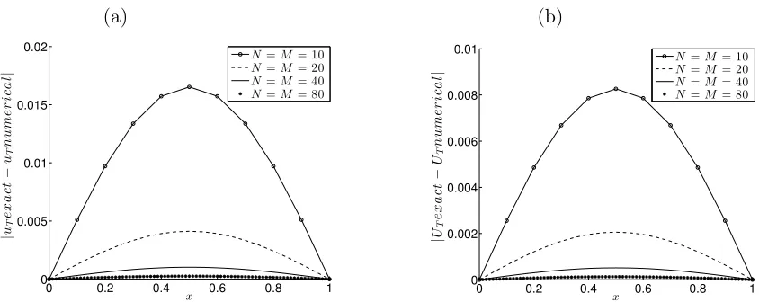
Figure 1: The absolute errors between exact and numerical solutions for (a) uT(x) and (b) UT(x), for N =M _{∈ {}10,20,40,80_} for the direct problem of Example 1.

7.1.1 Inverse problem

Since from (82) we have g _≡1, and also since T /L= 1_∈Q we do not have the uniqueness of solution of the inverse problem (79)-(81) when measuring the final displacement (85). Therefore, for Example 1 we only consider the inverse problem (79)-(81) with the time-average displacement measurement (86) which, according to the discussion in subsection 4, has a unique solution given by equations (83) and (84).

The objective function (60) given by

˜

J(fk) = 1 2||ξk||

2 ₌ 1 2

M−1 X

i=1

ξ_k2(xi), (92)

whereξk is given by (72), is plotted in Figure 2(a), as a function of the number of iterations k. From this figure it can be seen that convergence ofJ˜is achieved after about 300 iterations. Figure 2(b) shows the error between the exact solution f and numerical solution fk defined by

E(fk) =_||fexact₋fk_||= v u u t

M−1 X

i=1

(f(xi)₋fk(xi))2_{, (93)}

(a)

0 100 200 300 400 500

0 5 10 15 20

k

˜J( fk

)

(b)

0 100 200 300 400 500

0 10 20 30 40 50 60

k

E

(

fk

)

Figure 2: (a) The objective function J˜(fk) and (b) the accuracy error E(fk), versus the number of iterations k = 1,500, no noise for the inverse problem of Example 1.

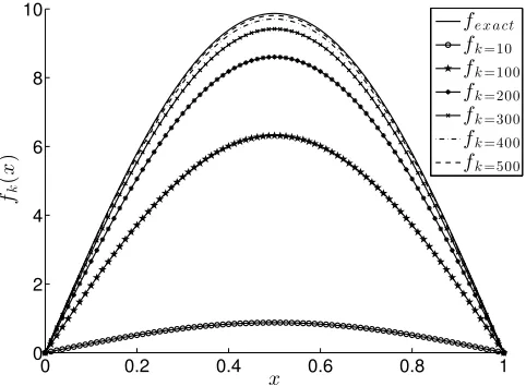
Figure 3 shows the numerical solutionfkat various iteration numbersk. From this figure a monotonic increasing convergence of the numerical solution fk towards the exact solution (83) can be clearly observed.

0 0.2 0.4 0.6 0.8 1

0 2 4 6 8 10

x fk

(

x

)

fe x a ct

fk=10

fk=100

fk=200

fk=300

fk=400

fk=500

Figure 3: The numerical solution fk at various iteration numbers k, in comparison with the exact solution (83), no noise for the inverse problem of Example 1.

In practice, the additional observation (6) comes from measurement which is inherently contaminated with errors. We therefore model this by replacing the exact data UT by the noisy data

U_Tǫ(xi) =UT(xi) +ǫi, i= 1,(M ₋1), (94)

where(ǫi)_i=1,M−1are random noisy variables generated (using the MATLAB routine ’normrd’) from a Gaussian normal distribution with mean zero and standard deviation σ = p _×

introduced in the objective functional (60) is then given by

1 2ǫ

2 ₌ 1 2

M−1 X

i=1

ǫ2_i. (95)

In order to investigate the stability of the numerical solution we include some p _∈

{10,30,50_}% noise into the input data (86), as given by equation (94). The objective functional J˜(fk) and the errors E(fk) are shown in Figure 4 for k = 1,500 iterations. In Figure 4(a) the threshold τ2ǫ2

2 (with τ = 1.15) in the stopping criterion (78) is included by

horizontal line. Intersecting the horizontal line y = τ2ǫ2

2 with the graph of the objective

functional J˜(fk) yields the stopping iteration number kdiscr given by the discrepancy prin-ciple criterion (78). On the other hand, the minimum of the curve E(fk) in Figure 4(b) yields the optimal iteration number kopt. For various percentages of noise p, the values of kdiscr and kopt together with the corresponding accuracy errors (93) are given in Table 1 for better illustrative purposes. From Figures 4(a), 4(b) and Table 1 it can be seen that there is not much difference between kopt and kdiscr for all percentages of noise p considered and this adds to the robustness of the numerical iterative method employed.

(a)

0 100 200 300 400 500

0 5 10 15 20 25 30 35 40

k

˜J( fk

)

(b)

0 100 200 300 400 500

0 10 20 30 40 50 60

k

E

(

fk

)

Table 1: The stopping iteration number kdiscr chosen according to the discrepancy principle criterion (78) (withτ = 1.15), as illustrated in Figure 4(a), and the optimal iteration number kopt chosen according to the minimum of the accuracy error function (93) in Figure 4(b) for various percentages of noise p _{∈ {}10,30,50_}% for Example 1. The corresponding accuracy errors E(fkdiscr) and E(fkopt) are also included.

p 10% 30% 50%

kopt 373 276 232

E(fkopt) 1.8471 4.2181 6.0124

kdiscr 300 245 205

E(fkdiscr) 2.5213 4.5269 6.4347

Figures 5(a) and 5(b) show the regularized numerical solution for f(x) obtained with various values of the iteration numbers listed in Table 1, namely, kopt _{∈ {}373,276,232_} and kdiscr ∈ {240,225,220}, respectively, for p∈ {10,30,50}% noisy data. From these figures it can be seen that there is not much difference obtained between the corresponding curves in Figures 5(a) and 5(b), except perhaps slightly forp= 10%. Moreover, the numerical results illustrated in Figure 5(b) reveal that stable numerical solutions are obtained if one stops the iteration process according to the discrepancy principle (78). Stability is further maintained even for large percentages of noise such as p = 50%. Furthermore, as expected, numerical results in Figure 5(b) become more accurate as the percentage of noise p decreases.

(a)

0 0.2 0.4 0.6 0.8 1

0 2 4 6 8 10

x

fk

(

x

)

fexact

fk=373, p=10% fk=276, p=30% fk=232, p=50%

(b)

0 0.2 0.4 0.6 0.8 1

0 2 4 6 8 10

x

fk

(

x

)

fexact

fk=300, p=10% fk=245, p=30% fk=205, p=50%

Figure 5: The exact solution f in comparison with the numerical solution fk for (a) kopt _∈

{373,276,232_} and (b) kdiscr _{∈ {}300,245,205_}, for p _{∈ {}10,30,50_}% noise, for the inverse problem of Example 1.

7.2

Example 2

Consider the inverse problem given by the wave equation (79) with the input data (81),

u(x,0) =ϕ(x) = sin(πx), ut(x,0) =ψ(x) = sin(πx), x_∈[0,1], (96)

and the diplacement measurement at the final time t=T = 1

u(x, t) = u(x,1) =uT(x) = sin(πx)e, x_∈[0,1], (98)

or, and the time-average displacement

Z T 0

u(x, t)dt= Z 1

0

u(x, t)dt=UT(x) = sin(πx)(e−1), x∈[0,1]. (99)

One can easily observe that the function (97) satisfies g(x, t)_≥ 0, gt(x, t)> 0,_∀(x, t)_∈ Q_T and hence, according to Theorems 1 and 2, both the inverse problems (79), (81), (96), (98), and (79), (81), (96), (99) have unique solutions. In fact, it can readily be checked by direct substitution that the analytical solution of both problems is given by

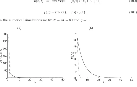
u(x, t) = sin(πx)et, (x, t)_∈[0,1]_×[0,1], (100)

f(x) = sin(πx), x_∈(0,1). (101)

In the numerical simulations we fix N =M = 80 and γ = 1.

(a)

0 10 20 30 40 50

0 50 100 150 200 250 300

k

J

(

fk

)

,

˜_J(f

k

)

(b)

0 10 20 30 40 50

0 1 2 3 4 5 6 7

k

E

(

fk

)

Figure 6: (a) The objective functions J(fk), J˜(fk) and (b) the accuracy error E(fk), versus the number of iterations k = 1,50, no noise for the inverse problem of Example 2 with the displacement measurement (98) (- - -) and with the time-average displacement measurement (99) (—).

(a)

0 0.2 0.4 0.6 0.8 1 0

0.2 0.4 0.6 0.8 1

x fk

(

x

)

fexac t

fk= 1

fk= 5

fk= 10

(b)

0 0.2 0.4 0.6 0.8 1 0

0.2 0.4 0.6 0.8 1

x fk

(

x

)

fexac t

fk= 5

fk= 10

fk= 50

Figure 7: The numerical solution fk at various iteration numbers k, in comparison with the exact solution (101), no noise for the inverse problem of Example 2 with (a) the displacement measurement (98), and (b) the time-average displacement measurement (99).

In order to investigate the stability of the numerical solutions we include some p _∈

{1,3,5_}% noise into the input data (98) (or (99)), as given by a similar expression to (94). For this noisy data, Figures 8, 9 and Table 2 are analogous to Figures 4, 5 and Table 1 of Example 1 and similar conclusions can be drawn. Stability is achieved if the iterations are stopped at the index kdiscr which is much closer to kopt for Example 2 than for Example 1 because the amount of noise is much smaller (10 times) in the former case. For the same reason, the agreement between the numerical and analytical solution is much better in Figure 9 than in Figure 5. The constant τ > 1 giving the threshold τ2_ǫ2_{/2 seems also important}

(a)

0 10 20 30 40 50

10−2 10−1 100 101 102 103

k

J

(

fk

)

(b)

0 10 20 30 40 50

10−2 10−1 100 101

k

E

(

fk

)

(c)

0 10 20 30 40 50

10−2 10−1 100 101 102

k

˜_J(f

k

)

(d)

0 10 20 30 40 50

10−2 10−1 100 101

k

E

(

fk

)

Figure 8: (a) The objective function J(fk) and (b) the corresponding accuracy error E(fk)

for the inverse problem of Example 2 with the displacement measurement (98), and (c) the objective function J˜(fk) and (d) the corresponding accuracy error E(fk) for the inverse problem of Example 2 with the time-average displace measurement (99). All curves are as functions of the number of iterations k = 1,50, for p= 1% (—), p= 3% (- - -) and p= 5%

(_{· · ·}) noise. The horizontal lines in (a) and (c) represent the threshold τ2_ǫ2_{/2 with τ = 1.15}

Table 2: The stopping iteration number kdiscr chosen according to the discrepancy principle criterion (78), as illustrated in Figures 8(a) and 8(c), and the optimal iteration number kopt chosen according to the minimum of the accuracy error function (93) in Figures 8(b) and 8(d), for various percentages of noise p _{∈ {}1,3,5_}% for Example 2 with the displacement measurement (98) andτ = 1.15(upper part of the table) and with the time-average displace-ment measuredisplace-ment (99) and τ = 1.25(lower part of the table). The corresponding accuracy errors E(fkdiscr) and E(fkopt) are also included.

p 1% 3% 5%

kopt 7 6 6

E(fkopt) 0.0102 0.0286 0.0464

kdiscr 6 5 4

E(fkdiscr) 0.0107 0.0313 0.0632

kopt 36 30 27

E(fkopt) 0.0286 0.0725 0.1102

kdiscr 33 27 24

E(fkdiscr) 0.0310 0.0778 0.1200

(a)

0 0.2 0.4 0.6 0.8 1

0 0.2 0.4 0.6 0.8 1

x

fk

(

x

)

fexact

fk=7, p=1%

fk=6, p=3%

fk=6, p=5%

(b)

0 0.2 0.4 0.6 0.8 1

0 0.2 0.4 0.6 0.8 1

x

fk

(

x

)

fexact

fk=6, p=1%

fk=5, p=3%

fk=4, p=5%

(c)

0 0.2 0.4 0.6 0.8 1

0 0.2 0.4 0.6 0.8 1

x

fk

(

x

)

fexact

fk=36, p=1% fk=30, p=3% fk=27, p=5%

(d)

0 0.2 0.4 0.6 0.8 1

0 0.2 0.4 0.6 0.8 1

x

fk

(

x

)

fexact

fk=33, p=1%

fk=27, p=3%

fk=24, p=5%

Figure 9: The numerical solution fk at various iteration numbers k, in comparison with the exact solution (101), for p _{∈ {}1,3,5_}% noise for the inverse problem of Example 2 with the displacement measurement (98) for (a) kopt _{∈ {}7,6,6_}, (b) kdiscr _{∈ {}6,5,4_}, and with the time-average displacement measurement (99) for (c) kopt _{∈ {}36,30,27_}, (d) kdiscr _∈

{33,27,24_}.

7.3

Example 3

Consider first the direct problem given by the wave equation (79) with the input data (81),

u(x,0) = ϕ(x) = sin(πx), ut(x,0) =ψ(x) = 0, x_∈[0,1], (102)

g(x, t) = 1 +t, t _∈[0,1], (103)

f(x) = 1 ˜

σ√2π exp

−(x−µ)

2 2˜σ2

where σ˜ = 0.1 and µ = 0.5. Remark that for this example, the force (104) is a Gaussian normal function with meanµand standard deviation σ. As˜ σ˜ _→0, expression (104) mimics the Dirac delta distributionδ(x₋µ).

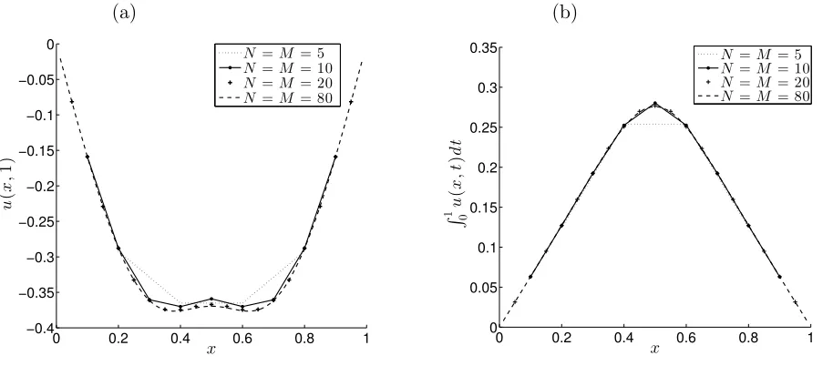
Unlike in the previous two examples, for the above direct problem an explicit analytical solution for the displacementu(x, t)is not readily available and therefore, the values (5) and (6) ofu(x,1)and R1

0 u(x, t)dt, illustrated in Figures 10(a) and 10(b), respectively, have been

obtained numerically using the FDM, at described in subsection 7.1. From these figures, a rapid convergence of the numerical results can be observed.

We next solve the inverse problems using the numerically simulated data with N =

M = 80 from Figure 10. In the numerical solutions of the direct and adjoint problems of the iterative procedure described in Section 6 we also take N = M = 80 and γ = 1. We deliberately use the same mesh discretisation N = M = 80 in order to check for exact data the numerical convergence of the Landweber method proposed in the absence of any numerical discretisation error, the only noise present being the O(10−16_{) double precision}

computer round-off errors. Note that we do not commit an inverse crime since the initial guess is arbitrary, we also add random noise to the input data and the inverse iterative procedure is totally different than the direct problem solver.

(a)

0 0.2 0.4 0.6 0.8 1

−0.4 −0.35 −0.3 −0.25 −0.2 −0.15 −0.1 −0.05 0

x

u

(

x

,

1

)

N=M = 5

N=M = 10

N=M = 20

N=M = 80

(b)

0 0.2 0.4 0.6 0.8 1

0 0.05 0.1 0.15 0.2 0.25 0.3 0.35

x

R1 0

u

(

x

,

t

)

d

t

N=M = 5

N=M = 10

N=M = 20

N=M = 80

Figure 10: Numerical solution for (a) u(x,1) and (b) R1

0 u(x, t)dt, for various N = M ∈

{5,10,20,80_}, for the direct problem of Example 3.

7.3.1 Inverse problems

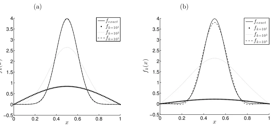
As in Example 2, the function (103) satisfiesg(x, t)_≥0, gt(x, t)>0,_∀(x, t)_∈QT and hence, according to Theorems 1 and 2, both the inverse problems (79), (81), (102) with the input (5) or (6) represented in Figure 10(a) or 10(b), respectively, have unique solutions. First consider the case without noise, i.e. p = 0. Figure 11 shows the objective functions (47) and (60), and the corresponding accuracy error (93), versus the number of iterations. Also, Figure 12 shows the convergence of the corresponding numerical solutions, as the number of iterations increases. From both figures it can be seen that the number of iterations necessary to achieve a high level of accuracy is large ofO(105_{). It is much larger than in the previous Examples 1}

therefore a sharper peak centred at the mean valueµ= 0.5than the trigonometric functions (83) and (101). By comparing the results in Figures 11 and 12 one can also observe that the convergence for the inverse problem with the displacement measurement (5) is much faster (and for some number of iteration more accurate) than that with time-average displacement measurement (29).

(a)

100 101 102 103 104 105

10−8 10−6 10−4 10−2 100 102

k

J

(

fk

)

,

˜_J(f

k

)

(b)

100 101 102 103 104 105

10−1 100 101 102

k

E

(

fk

)

Figure 11: (a) The objective functions J(fk),J˜(fk)and (b) the accuracy errorE(fk), versus the number of iterations k = 1,105_{, no noise for the inverse problem of Example 3 with the}

displacement measurement (5) (- - -) and with the time-average displacement measurement (29) (—).

(a)

0 0.2 0.4 0.6 0.8 1

−0.5 0 0.5 1 1.5 2 2.5 3 3.5 4

x fk

(

x

)

fexact fk=101

fk=103

fk=105

(b)

0 0.2 0.4 0.6 0.8 1

−0.5 0 0.5 1 1.5 2 2.5 3 3.5 4

x fk

(

x

)

fexact fk=101

fk=103

fk=105

Figure 12: The numerical solutionfkat various iteration numbers k, in comparison with the exact solution (104), no noise for the inverse problem of Example 3 with (a) the displacement measurement (5), and (b) the time-average displacement measurement (29).

similar quantitative conclusions can be drawn in terms of comparing the inverse problems with either the displacement measurement (5) numerically simulated in Figure 10(a) or with the time-average measurement (29) numerically simulated in Figure 10(b). Of course, since more iterations are required for Example 3 than for Example 2, the thresholdskdiscr andkopt are much higher (and also more different between themselves) in Table 3 than in Table 2. Furthermore, the accuracy of the numerical results in Figure 9 for Example 2 is much higher than that in Figure 14 for Example 3, as expected since the trigonometric source (101) is less complicated than the Gaussian normal bell-shaped function (104).

(a)

100 101 102 103 104 105 10−4

10−3 10−2 10−1 100 101

k

J

(

fk

)

(b)

100 101 102 103 104 105

0 5 10 15

k

E

(

fk

)

(c)

100 101 102 103 104 105 10−4

10−3 10−2 10−1 100 101

k

˜J( fk

)

(d)

100 101 102 103 104 105

0 5 10 15

k

E

(

fk

)

Figure 13: (a) The objective functionJ(fk)and (b) the corresponding accuracy error E(fk)

for the inverse problem of Example 3 with the displacement measurement from Figure 10(a) with N =M = 80, and (c) the objective function J˜(fk)and (d) the corresponding accuracy errorE(fk)for the inverse problem of Example 3 with the time-average displace measurement of Figure 10(b) with N = M = 80. All curves are functions of the number of iterations k = 1,105_{, for p= 1% (—), p= 3% (- - -) and p= 5% (· · ·) noise. The horizontal lines in}

Table 3: The stopping iteration number kdiscr chosen according to the discrepancy principle criterion (78), as illustrated in Figures 13(a), 13(c), and the optimal iteration number kopt chosen according to the minimum of the accuracy error function (93) in Figures 13(b), 13(d), for various percentages of noise p _{∈ {}1,3,5_}% for Example 3 with the displacement measurement from Figure 10(a) withN =M = 80andτ = 1.2(upper part of the table) and with the time-average displacement measurement from Figure 10(b) with N =M = 80 and τ = 1.1 (lower part of the table). The corresponding accuracy errors E(fkdiscr) and E(fkopt)

are also included.

p 1% 3% 5%

kopt 34080 20363 15577 E(fkopt) 0.5899 1.3122 1.9840

kdiscr 17712 7949 7012

E(fkdiscr) 0.9448 2.0762 2.5206

kopt 95908 49208 26760

E(fkopt) 1.1314 2.6532 3.8913

kdiscr 64996 35905 14998

(a)

0 0.2 0.4 0.6 0.8 1

−0.5 0 0.5 1 1.5 2 2.5 3 3.5 4 x fk ( x ) fexact

fk=34080, p=1%

f_{k=20363, p=3%}

f_{k=15577, p=5%}

(b)

0 0.2 0.4 0.6 0.8 1

−0.5 0 0.5 1 1.5 2 2.5 3 3.5 4 x fk ( x ) fexact

fk=17712, p=1%

fk=7949, p=3%

fk=7012, p=5%

(c)

0 0.2 0.4 0.6 0.8 1

−0.5 0 0.5 1 1.5 2 2.5 3 3.5 4 x fk ( x ) fexact

fk=95908, p=1%

fk=49208, p=3%

fk=26760, p=5%

(d)

0 0.2 0.4 0.6 0.8 1

−0.5 0 0.5 1 1.5 2 2.5 3 3.5 4 x fk ( x ) fexact

fk=64996, p=1%

fk=35905, p=3%

fk=14998, p=5%

Figure 14: The numerical solution fk at various iteration numbers k, in comparison with the exact solution (104), for p _{∈ {}1,3,5_}% noise for the inverse problem of Example 3 with the displacement measurement from Figure 10(a) with N = M = 80 for (a) kopt _∈

{34080,20363,15577_}, (b) kdiscr ∈ {17712,7949,7012}, and with the time-average displace-ment measuredisplace-ment from Figure 10(b) withN =M = 80for (c)kopt _{∈ {}95908,49208,26760_}, (d) kdiscr _{∈ {}64996,35905,14998_}.

7.4

Example 4

Consider first the direct problem given by the wave equation (79) with the input data (81),

u(x,0) =ϕ(x) = 0, ut(x,0) =ψ(x) = 0, x_∈[0,1], (105)

g(x, t) = 1 +t, t _∈[0,1], (106)

f(x) = (

x if 0_≤x_≤ 1₂,

Remark that for this example, the force (107) has a triangular shape, being continuous but non-differentiable at the peak x = 1/2. This example also does not possess an explicit analytical solution for the displacement u(x, t) being readily available.

0 0.2 0.4 0.6 0.8 1 0

0.02 0.04 0.06 0.08 0.1 0.12 0.14

x

u

(

x

,

1

)

N =M = 5

N =M = 10

N =M = 20

N =M = 80

Figure 15: Numerical solution foru(x,1), for variousN =M _{∈ {}5,10,20,80_}, for the direct problem of Example 4.

Figure 15 shows the rapid convergence of the FDM numerical solution u(x,1) of the direct problem (79), (81) and (105), as N =M increases. The numerically simulated u(x,1)

with N =M = 80 is used as input data (5) in the inverse problem (79), (81), (105) whose existence and uniqueness of solution is guaranteed from Theorem 1 since g(x, t) given by (106) satisfiesg(x, t)_≥0, gt(x, t)>0,_∀(x, t)_∈QT. We fix N =M = 80 and γ = 1.

It was observed in Example 3 and else where that the convergence of the Landweber iterative method described in Section 6 can become prohibitely show. One way to increase the rate of convergence is to increase the value of the relaxation parameter γ in (74) and we shall investigate this effect for the next Example 5. Alternatively, one can speed up the convergence of the minimization of the least-squares functional (47) or (60) by employing the convergent and regularizing conjugate gradient method (CGM) for the stable reconstruction of the displacement u and force f. In addition, the CGM does not require any choice of a relaxation parameter γ, as the Landweber method does in order to iterate in formula (74). Similarly, as described in [8, 12] for the heat equation, this algorithm runs as follows:

Let steps (i) and (ii) be the same as in the algorithm of Section 6. The next steps are as follows:

(iii) Calculate

dk(x) = ₋zk(x) +βk₋1dk−1(x), (108)

with the convention that β₋1 = 0 and

βk₋1 =

||zk||2L2_(Ω)

||zk₋1||2_L2

(Ω)

(iv) Solve the direct problem (1)-(4) with ϕ = ψ = 0 and f = dk to determine A0dk or

˜

A0dk, where the operatorsA0 and A˜0 have been defined in Section 3. Set the direction

search

αk= ||zk|| 2

L2_(Ω)

||A0dk||2_L2

(Ω)

, or αk = ||zk|| 2

L2_(Ω)

||A˜0dk||2_L2

(Ω)

, k _≥0, (110)

and pass to the new iteration by letting

fk+1(x) = fk(x) +αkdk(x). (111)

(v) Let uk+1 solve the direct problem (1)-(4) with f = fk+1 and go back (repeat) steps

(ii)-(iv) until the discrepancy principle stopping criterion (78) is satisfied.

Note that for Ω = (0, L) the L2_{(0, L) integrals in (109) and (110) are calculated using the}

trapezoidal rule which, for the homogeneous Dirichlet boundary data (81), is given by

||zk_||2_L2_(0,L)= (∆x) M−1

X

i=1

z_k2(xi), (112)

and a similar expression exists for _||A0dk||2_L2_(0,L).

(a)

100 101 102 103 104 105

10−10

10−8

10−6

10−4

10−2

100

k

J

(

fk

)

(b)

100 101 102 103 104 105 10−2

10−1 100 101

k

E

(

fk

)

Figure 16: (a) The objective function J(fk) and (b) the accuracy error E(fk), versus the number of iterations k = 1,105_{, obtained using the Landweber method (—) and the CGM}

(a)

0 0.2 0.4 0.6 0.8 1

0 0.1 0.2 0.3 0.4 0.5

x fk

(

x

)

fexact f_k=101

fk=103

f_k=105

(b)

0 0.2 0.4 0.6 0.8 1

0 0.1 0.2 0.3 0.4 0.5

x fk

(

x

)

fexact fk=101

f_k=103

f_k=105

Figure 17: Numerical solution fk for various iteration numbers k _{∈ {}101_,103_,105_{}, in}

com-parison with the exact solution (107), obtained using (a) the Landweber method and (b) the CGM, no noise for the inverse problem of Example 4.

The objective function (47), the accuracy error (93) and the numerical solution for the force at various iteration numbers obtained using the Landweber method and the CGM are plotted in Figures 16(a), 16(b) and 17, respectively. From these figures it can be seen that it takes a large number of iterations of O(105_{) to converge with a good accuracy to}

the exact solution (107), similarly to what happened for Example 3, when the Lanweber method is employed. In comparison to the previous Examples 1 and 2 this is to be expected because the force function (107) to be retrieved is non-smooth possessing a sharp corner at the peakx= 1/2. Moreover, the behaviour of the convergence is similar to that of Example 3 for which the Gaussian normal force function (104) to be retrieved, although smooth, it possesses also a sharp peak at x= 1/2.

(a)

100 101 102 103 104 105 10−5

10−4 10−3 10−2 10−1 100

k

J

(

fk

)

(b)

100 101 102 103 104 105

0 0.5 1 1.5 2 2.5

k

E

(

fk

)

(c)

100 101 102 103 104 105

10−5

10−4

10−3

10−2

10−1

100

k

J

(

fk

)

(d)

100 101 102 103

0 0.5 1 1.5 2 2.5

k

E

(

fk

)

Figure 18: (a) and (c) The objective function J(fk), and (b) and (d) the accuracy error E(fk), versus the number of iterations k= 1,105_{, obtained using the Landweber and CGM}

methods, respectively, for p= 1%(—), p= 3%(- - -) and p= 5% (_{· · ·}) noise for the inverse problem of Example 4. The horizontal lines represents the threshold τ2ǫ2

2 with τ = 1.15.

Table 4: The stopping iteration numberskdiscr chosen according to the discrepancy principle criterion (78) (with τ = 1.15), as illustrated in Figures 18(a) and 18(c), and the optimal iteration numberskopt chosen according to the minimum of the accuracy error function (93) in Figures 18(b) and 18(d), for various percentages of noise p _{∈ {}1,3,5_}% for Example 4. The corresponding accuracy errors E(fkdiscr) and E(fkopt) are also included. The CGM

results are included in brackets

p 1% 3% 5%

kopt 10171 3429 68

(2908) (295) (12)

E(fkopt) 0.1202 0.3009 0.3198

(0.1090) (0.2943) (0.3167)

kdiscr 2995 95 70

(130) (21) (11)

E(fkdiscr) 0.1507 0.3105 0.3199

(a)

0 0.2 0.4 0.6 0.8 1

0 0.1 0.2 0.3 0.4 0.5

x

fk

(

x

)

fexact

fk=10171, p=1%

fk=3429, p=3%

fk=68, p=5%

(b)

0 0.2 0.4 0.6 0.8 1

0 0.1 0.2 0.3 0.4 0.5

x

fk

(

x

)

fexact

fk=2995, p=1% fk=95, p=3% fk=70, p=5%

(c)

0 0.2 0.4 0.6 0.8 1

0 0.1 0.2 0.3 0.4 0.5

x

fk

(

x

)

fexact

fk=2908, p=1%

fk=295, p=3% fk=12, p=5%

(d)

0 0.2 0.4 0.6 0.8 1

0 0.1 0.2 0.3 0.4 0.5

x

fk

(

x

)

fexact

fk=130, p=1% fk=21, p=3% fk=11, p=5%

Figure 19: The exact solution f in comparison with numerical solution fk for (a) and (c) kopt _{∈ {}10171,3429,68_} and kopt _{∈ {}2908,295,12_}, and (b) and (d) kdiscr _{∈ {}2995,95,70_}

and kdiscr _{∈ {}130,21,11_}, obtained using the Landweber and CGM methods, respectively, for p_{∈ {}1,3,5_}%noise for the inverse problem of Example 4.

We finally note that similar results have been obtained for the inverse problem given by equations (79), (81), (105) with the integral measurement (29) and therefore, they are not presented.

7.5

Example 5

The previous example investigated a severe test given by the non-smooth triangular shape force function (107). In this subsection, we consider an even more severe test example given by the discontinuous force

f(x) =     

0 if 0_≤x < 1₃,

1 if 1_{3 ≤}x_≤ 2₃,

0 if 2₃ < x_≤1.

We take the same input data (105) and (106), as in Example 4. Then, on solving the direct problem given by equations (79), (81), (105) with the forcing term given by the product of the functions in (106) and (113), we obtain the numerical results for the time-average displacement R1

0 u(x, t)dt illustrated in Figure 20. From this figure it can be seen that a

convergent FDM numerical solution is achieved.

For brevity, in what follows we only illustrate the numerical results obtained for the inverse problem (1)-(4), (29), noting that similar results have been obtained for the inverse problem (1)-(5).

0 0.2 0.4 0.6 0.8 1

0 0.01 0.02 0.03 0.04 0.05 0.06 0.07 0.08

x

R1 u0

(

x

,

t

)

d

t

N =M = 5

N =M = 10

N =M = 20

N =M = 80

Figure 20: Numerical solution for R1

0 u(x, t)dt, for various N = M ∈ {5,10,20,80}, for the

direct problem of Example 5.

The numerically simulated data forR1

0 u(x, t)dt obtained withN =M = 80is used as

in-put (6) in the inverse problem given by equations (79), (81) and (105). Again, as in Examples 2 and 3 the functionggiven by equation (103) (or (106)) satisfies0_6≡g(x, t)_≥0,_∀(x, t)_∈QT and hence, according to Theorem 2, the inverse problem has a unique solution. As expected, for exact data a very slow convergence of the objective function (60) is encountered by the Landweber iteration method because the force function (113) to be retrieved is discontinuous at the points x_{∈ {}1/3,2/3_}. In fact, we had to increase the value of the relaxation factor γ in order to achieve convergence in a reasonable number of iterations.

Figure 21 shows the objective function (60) and the accuracy error (93), versus the number of iterationsk = 1,105_{, for various values of the relaxation parameterγ ∈ {1,5,15}.}

From this figure it can be seen that the rate of convergence increases as we increase γ from 1 to 5 and then to 15. The corresponding numerical solutions for the force fk(x)are shown in Figure 22 for various numbers of iterations k _{∈ {}101_,103_,105_{}, and again more accurate}

(a)

100 101 102 103 104 105

10−8

10−6

10−4

10−2

100

k

˜J( fk

)

(b)

100 101 102 103 104 105

1 2 3 4 5 6

k

E

(

fk

)

Figure 21: (a) The objective function J˜(fk) and (b) the accuracy error E(fk), versus the number of iterations k = 1,105_{, for various γ = 1 (—), γ = 5 (- - -) and γ = 15 (− • −), no}

(a)

0 0.2 0.4 0.6 0.8 1

−0.2 0 0.2 0.4 0.6 0.8 1 1.2

x fk

fexac t

fk= 1 01

f_k= 1 03

f_k= 1 05

(b)

0 0.2 0.4 0.6 0.8 1

−0.2 0 0.2 0.4 0.6 0.8 1 1.2

x fk

fexac t

fk= 1 01

f_k= 1 03

f_k= 1 05

(c)

0 0.2 0.4 0.6 0.8 1

−0.2 0 0.2 0.4 0.6 0.8 1 1.2

x fk

fexac t

fk= 1 01

fk= 1 03

fk= 1 05

Figure 22: Numerical solution fk for various iteration numbers k ∈ {101,103,105}, in com-parison with the exact solution (113), for (a) γ = 1, (b) γ = 5 and (c) γ = 15, no noise for the inverse problem of Example 5.

In order to investigate the stability of the numerical solution we include some p _∈