Congestion analysis for low power and lossy networks

(1)

This is a repository copy of

Congestion analysis for low power and lossy networks

.

White Rose Research Online URL for this paper:

http://eprints.whiterose.ac.uk/103651/

Version: Accepted Version

Proceedings Paper:

Al-Kashoash, HAA orcid.org/0000-0001-9681-8285, Al-Nidawi, Y and Kemp, AH (2016)

Congestion analysis for low power and lossy networks. In: 2016 Wireless

Telecommunications Symposium (WTS). 2016 Wireless Telecommunications Symposium

(WTS), 18-20 Apr 2016, London, UK. IEEE . ISBN 9781509003143

https://doi.org/10.1109/WTS.2016.7482027

eprints@whiterose.ac.uk https://eprints.whiterose.ac.uk/

Reuse

Unless indicated otherwise, fulltext items are protected by copyright with all rights reserved. The copyright exception in section 29 of the Copyright, Designs and Patents Act 1988 allows the making of a single copy solely for the purpose of non-commercial research or private study within the limits of fair dealing. The publisher or other rights-holder may allow further reproduction and re-use of this version - refer to the White Rose Research Online record for this item. Where records identify the publisher as the copyright holder, users can verify any specific terms of use on the publisher’s website.

Takedown

If you consider content in White Rose Research Online to be in breach of UK law, please notify us by

(2)

Congestion Analysis for Low Power and Lossy

Networks

Hayder A. A. Al-Kashoash

a,b

_{Yaarob Al-Nidawi}

a

_{and Andrew H. Kemp}

a

a _{School of Electronic and Electrical Engineering}

University of Leeds, Leeds, UK

Email:{ml14haak, elymna, a.h.kemp}@leeds.ac.uk

b

Southern Technical University, Basra, Iraq

Abstract—Low Power and Lossy Networks (LLNs) represent

one of the interesting research areas in recent years. The IETF ROLL and 6LoWPAN working groups have developed new IP based protocols for LLNs such as the RPL routing protocol. In LLNs e.g. 6LoWPANs, heavy data traffic causes congestion which significantly degrades network performance. In this paper, we explore the impact of congestion on 6LoWPAN networks where an extensive analysis is carried out with different scenarios and parameters. Analysis results show that when congestion occurs, the majority of packets are lost due to buffer overflow as compared to channel loss. Also, we found that when the application payload length is increased since IPv6 packets are fragmented, the reassembly timeout parameter value has a significant effect on network performance. Thus, it is important to consider buffer occupancy and the reassembly timeout parameter in protocol design, e.g. RPL, to improve network performance when congestion does occur.

I. INTRODUCTION

Recently, LLNs such as IPv6 over low power wireless personal area networks (6LoWPANs) have been recognized as an important and challenging research area. LLNs are used in different applications, ranging from wireless healthcare to energy metering on the smart grid [1]. 6LoWPAN supports the use of the TCP/IP architecture for wireless sensor nodes and therefore it can participate in the Internet of Things (IoT) [2]. However, when 6LoWPAN works with the TCP/IP model, sensor nodes face many issues and problems due to energy and buffer resources limitation. The Internet uses TCP (trans-mission control protocol) and UDP (user datagram protocol) as transport protocols where TCP has a congestion control mechanism and UDP does not provide any congestion control scheme. However, as TCP requires connection setup and termi-nation before and after the data transmission, it is considered inefficient for 6LoWPAN networks [3]. Therefore, one of the main issues in 6LoWPAN is congestion which causes packet loss, energy consumption and decreased throughput.

In this paper, we are addressing the problem of congestion in 6LoWPAN networks. The impact of congestion on 6LoWPAN has been evaluated with regards to different sized networks and various parameters and scenarios. Results show that with high network traffic, the majority of packets are lost at node buffers due to buffer overflow. Therefore, it is important to take buffer

occupancy into account in protocol design (e.g. IPv6 Routing Protocol for LLNs (RPL)) to reduce the number of dropped packets at the buffer. Also, simulation results show that the value of the reassembly timeout parameter has significant impact on network performance when congestion occurs as an IPv6 packet is fragmented by SICSlowpan adaptation layer. In [4], Teo et al. propose a new reassembly mechanism called Multi-Reassemblies Buffer Management System (MR-BMS) for 6LoWPAN networks. MR-BMS consists of three components: buffer manager, list of reassembly buffer and IP packet buffer. When a new fragment arrives at a node, the buffer manager creates a new reassembly buffer to store the incoming fragment and starts a reassembly timer. After that, if the next incoming fragment belongs to the packet of the first fragment, it is stored in the same buffer. Otherwise, a new reassembly buffer is created to store the incoming fragment. However, the authors do not show the importance of the reassembly timeout parameter value in heavy data traffic conditions.

The remainder of the paper is organized as follows: in section 2, we present the results of congestion analysis in 6LoWPAN with and without fragmentation. Then, section 3 discusses simulation results and finally, section 4 concludes this paper and indicates future work.

II. CONGESTIONANALYSIS IN6LOWPAN NETWORKS

Congestion occurs when multiple sensor nodes start to send packets concurrently at high data rate or when a node relays many flows across the network. Thus, link collision on the wireless channel and packet overflow at buffer nodes occur in the network [5]. Recently, few papers have been presented to investigate and address congestion in 6LoWPAN networks [6], [7], [8], [9], but none considered congestion assessment and analysis. In [10], Hull et al. did a testbed experiment in a traditional wireless sensor network protocol stack with TinyOS where B-MAC and single destination DSDV (Destination Sequenced Distance Vector) routing protocol are used. In this paper, experiments in 6LoWPAN wireless sensor network using a protocol stack as shown in table I and the Contiki OS [11] are considered.

(3)

[image:3.612.327.559.50.169.2]

TABLE I: Protocol stack

Layer Protocol Parameter value

Application Every node periodically send packet to sink node

Transport UDP

Network uIPv6 + RPL objective function = MHROF

Adaptation SICSlowpan layer compression method = HC06

Data Link CSMA ( MAC layer)

Contikimac (RDC layer) 802.15.4 (framer)

buffer size = 8 packets CCA count = 2 MAC retransmission = 3 channel check rate = 8 Hz

[image:3.612.47.301.67.232.2]

Physical CC2420 RF transceiver Max. packet length = 127 byte

TABLE II: Simulation parameters

Parameter Value

Simulation time 30 minutes for each simulation

Ratio model UDGM - Distance Loss

Node type Tmote Sky

Transmission range 50 m

Interference range 100 m

simulator [12] with different network sizes and various offered loads were performed. In the networks, an average number

of nodes per personal operating space (POS)1 is 4. These

experiments have been executed with and without fragmen-tation which is implemented at the SICSlowpan (adapfragmen-tation) layer. The SICSlowpan layer performs two main functions: IPv6 header compression [14] and IPv6 fragmentation and reassembly [15]. Before an IPv6 packet is transmitted over an 802.15.4 link, the IPv6 header must be compressed by using a compression header mechanism. After compression, if the IPv6 packet size does not fit into a single 802.15.4 frame size, it must be fragmented. In each network, every node sends packets periodically to a single sink node. The protocol stack and simulation parameters which have been used in the

experiments are shown in tables I and II. Cooja simulator

implements a number of wireless channel models such as Unit Disk Graph Medium (UDGM) - Distance Loss which is used in the simulation since interference is considered [16]. In UDGM - Distance Loss, the transmission range is modelled as a disk where all nodes inside the disk can transmit and receive packets with probability of SUCCESS RATIO TX and SUCCESS RATIO RX respectively. In the Contiki OS, all sending and receiving packets are stored in a common buffer called the Rime buffer which contains the application data and packet attributes such as RSSI value [17]. Some protocols, which need to queue packets, can allocate a queue buffer to store waiting packets such as the MAC protocol that cannot send packets until the wireless channel becomes free.

A. Without Fragmentation

In this subsection, we present the congestion analysis results without fragmentation where each single IPv6 packet sends

1_{The POS is defined as a physical space (coverage area) of a node since} other nodes inside this area can communicate with the node [13]

0 10 20 30 40 50 60 70 80 90 100 1 5 -n o d e s 2 5 -n o d e s 5 0 -n o d e s 1 5 -n o d e s 2 5 -n o d e s 5 0 -n o d e s 1 5 -n o d e s 2 5 -n o d e s 5 0 -n o d e s 1 5 -n o d e s 2 5 -n o d e s 5 0 -n o d e s 1 5 -n o d e s 2 5 -n o d e s 5 0 -n o d e s 1 5 -n o d e s 2 5 -n o d e s 5 0 -n o d e s 1 5 -n o d e s 2 5 -n o d e s 5 0 -n o d e s 1 5 -n o d e s 2 5 -n o d e s 5 0 -n o d e s 1 5 -n o d e s 2 5 -n o d e s 5 0 -n o d e s 1 5 -n o d e s 2 5 -n o d e s 5 0 -n o d e s

1/64 1/32 1/16 1/8 1/4 1/2 1/1 2/1 4/1 8/1

P a ck e t Lo st (% )

Offered load per node (packet/second)

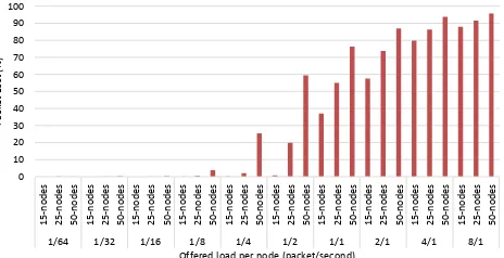
Fig. 1: Packet loss [buffer size = 8 packets]

1 10 100 1000 10000 100000 1000000 1 5 -n o d e s 2 5 -n o d e s 5 0 -n o d e s 1 5 -n o d e s 2 5 -n o d e s 5 0 -n o d e s 1 5 -n o d e s 2 5 -n o d e s 5 0 -n o d e s 1 5 -n o d e s 2 5 -n o d e s 5 0 -n o d e s 1 5 -n o d e s 2 5 -n o d e s 5 0 -n o d e s 1 5 -n o d e s 2 5 -n o d e s 5 0 -n o d e s 1 5 -n o d e s 2 5 -n o d e s 5 0 -n o d e s 1 5 -n o d e s 2 5 -n o d e s 5 0 -n o d e s 1 5 -n o d e s 2 5 -n o d e s 5 0 -n o d e s 1 5 -n o d e s 2 5 -n o d e s 5 0 -n o d e s

1/64 1/32 1/16 1/8 1/4 1/2 1/1 2/1 4/1 8/1

N u m b e r o f lo st p a ck e ts

Offered load per node (packet/second) Buffer overflow Channel loss

Fig. 2: Number of lost packets in buffer and wireless channel [buffer size = 8 packets]

over a one 802.15.4 frame without fragmentation. The network sizes are set to be 15, 25 and 50 nodes and the offered loads (packet/second) are 8/1, 4/1, 2/1, 1/1, 1/2, 1/4, 1/8, 1/16, 1/32, and 1/64.

Firstly, we set the MAC buffer size to 8 packets (8 * 127 bytes) which is the default setting of the Contiki OS. Fig. 1 shows the packet loss in 15-node, 25-node and 50-node networks respectively. Clearly, as offered load and number of nodes increase, the packet loss rises in the network. For example, with an offered load of one packet every second, the packet loss increases from 37% to 76% as the number of nodes in the network increases from 15 to 50. Fig. 2 shows the number of lost packets, which are measured at the MAC layer, due to buffer drops and channel loss. In this figure, a logarithmic scale is used due to the big difference between packet buffer drops and packet channel loss. It is clear that with high offered load, the number of packets which are lost at sensor nodes (due to buffer overflow) is much higher than the lost packets in the wireless channel. For instance, when the offered load is 8 packets per second and network size of 50 nodes, the total number of lost packets are up to 600,000 due to buffer overflow compared with only 2,000 due to channel loss. However, with low offered load, the number of lost packets in the wireless channel is slightly higher than due to buffer drops e.g. with network traffic of 1 packet per 16 seconds and 50-node network, the lost packets due to buffer overflow

and channel loss are 3 and 18 respectively. From Fig. 2,

[image:3.612.323.557.201.322.2]

(4)

0 10 20 30 40 50 60 70 80 90 100 1 5 -n o d e s 2 5 -n o d e s 5 0 -n o d e s 1 5 -n o d e s 2 5 -n o d e s 5 0 -n o d e s 1 5 -n o d e s 2 5 -n o d e s 5 0 -n o d e s 1 5 -n o d e s 2 5 -n o d e s 5 0 -n o d e s 1 5 -n o d e s 2 5 -n o d e s 5 0 -n o d e s 1 5 -n o d e s 2 5 -n o d e s 5 0 -n o d e s 1 5 -n o d e s 2 5 -n o d e s 5 0 -n o d e s 1 5 -n o d e s 2 5 -n o d e s 5 0 -n o d e s 1 5 -n o d e s 2 5 -n o d e s 5 0 -n o d e s 1 5 -n o d e s 2 5 -n o d e s 5 0 -n o d e s

1/64 1/32 1/16 1/8 1/4 1/2 1/1 2/1 4/1 8/1

P a ck e t Lo st (% )

[image:4.612.65.293.48.168.2]

Offered load per node (packet/second)

Fig. 3: Packet loss [buffer size = 16 packets]

1 10 100 1000 10000 100000 1000000 1 5 -n o d e s 2 5 -n o d e s 5 0 -n o d e s 1 5 -n o d e s 2 5 -n o d e s 5 0 -n o d e s 1 5 -n o d e s 2 5 -n o d e s 5 0 -n o d e s 1 5 -n o d e s 2 5 -n o d e s 5 0 -n o d e s 1 5 -n o d e s 2 5 -n o d e s 5 0 -n o d e s 1 5 -n o d e s 2 5 -n o d e s 5 0 -n o d e s 1 5 -n o d e s 2 5 -n o d e s 5 0 -n o d e s 1 5 -n o d e s 2 5 -n o d e s 5 0 -n o d e s 1 5 -n o d e s 2 5 -n o d e s 5 0 -n o d e s 1 5 -n o d e s 2 5 -n o d e s 5 0 -n o d e s

1/64 1/32 1/16 1/8 1/4 1/2 1/1 2/1 4/1 8/1

Fig. 4: Number of lost packets in buffer and wireless channel [buffer size = 16 packets]

can see that with high traffic, the majority of packets are lost at the buffer i.e. more than 90% of the total lost packets are lost due to buffer overflow.

Secondly, we increase the buffer size to 16 packets to see the impact of buffer size on the lost packets at the buffer. Fig. 3 shows packet loss with number of different network sizes and offered loads. By comparing Fig. 1 with Fig. 3, it can be seen that by doubling the buffer size, the packet loss decreases with different offered loads. Similarly, the number of dropped packets at the buffer decreases by a small amount as can be

seen by comparing Fig. 2 and Fig. 4. With the 8-packet

buffer size scenario, more than 90% of lost packets occurs in the buffer with offered load 8/1, 4/1, 2/1 and 1/1. However, by increasing the buffer size, the number of lost packets due to buffer overflow is still dominant as compared with channel loss.

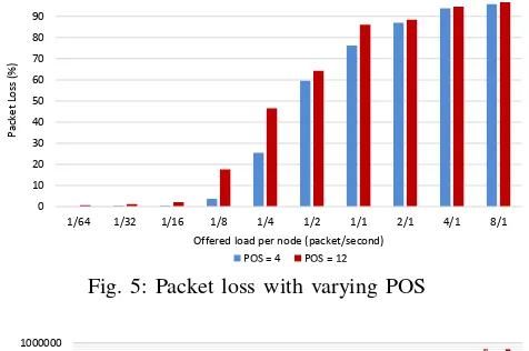
Finally, we increase the node density with an average number of nodes per POS to 12, as node density has an impact on contention among nodes to access the wireless channel. We simulate a new network with 50 nodes and POS of 12 and compare it with the 50-node network which has POS of 4. From Fig. 5, we can see that packet loss increases with high POS. Also, the number of lost packets in both the buffer and the wireless channel increases as shown in Fig. 6.

B. With Fragmentation

Next, in order to see the impact of increasing the application payload length such IPv6 packet is fragmented on network per-formance within congestion. The application payload length is

0 10 20 30 40 50 60 70 80 90 100

1/64 1/32 1/16 1/8 1/4 1/2 1/1 2/1 4/1 8/1

P a ck e t Lo ss (% )

[image:4.612.322.560.55.213.2]

Offered load per node (packet/second) POS = 4 POS = 12

Fig. 5: Packet loss with varying POS

1 10 100 1000 10000 100000 1000000 POS = 4 POS = 12 POS = 4 POS = 12 POS = 4 POS = 12 POS = 4 POS = 12 POS = 4 POS = 12 POS = 4 POS = 12 POS = 4 POS = 12 POS = 4 POS = 12 POS = 4 POS = 12 POS = 4 POS = 12

1/64 1/32 1/16 1/8 1/4 1/2 1/1 2/1 4/1 8/1

Fig. 6: Number of lost packets in buffer and wireless channel with varying POS

increased since every IPv6 packet is fragmented into two or more fragments where each fragment is sent over a single 802.15.4 frame. In these experiments, 5-node, 15-node and 25-node networks as well as 8/1, 4/1, 2/1, 1/1, 1/2, 1/4, 1/8, 1/16, 1/32, and 1/64 offered loads (packet/second) are used.

[image:4.612.61.294.201.322.2]

(5)

0 2000 4000 6000 8000 10000 12000 14000 16000 18000 20000

1/64 1/32 1/16 1/8 1/4 1/2 1/1 2/1 4/1 8/1

N

u

m

b

e

r

o

f

re

ce

iv

e

d

p

a

ck

e

ts

a

t

si

n

k

Offered load (packet/second)

0.001 0.005 0.05 0.5 1 10 30 60

[image:5.612.64.289.49.168.2]

Reassembly timeout (seconds)

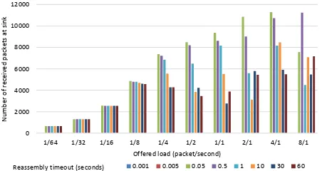
Fig. 7: Number of received packets (when broken into two fragments) at sink in 5-node network

0 2000 4000 6000 8000 10000 12000 14000

1/64 1/32 1/16 1/8 1/4 1/2 1/1 2/1 4/1 8/1

N

u

m

b

e

r

o

f

re

ce

iv

e

d

p

a

ck

e

ts

a

t

si

n

k

0.001 0.005 0.05 0.5 1 10 30 60

[image:5.612.329.552.49.168.2]

0 2000 4000 6000 8000 10000 12000

1/64 1/32 1/16 1/8 1/4 1/2 1/1 2/1 4/1 8/1

N

u

m

b

e

r

o

f

re

ce

iv

e

d

p

a

ck

e

ts

a

t

si

n

k

0.001 0.005 0.05 0.5 1 10 30 60

In 6LoWPAN, the routing schemes can be divided into two categories: ’route over’ and ’mesh under’ [18]. With route over, the routing decision is made at the routing layer and the fragmentation and reassembly process is implemented at each node through path from source to destination. In mesh under, the routing decision is taken at SICSlowpan layer (adaptation layer) as well as fragmentation and reassembly being executed at source and destination nodes only. The Contiki OS supports the ’route over’ scheme, which is used in these experiments, where RPL performs the routing decision.

Firstly, the application payload length is set to 100 bytes since every IPv6 packet is divided into two fragments. Figures

7, 8 and 9 show the number of received packet at the

sink node with different offered loads and various reassembly

0 1000 2000 3000 4000 5000 6000 7000 8000 9000

1/64 1/32 1/16 1/8 1/4 1/2 1/1 2/1 4/1 8/1

N

u

m

b

e

r

o

f

re

ce

iv

e

d

p

a

ck

e

ts

a

t

si

n

k

[image:5.612.62.289.213.334.2]

0.001 0.005 0.05 0.5 1 10 30 60 Reassembly timeout (seconds)

Fig. 10: Number of received packets (when broken into four fragments) at sink in 5-node network

0 500 1000 1500 2000 2500 3000 3500 4000 4500 5000

1/64 1/32 1/16 1/8 1/4 1/2 1/1 2/1 4/1 8/1

N

u

m

b

e

r

o

f

re

ce

iv

e

d

p

a

ck

e

ts

a

t

si

n

k

0.001 0.005 0.05 0.5 1 10 30 60

[image:5.612.326.549.214.334.2]

0 1000 2000 3000 4000 5000 6000

1/64 1/32 1/16 1/8 1/4 1/2 1/1 2/1 4/1 8/1

N

u

m

b

e

r

o

f

re

ce

iv

e

d

p

a

ck

e

ts

a

t

si

n

k

0.001 0.005 0.05 0.5 1 10 30 60 Reassembly timeout (seconds)

[image:5.612.63.289.378.498.2] [image:5.612.328.551.378.498.2]

(6)

Meanwhile, in order to determine the impact of the number of fragments on the reassembly timeout parameter, we increase the application payload length to 300 bytes where every IPv6 packet is fragmented into four fragments. Figures 10, 11 and 12 show the number of received packets at the sink in 5-node network, 15-node network and 25-node network respectively. As in the case of two fragments, the number of received packets is zero for 1 ms and 5 ms reassembly timeouts. Also, we can see that with low offered load; the reassembly timeout has a little impact on the number of received packets. However, with high offered load, a reassembly timeout of 0.05 second has better performance in term of packet delivery ratio than others in all scenarios except in a scenario of 8 packets per second with 15-node network where 0.5 reassembly timeout is best.

III. DISCUSSION

Firstly, in the scenarios not considering fragmentation, the simulation results show that with different: network size, offered load, buffer size and node density, the majority of packets across the network are lost at the sensor node due to buffer drops as compared to channel loss when congestion occurs in 6LoWPAN networks. Also, as expected with high offered loads (i.e. 1/1, 2/1, 4/1 and 8/1), the number of lost packets in the wireless channel remains approximately constant whereas, the number of lost packets at node buffers is increasing as the offered load increases as shown in figures 2, 4 and 6. It should be stressed that the network is designed to operate in low congestion conditions. This means that during normal operation packet loss across the network will predominantly be due to channel loss. When congestion does occur due to periods of high traffic, buffer overflow loss at nodes will predominate. This occurs because all neighbouring nodes are forwarding packets to their parent without checking buffer occupancy. In addition all layers above the MAC layer send packets to the MAC layer without checking the available MAC's buffer space. On the other hand, the MAC layer cannot send the packets directly to the wireless channel without checking its availability.

However, in the scenarios considering fragmentation, it is obvious that the value of reassembly timeout parameter has a significant effect on network performance when congestion does occur while no impact has been noticed with low offered load. Also, we can see that as the number of nodes in the network and number of fragments increase, the reassembly timeout has more effect on network performance. For example with two fragments and the 5-node network scenario, the offered loads 1/1, 1/2, 1/4, 1/8, 1/16, 1/32 and 1/64 has the same number of received packets with different reassembly timeouts whereas, in 25-node network with four fragments, the only offered load 1/64 has the same received packets with different values of reassembly timeout. Generally, it is clear that with low data rate; as the probability of loss packets (fragments) is low, the reassembly timeout parameter has no impact on network performance. It is known that with low data rate, high competition among nodes on the wireless channel

does not exist as well as buffer overflow does not occur. Thus, when an intermediate node receives the first fragment of an IPv6 packet, it would successfully receive the next incoming fragments after a short time. Also, sending the next IPv6 packet would happen after a long time (e.g. one minute or more). In this case, it does not matter what the value of reassembly timeout is (e.g. 10, 20, 30 seconds etc.) since the reassembly timer expires for the current assembled IPv6 packet before receiving the next IPv6 packet. On the other hand, with high data rate, the reassembly timeout value has an effect as the probability of packet loss is high and the next IPv6 packet would arrive after a very short time from receiving the current packet. Therefore, it is important that the value of reassembly timeout should be short (e.g. 50 ms) for high data rate.

In conclusion, it is clear that the majority of packets are lost due to buffer overflow when there is congestion. Therefore, buffer occupancy should be considered in protocol design such as RPL. This will tackle the issue of congestion by reducing buffer overflow and improving network performance. Also, when the application payload size is increased, since IPv6 packets are divided into two or more fragments, the reassembly timeout parameter needs careful consideration. The reassembly timeout value should be small during periods of congestion or if possible be adaptive according to network conditions.

IV. CONCLUSION ANDFUTUREWORK

In this paper, we have presented a comprehensive analysis on the impact of congestion issue in 6LoWPAN network under Contiki OS and Cooja simulator with different parameters: net-work size, netnet-work traffic load, buffer size, node density and number of fragments (application payload size). Simulation results show that when congestion does occur, the majority of packets are lost at sensor nodes due to buffer overflow. Also, the reassembly timeout parameter value has an impact on network performance when IPv6 packets are fragmented at the adaptation layer.

Finally, in order to improve network performance, the buffer occupancy should be considered in different protocol designs such as an objective function of RPL which is responsible for network topology construction. Thus, considering buffer occupancy as a metric in the RPL objective function to make RPL aware of the buffer overflow at sensor nodes is left to be carried out in the future.

REFERENCES

[1] J. Ko, A. Terzis, S. Dawson-Haggerty, D. E. Culler, J. W. Hui, and P. Levis, “Connecting Low-Power and Lossy Networks to the Internet,” Communications Magazine, IEEE, vol. 49, no. 4, pp. 96–101, 2011. [2] T. Tsvetkov, “RPL: IPv6 Routing Protocol for Low Power and Lossy

Networks,” Sensor Nodes–Operation, Network and Application (SN), vol. 59, p. 2, 2011.

[3] L. Atzori, A. Iera, and G. Morabito, “The Internet of Things: A Survey,” Computer networks, vol. 54, no. 15, pp. 2787–2805, 2010.

[4] K. H. Teo, A. Abdullah, S. K. Subramaniam, and G. R. Sinniah, “New Reassembly Buffer Management System in 6LoWPAN,”Proceedings of the Asia-Pacific Advanced Network, vol. 36, pp. 57–64, 2013. [5] A. Ghaffari, “Congestion Control Mechanisms in Wireless Sensor

(7)

[6] H. Hellaoui and M. Koudil, “Bird Flocking Congestion Control for CoAP/RPL/6LoWPAN Networks,” inProceedings of the 2015 Workshop on IoT challenges in Mobile and Industrial Systems. ACM, 2015, pp. 25–30.

[7] A. P. Castellani, M. Rossi, and M. Zorzi, “Back Pressure Congestion Control for CoAP/6LoWPAN Networks,”Ad Hoc Networks, vol. 18, pp. 71–84, 2014.

[8] V. Michopoulos, L. Guan, G. Oikonomou, and I. Phillips, “DCCC6: Duty Cycle-Aware Congestion Control for 6LoWPAN Networks,” in Pervasive Computing and Communications Workshops (PERCOM Work-shops), 2012 IEEE International Conference on. IEEE, 2012, pp. 278– 283.

[9] ——, “A Comparative Study of Congestion Control Algorithms in IPv6 Wireless Sensor Networks,” inDistributed Computing in Sensor Systems and Workshops (DCOSS), 2011 International Conference on. IEEE, 2011, pp. 1–6.

[10] B. Hull, K. Jamieson, and H. Balakrishnan, “Mitigating Congestion in Wireless Sensor Networks,” in Proceedings of the 2nd international conference on Embedded networked sensor systems. ACM, 2004, pp. 134–147.

[11] A. Dunkels, B. Gr¨onvall, and T. Voigt, “Contiki - a Lightweight and Flexible Operating System for Tiny Networked Sensors,” in Local Computer Networks, 2004. 29th Annual IEEE International Conference on. IEEE, 2004, pp. 455–462.

[12] F. Osterlind, A. Dunkels, J. Eriksson, N. Finne, and T. Voigt, “Cross-Level Sensor Network Simulation with COOJA,” inLocal Computer Networks, Proceedings 2006 31st IEEE Conference on. IEEE, 2006, pp. 641–648.

[13] S.-H. Yang,Wireless Sensor Networks: Principles, Design and Applica-tions. London: Springer, 2014.

[14] J. Hui and P. Thubert, “Compression Format for IPv6 Datagrams Over IEEE 802.15. 4-Based Networks,”RFC 6282, 2011.

[15] G. Montenegro, N. Kushalnagar, J. Hui, and D. Culler, “Transmission of IPv6 Packets Over IEEE 802.15.4 Networks,”RFC 4944, 2007. [16] M. Stehlık, “Comparison of Simulators for Wireless Sensor Networks,”

Master’s thesis, Faculty of Informatics, Masaryk University, Brno, Czech Republic, 2011.

[17] A. Dunkels, F. ¨Osterlind, and Z. He, “An Adaptive Communication Architecture for Wireless Sensor Networks,” in Proceedings of the 5th international conference on Embedded networked sensor systems. ACM, 2007, pp. 335–349.