Higher-order reverse automatic differentiation with emphasis on the third-order

This is a repository copy of Higher-order reverse automatic differentiation with emphasis

on the third-order.

White Rose Research Online URL for this paper:

http://eprints.whiterose.ac.uk/147114/

Version: Accepted Version

Article:

Gower, R.M. and Gower, A.L. orcid.org/0000-0002-3229-5451 (2016) Higher-order reverse

automatic differentiation with emphasis on the third-order. Mathematical Programming, 155

(1-2). pp. 81-103. ISSN 0025-5610

https://doi.org/10.1007/s10107-014-0827-4

This is a post-peer-review, pre-copyedit version of an article published in Mathematical

Programming. The final authenticated version is available online at:

http://dx.doi.org/10.1007/s10107-014-0827-4

[email protected] Reuse

Items deposited in White Rose Research Online are protected by copyright, with all rights reserved unless indicated otherwise. They may be downloaded and/or printed for private study, or other acts as permitted by national copyright laws. The publisher or other rights holders may allow further reproduction and re-use of the full text version. This is indicated by the licence information on the White Rose Research Online record for the item.

Takedown

If you consider content in White Rose Research Online to be in breach of UK law, please notify us by

arXiv:1309.5479v1 [cs.MS] 21 Sep 2013

Higher-order Reverse Automatic Differentiation

with emphasis on the third-order.

R. Gower

·

A. Gower

September 24, 2013

Abstract

It is commonly assumed that calculating third order information is too expensive for most applications. But we show that the directional derivative of the Hessian (D3f(x)·d) can be calculated at a cost

pro-portional to that of a state-of-the-art method for calculating the Hessian matrix. We do this by first presenting a simple procedure for designing high order reverse methods and applying it to deduce several methods in-cluding a reverse method that calculatesD3

f(x)·d. We have implemented

this method taking into account symmetry and sparsity, and successfully calculated this derivative for functions with a million variables. These results indicate that the use of third order information in a general non-linear solver, such as Halley-Chebyshev methods, could be a practical alternative to Newton’s method.

1

Introduction

Derivatives permeate mathematics and engineering right from the first steps of calculus, which together with the Taylor series expansion is a central tool in designing models and methods of modern mathematics. Despite this, successful methods for automatically calculating derivatives ofn-dimensional functions is a relatively recent development. Perhaps most notably amongst recent methods is the advent of Automatic Differentiation (AD), which has the remarkable achievement of the “cheap gradient principle”, wherein the cost of evaluating the gradient is proportional to that of the underlying function [11]. This AD success is not only limited to the gradient, there also exists a number of efficient AD algorithms for calculating Jacobian [6, 10] and Hessian matrices [8, 7], that can accommodate for large dimensional sparse instances. The same success has not been observed in calculating higher order derivatives.

The assumed cost in calculating high-order derivatives drives the design of methods, typically favouring the use of lower-order methods. In the opti-mization community it is generally assumed that calculating any third-order information is too costly, so the design of methods revolves around using first

∗_{School of Mathematics and Maxwell Institute for Mathematical Sciences The University}

of Edinburgh, e-mail: [email protected]

†_{School of Mathematics, Statistics and Applied Mathematics, National University of}

and second order information. We will show that third-order information can be used at a cost proportional to the cost of calculating the Hessian. This has an immediate application in third-order nonlinear optimization methods such as the Chebyshev-Halley Family [14]. Furthermore, the need for higher order differentiation finds applications in calculating quadratures [16, 4], bifurcations and periodic orbits [13]. In the fields of numerical integration and solution of PDE’s, a lot of attention has been given to refining and adapting meshes to then use first and second-order approximations over these meshes. An alterna-tive paradigm would be to use fixed coarse meshes and higher approximations. With the capacity to efficiently calculate high-order derivatives, this approach could become competitive and lift the fundamental deterrent in higher-order methods.

Current methods for calculating derivatives of order three or higher in the AD community typically propagate univariate Taylor series [12] or repeatedly apply the tangent and adjoint operations [18]. In these methods, each element of the desired derivative is calculated separately. If AD has taught us anything it is that we should not treat elements of derivatives separately, for their computation can be highly interlaced. The cheap gradient principle illustrates this well, for calculating the elements of the gradient separately yields a time complexity ofn

times that of simultaneously calculating all entries. This same principle should be carried over to higher order methods, that is, be wary of overlapping calcu-lations in individual elements. Another alternative for calculating high order derivatives is the use of forward differentiation [19]. The drawback of forward propagation is that it calculates the derivatives of all intermediate functions, in relation to the independent variables, even when these do not contribute to the desired end result. For these reasons, we look at calculating high-order derivatives as a whole and focus on reverse AD methods.

An efficient alternative to AD is that the end users hand code their deriva-tives. Though with the advent of evermore complicated models, this task is becoming increasingly error prone, difficult to write efficient code, and, let’s face it, boring. This approach also rules out methods that use high order derivatives, for no one can expect the end user to code the total and directional derivatives of high order tensors.

The article flows as follows, first we develop algorithms that calculate deriva-tives in a more general setting, wherein our function is described as a sequence of compositions of maps, Section 2. We then use Griewank and Walther’s [11] state-transformations in Section 3, to translate a composition of maps into an AD setting and an efficient implementation. Numerical tests are presented in Section 4, followed by our conclusions in Section 5.

2

Derivatives of Sequences of Maps

In preparation for the AD setting, we first develop algorithms for calculating derivatives of functions that can be broken into a composition of operators

F(x) = Ψℓ◦Ψℓ−1◦ · · · ◦Ψ1(x). (1)

for Ψi_{’s of varying dimension: Ψ}1_(x)∈C2_(Rn_,Rm_{1) and Ψ}i_(x)∈C2_(Rmi−1,Rmi),

eachmi∈Nand fori= 2, . . . , ℓ, so thatF :Rn→Rmℓ. From this we define a

the gradient ∇f(x) = yT_{DF(x), the Hessian D}2_{f(x) = y}T_D2_{F(x) and the}

Tensor D3f(x) =yT_D3_F(x).

For a givend∈Rn_{, we also develop methods for the directional derivative} DF(x)·d, D2_{F(x)·d, the Hessian-vector productD}2_f(x)·d=yT_D2_F(x)·d

and the Tensor-vector product D3_{f(x)·d = y}T_D3_{F(x)·d. Notation will be}

gradually introduced and clarified as is required, including the definition of the preceding directional derivatives.

2.1

First-Order Derivatives

Taking the derivative of F, equation (1), and recursively applying the chain rule, we get

yT_{DF =y}T_DΨℓ_DΨℓ−1_{· · ·DΨ}1_{. (2)}

Note thatyT_{DF is the transpose of the gradient∇(y}T_{F). For simplicity’s sake,}

the argument of each function is omitted in (2), but it should be noted that

DΨi _{is evaluated at the argument (Ψ}i−1_{◦ · · · ◦Ψ}1_{)(x), for eachi from 1 toℓ.}

If each of these arguments has been recorded, the gradient of yT_{F(x) can be}

calculated with what’s called areverse sweep in Algorithm (1). Reverse, for it transverses the maps from the last Ψℓ_{to the first Ψ}1_{, the opposite direction in}

which (1) is evaluated. The intermediate stages of the gradient calculation are accumulated in the vector v, its dimension changing from one iteration to the next. This will be a recurring fact in the matrices and vectors used to store the intermediate phases of the archetype algorithms presented in this article.

Algorithm 1:Archetype Reverse Gradient. initialization: v =y

fori=ℓ, . . . ,1do vT _←vT_DΨi

end

Output: yT_{DF(x) = v}T

For a given directiond∈Rn_{, we define the directional derivative ofF(x) as}

d

dtF(x+td) =DiF(x+td)di:=DF(x+td)·d, (3)

where we have omitted the summation symbol for i, and instead, use Einstein notation where a repeated indexes implies summation over that index. We use this notation throughout the article unless otherwise stated. Again using the chain-rule and (1), we find

DF(x)·d=DΨℓ_DΨℓ−1_{· · ·DΨ}1_·d.

This can be efficiently calculated using a forward sweep of the computational graph, detailed below.

2.2

Second-Order Derivatives

Here we develop a reverse algorithm for calculating the Hessian D2_(yT_F(x)).

Algorithm 2:Archetype 1st Order Directional Derivative. initialization: ˙v0_=d

fori= 1, . . . , ℓdo ˙v←DΨi_˙v

end

Output: DF(x)·d= ˙vℓ

ForF(X) = Ψ2_◦Ψ1_{(x) andℓ= 2, we find the Hessian by differentiating in}

thej-th andk-th coordinate,

Djk(yiFi) = (yiDrsΨ2i)DjΨ1rDkΨ1s+ (yiDrΨ2i)DjkΨ1r, (4)

where the arguments have been omitted. So the (j, k) component of the Hessian [D2_(yT_F)]

jk = Djk(yTF). The higher the order of the derivative, the more

messy and unclear component notation becomes. A way around this issue is to use a tensor notation

yT_D2_{F·(v, w) :=y}

iDjkFivjwk,

and

(yT_D2_F·w)·v:=yT_D2_{F·(v, w), (5)}

for any vectorsv, w∈Rn_{, and in general,}

[yTD2F·(△,)]t2···tqs2···sp :=yiDt1s1Fi△t1t2···tqs1s2···sp, (6)

and

(yT_D2_{F·)· △:=y}T_D2_{F·(△,) (7)}

for any compatible △ and . To use a matrix notation for a composition of maps can be aesthetically unpleasant. Using this tensor notation the Hessian ofyT_{F, see equation (4), becomes}

yTD2F=yTD2Ψ2·(DΨ1, DΨ1) +yTDΨ2·D2Ψ1 . (8)

Algorithm 3:Archetype Reverse Hessian. initialization: v =y,W = 0

fori=ℓ, . . . ,1do

W ←W ·(DΨi_{, DΨ}i₎ W ←W + vT_D2_Ψi

vT _←vT_DΨi

end

Output: yT_D2_{F ←W, y}T_{DF ←v}T

Proof of Algorithm: We will use induction on the number of compositions

ℓ. For ℓ = 1 the output is W =yT_D2_Ψ1_{. Now we suppose the Algorithm is}

correct form−1 map compositions, and use this assumption to show that for

ℓ=mthe output isW =yT_D2_{F. Let}

yT_X=yT_Ψm_{◦ · · · ◦Ψ}2_,

so thatyT_{F =y}T_X◦Ψ1_{.Then at the end of the iterationi= 2, by the chain}

rule, vT _=yT_{DX and, by induction, W =y}T_D2_{X. This way, at termination,}

or after the iterationi= 1, we get

W =yT_D2_X·(DΨ1_{, DΨ}1_{) +y}T_DX·D2_Ψ1

=yTD2(X◦Ψ1) [Equation (8)] =yT_D2_F.

Now we take a small detour to show how to calculate Hessian-vector products in a similar manner. We do this because it is an important component of graph-coloring based algorithms for calculating the Hessian [7] and its complexity is surprisingly the same as evaluating yT_{F, the underlying functional [3]. Thus,}

analogously, we calculate the directional derivative of the gradient yT_DF(x),

forℓ= 2,

yT_D

jkF dk =yTDrsΨ2DjΨ1rDkΨ1sdk+yTDrΨ2DjkΨ1rdk,

(9)

or simply,

yT_D2_F·d=yT_D2_Ψ2_·(DΨ1_{, DΨ}1_{·d) +y}T_DΨ2_·D2_Ψ1_{·d , (10)}

and use this recursively to calculate the directional derivative of yT_{DF(x) in}

Algorithm 4. This algorithm was first described in [3].

Proof of Algorithm: LetyT_{F be a composition ofℓmaps as in (1) and}

Xm_=yT_Ψℓ_{◦ · · · ◦Ψ}m_,

so thatXm−1_=Xm_◦Ψm−1_{. The firstforloop simply accumulates the}

direc-tional derivativeDF·d. For the secondforloop, we use an induction hypothesis that at the end of the i=miterationw =D2_Xm_{· ˙v}m−1_{. The first iteration,} i=ℓ, the output is w=yT_D2_Ψℓ_·d=D2_Xℓ_{· ˙v}ℓ−1_{. Now suppose our}

hypoth-esis is true fori=m+ 1, so that at the end of thei=m+ 1 iteration, by the induction hypothesis,

Algorithm 4:Archetype Gradient Directional Derivative initialization: ˙v0_{=d,v =y∈R}mℓ, w= 0∈Rmℓ

fori= 1, . . . , ℓdo ˙vi_←DΨi_{· ˙v}i−1

end

fori=ℓ, . . . ,1do

w←w·DΨi

w←w+ vT_D2_Ψi_·˙vi−1

vT _←vT_DΨi

end

Output: yT_D2_{F(x)·d←w, y}T_{DF ←v}T

and, by calculus,

vT _=yT_DΨℓ_{· · ·DΨ}m+1_=DXm+1_.

Then for the next step, thei=miteration,

w←w·DΨm_{+ v}T_D2_Ψm_{· ˙v}m−1

= (D2Xm+1·DΨm·˙vm−1)·DΨm+DXm+1·D2Ψm· ˙vm−1 =D2Xm+1·(DΨm, DΨm· ˙vm−1) +DXm+1·D2Ψm·˙vm−1 =D2(Xm+1◦Ψm_{)· ˙v}i−1 _{[Equation (10)]}

=D2_Xm_{· ˙v}m−1_.

Thus by induction we have proved that at the end of thei= 1 iteration,

w=D2X1· ˙v0=D2X1·d=yT_D2_F(x)·d.

2.3

Third-Order Methods

Now we move on to the directional derivative ofyT_D2_{F(x), that is, the}

deriva-tive ofyT_D2_{F(x+td) in t, whered∈R}n_{, to get}

d dty

T_D2_{F(x+td) =y} i

d

dtDjkFi(x+td)

=yiDjkmFi(x+td)dm

:=yTD3F(x+td)·d. (11)

Here our tensor notation really facilitates working with third-order derivatives. Using matrix notation would lead to confusing equations and possibly detter intuition. The notation conventions from before carry over naturally to third-order derivatives, with

(yT_D3_{F·(△,,♦))}

t₂...tqs2...spl2...lr :=yiD 3_F

t₁s₁l₁△t₁...tqs1...sp♦l1...lr, (12)

and

for any compatible△,and♦. We begin by calculating the directional deriva-tive of a composition of two mapsF= Ψ2◦Ψ1,

d dt y

T_D2_F(x+dt)

=D yT_D2_Ψ2_·(DΨ1_{, DΨ}1₎

·d+D (yT_DΨ2_)·D2_Ψ1 ·d

=(yT_D3_Ψ2_·DΨ1_·d)·(DΨ1_{, DΨ}1_{) + (y}T_D2_Ψ2_)·(DΨ1_{, D}2_Ψ1_·d)

+ (yT_D2_Ψ2_)·(D2_Ψ1_{·d, DΨ}1_{) + (y}T_DΨ2_)·D3_Ψ1_·d

+ (yT_D2_Ψ2_·DΨ1_·d)·D2_Ψ1_,

in conclusion, after some rearrangement,

yT d dtD

2_{F(x+dt) =y}T

D3Ψ2·(DΨ1, DΨ1, DΨ1·d) +yTDΨ2·D3Ψ1·d

+yT_D2_Ψ2_{· (DΨ}1_{, D}2_Ψ1_{·d) + (D}2_Ψ1_{·d, DΨ}1_{) + (D}2_Ψ1_{, DΨ}1_·d)

(14)

As usual, we have omitted all arguments to the maps. The above applied recursively gives us the Reverse Hessian Directional Derivative Algorithm 5, or

RevHedir for short. To prove the correctness of RevHedir, we use induction

based onXm_=yT_Ψℓ_{◦ · · · ◦Ψ}m_{, working fromm=ℓbackwards towardsm= 1}

to calculateyT_D3_F(x)·d.

Algorithm 5: Archetype Reverse Hessian Directional Derivative (RevHedir)

initialization: ˙v1_{=d,v =y, W=T d= 0∈R}mℓ×mℓ

fori= 1, . . . , ℓdo ˙vi_←DΨi_{· ˙v}i−1

end

fori=ℓ, . . . ,1do

T d←T d·(DΨi_{, DΨ}i₎

T d←T d+W· (DΨi_{, D}2_Ψi_·˙vi−1_{) + (D}2_Ψi_·˙vi−1_{, DΨ}i₎

T d←T d+W·(D2_Ψi_{, DΨ}i_·˙vi−1₎ T d←T d+ vT_D3_Ψi_·˙vi−1

W ←W ·(DΨi_{, DΨ}i_{) + v}T_D2_Ψi

vT _←vT_DΨi

end

Output: yT_D3_{F(x)·d←T d, y}T_D2_{F ←W, y}T_{DF ←v}T

Proof of Algorithm: Our induction hypothesis is that at the end of thei=m

iterationT d=yT_D3_Xm_{· ˙v}i−1_{.After the first iterationi=ℓ, paying attention}

to the initialization of the variables, we have that T d = vT_D3_Ψℓ _{· ˙v}ℓ−1 ₌ yT_D3_Xℓ_·˙vℓ−1_{. Now suppose the hypothesis is true for iterations up tom+ 1,}

so that at the beginning of thei=miterationT d=yT_D3_Xm+1_·˙vm_{.To prove}

the hypothesis we need the following results: at the end of the i=miteration

both are demonstrated in the proof of Algorithm 10. Now we are equipt to examineT dat the end of thei=miteration,

T d←T d·(DΨm_{, DΨ}m_{) +W · (DΨ}m_{, D}2_Ψm_{· ˙v}m−1_{) + (D}2_Ψm_{· ˙v}m−1_{, DΨ}m₎

+W ·(D2Ψm, DΨm·˙vm−1) + vTD3Ψm·˙vm−1,

using the induction hypothesis followed by property (13) we getT d·(DΨm_{, DΨ}m_{) =} yT_D3_Xm+1_·˙vm_·(DΨm_{, DΨ}m_{) =y}T_D3_Xm+1_·(DΨm_{, DΨ}m_,˙vm_{), and from the}

algorithm ˙vm_=DΨm_·˙vm−1_{. Then using equations (15) to substitute W and}

vT _{we arrive at}

T d=yTD3Xm+1· DΨm, DΨm, DΨm· ˙vm−1

+yT_D2_Xm_{· (DΨ}m_{, D}2_Ψm_·˙vm−1_{) + (D}2_Ψm_{· ˙v}m−1_{, DΨ}m₎

+yT_D2_Xm_·(D2_Ψm_{, DΨ}m_·˙vm−1_{) + y}T_DXm

D3Ψm_{· ˙v}m−1

=yTD3Xm· ˙vm−1 [Using equation 14].

Finally, after iterationi= 1, we have

T d=yTD3X1·˙v0=yTD3F·d.

As is to be expected, in the computation of the Tensor-vector product, only 2-dimensional tensor arithmetic, or matrix arithmetic, is used, and it is not necessary to form a 3-dimensional tensor. On the other hand, calculating the entireyT_D3_{F Tensor does involve 3-dimensional arithmetic. The final archetype}

algorithm we present is a reverse method for calculating the entire third-order TensoryT_D3_{F(x). We want an expression for the derivative such that}

yT d dtD

2_{F(x+td) =y}T_D3_{F(x+td)·d (16)}

for anyd. From equation (14), we see thatd is contracted with the last coor-dinate in every term except one. To account for this term, we need aswitching

tensor S such that

yT_D2_Ψ2_·(D2_Ψ1_{·d, DΨ}1_{) =y}T_D2_Ψ2_·(D2_Ψ1_{, DΨ}1_)·S·d,

in other words we define S as

S·(v, w, z) = (v, z, w) or Sabcijkviwjzk=vazbwc (17)

for any vectors v, w and z. This implies that S’s components are Sabcijk = δaiδcjδbk, whereδnm= 1 ifn=mand 0 otherwise. Then forF = Ψ2◦Ψ1 we

use equation (14) to reach

yT_D3_{F·d= y}T_D3_Ψ2_·(DΨ1_{, DΨ}1_{, DΨ}1_{) +y}T_DΨ2_·D3_Ψ1

+yT_D2_Ψ2_{· (DΨ}1_{, D}2_Ψ1_{) + (D}2_Ψ1_{, DΨ}1_{)·S+ (D}2_Ψ1_{, DΨ}1₎

·d. (18)

The above is true for all vectorsd, thus we can removedfrom both sides to arrive at our desired expression foryT_D3_{F.With this notation we have, as expected,}

(yT_D3_F)

Algorithm 6:Archetype Reverse Third Order Derivative initialization: v =y, W= 0∈Rmℓ×mℓ,T ∈Rmℓ×mℓ×mℓ

fori=ℓ, . . . ,1do

T ←T·(DΨi_{, DΨ}i_{, DΨ}i₎

T ←T+W · (DΨi_{, D}2_Ψi_{) + (D}2_Ψi_{, DΨ}i₎

T ←T+W ·(D2_Ψi_{, DΨ}i_{)·S+ v}T_D3_Ψi W ←W ·(DΨi_{, DΨ}i_{) + v}T_D2_Ψi

vT _←vT_DΨi

end

Output: yT_D3_{F(x)·d←T, y}T_D2_{F ←W, y}T_{DF ←v}T

D3_Xm_{, defined by X}m _{= y}T_Ψℓ_{◦ · · · ◦Ψ}m_{, working from m = ℓ backwards}

towardsm= 1 to calculateyT_D3_F(x)·d.

Proof of Algorithm: the demonstration of this algorithm can be carried out in an analogous fashion to the proof of Algorithm 5.

This notation, together with a closed expression for high-order derivatives of a composition of two maps, see [5], can be used to design algorithms of even higher-orders. Though this would require the presentation of a rather cumbersome notation. What we can extract from this generic formula in [5], is that the number of terms that need to be calculated grows combinatorially in the order of the derivative, thus posing a lasting computational challenge.

3

Implementing through State Transformations

When coding a function, the user would not commonly write a composition of maps such as the form used in the previous section, see equation (1). Instead users implement functions in a number of different ways. Automatic Differentia-tion (AD) packages standardize these hand written funcDifferentia-tions, through compiler tools and operator overloading, into an evaluation that fits the format of Al-gorithm 7. As an example, consider the function f(x, y, z) =xysin(z), and its evaluation for a given (x, y, z) through the following list of commands

v−2=x v−1=y v0=z v1=v−2v−1 v2= sin(v0) v3=v2v1.

By naming the functionsφ1(v−2, v−1) :=v−2v−1,φ2(v0) := sin(v0) andφ3(v2, v1) := v2v1, this evaluation fits the format in Algorithm 7.

In general, eachφiis anelemental functionsuch as addition, multiplication,

sin(·),exp(·), etc, which together with their derivatives are already coded in the AD package. In order, the algorithm first copies the independent variables xi

into internalintermediatevariablesvi−n,fori= 1, . . . , n. Following convention,

consistency, we will shift all indexes of vectors and matrices by −nfrom here on, e.g., the components ofx∈Rn _arex

i−n fori= 1. . . n.

The next step in Algorithm 7, calculates the valuev1 that only depends on

the intermediate variables vi−n, for i = 1, . . . , n. In turn, the value v2 may

now depend onvi−n,fori= 1, . . . , n+ 1, thenv3may depend on vi−n,fori=

1, . . . , n+2 and so on for allℓintermediate variables. Eachviis calculated using

only one elemental functionφi. There is a dependency amongst the intermediate

variables, forφiis evaluated at previously calculated intermediate variables. We

say thatjis a predecessor ofiifvjis a necessary argument ofφi. LetP(i) be the

set of predecessors ofiandvP(i) the vector of predecessors, thusφi(vP(i)) =vi

and necessarilyj < ifor anyj∈P(i). Analogously,S(i) is the set of successors ofi.

Algorithm 7:Function evaluation Input: vi−n=xi, fori= 1, . . . n

fori= 1. . . ℓdo

vi←φi(vP(i))

end

Output: f(x)←vℓ

We can bridge this algorithmic description of a function with that of com-positions of maps (1) using Griewank and Walther’s [11] state-transformations

Φi_:Rn+ℓ_→Rn+ℓ_,

v 7→(v1−n, . . . , vi−1, φi(vP(i)), vi+1, . . . , vℓ)T, (19)

fori= 1, . . . ℓ. In components,

Φi

r(v) =vr(1−δri) +δriφi(vP(i)), (20)

where here, and in the remainder of this article, we abandon Einstein’s notation of repeated indexes, because having the limits of summation is useful for imple-menting. With this, the function f(x) defined by Algorithm 7 can be written as

f(x) =eTℓ+nΦ ℓ

◦Φℓ−1◦ · · · ◦Φ1◦(PTx), (21)

whereeℓ+nis the (ℓ+n)th canonical vector andP is the immersion matrix [I 0]

withI∈Rn×n_{and 0∈}Rn×(ℓ−n)_{.The Jacobian of theith state transformation}

Φi_{, in coordinates, is simply}

DjΦir(v) =δrj(1−δri) +δri ∂φi ∂vj

(vP(i)). (22)

With the state-transforms and the structure of their derivatives, we look again at a few of the archetype algorithms in Section 2 and build a corre-sponding implementable version. Our final goal is to implement the RevHedir

3.1

First-Order

To design an algorithm to calculate the gradient off(x), given in equation (21), we turn to the Archetype Reverse Gradient Algorithm 1 and identify1 _{the Φ}i_’s

in place of the Ψi_{’s. Using (22) we find that v}T _←vT_DΦi _becomes

¯

vj ←v¯j(1−δij) + ¯vi ∂φi ∂vj

(vP(i)) ∀j ∈ {1−n, . . . , ℓ} (23)

where ¯vi is the i-th component of v, also known as thei-thadjoint in the AD

literature. Note that ifj6=iin the above, then the above step will only alter ¯vj

ifj∈P(i).Otherwise ifj =i, then this update is equivalent to setting ¯vi= 0.

We can disregard this update, as ¯vi will not be used in subsequent iterations.

This is because i6∈P(m), for m≤i. With these considerations, we arrive at the Algorithm 8, the component-wise version of Algorithm 1. Note how we have used the abbreviated operationa+ =bto meana←a+b.Furthermore, the last step vT _←vT_PT _{selects the adjoints corresponding to independent variables.}

An abuse of notation that we will employ throughout, is that whenever we refer to ¯vi in the body of the text, we are referring to the value of ¯vi after

iterationiof the Reverse Gradient algorithm has finished.

Algorithm 8:Reverse Gradient. initialization: v =e1∈Rℓ+n

fori=ℓ, . . . ,1do

forj∈P(i)do ¯vj+ = ¯vi∂φi(vP(i))/∂vj

end

Output: ∇f ←vT_PT _{= (¯v}

1−n, . . . ,v¯0)T

Similarly, by using (22) again, each iteration i of the Archetype 1st Order Directional Derivative Algorithm 2, can be reduced to a coordinate form

˙

vr←(1−δri) ˙vr+δri

X

j∈P(i)

˙

vj ∂φi ∂vj

(vP(i)),

where ˙vj is the j-th component of ˙v. If r 6= i in the above, then ˙vr remains

unchanged, while ifr=i then we have

˙

vi←

X

j∈P(i)

˙

vj ∂φi ∂vj

(vP(i)). (24)

We implement this update by sweeping through the successors of each interme-diate variable and incrementing a single term to the sum on the right-hand side of (24), see Algorithm 9. It is crucial to observe that the i-th component of ˙v will remain unaltered after the i-th iteration.

Again, when we refer to ˙vi in the body of the text from this point on, we

are referring to the value of ˙vi after iterationihas finished in Algorithm 9.

Algorithm 9:1st Order Directional Derivative.

initialization: ˙v=PT_d∈Rℓ+n

forj = 1, . . . , ℓdo

fori∈S(j)do v˙i+ = ˙vj∂φi(vP(i))/∂vj

end

Output: DF ·d= ( ˙v1−n, . . . ,v˙0)T

3.2

Second-Order

Just by substituting Ψi_{s for Φ}i_{s in the Archetype Reverse Hessian, Algorithm 3,}

we can quickly reach a very efficient component-wise algorithm for calculating the Hessian of f(x), given in equation (21). This component-wise algorithm is also known as edge pushing, and has already been detailed in Gower and Mello [8]. Here we use a different notation which leads to a more concise pre-sentation. Furthermore, the results below form part of the calculations needed for third order methods.

There are two steps of Algorithm 3 we must investigate, for we already know how to update v from the above section. For these two steps, we need to substitute

DjkΦir(v) = ∂2_Φi

r ∂vj∂vk

(v) =δri ∂2_φ

i ∂vj∂vk

(vP(i)), (25)

andDΦi_{, equation (22), inW ←W·(DΦ}i_{, DΦ}i_{) + v}T_D2_Φi_{, resulting in}

Wjk← ℓ

X

s,t=1−n ∂Φi

s ∂vj

Wst ∂Φi

t ∂vk

+

ℓ

X

s=1−n

¯

vs ∂2_Φi

s ∂vj∂vk

=(1−δji)Wjk(1−δki) + ∂φi ∂vj

Wii ∂φi ∂vk

+∂φi

∂vj

Wik(1−δki) + (1−δji)Wji ∂φi ∂vk

(26)

+ ¯vi ∂2_φ

i ∂vj∂vk

. (27)

Before translating these updates into an algorithm, we need a crucial result: at the beginning of iteration i−1, the elementWjk is zero if j ≥i for all k. We

show this by using induction on the iterations of Algorithm 3. Note thatW is initially set to zero, so the first step from (26) and (27) reduce to

Wjk←¯vℓ ∂2_φ

ℓ ∂vj∂vk

,

which is zero forj =ℓbecauseℓ /∈P(ℓ). Now we assume the induction hypoth-esis holds at the beginning of the iteration i, so that Wjk = 0 for j ≥i+ 1.

So lettingj ≥i+ 1 and executing the iterationi we get from the updates (26) and (27)

Wjk ←Wjk+Wji ∂φi ∂vk ,

because j /∈P(i). Together with our hypothesisWjk = 0 andWji= 0, we see

i 6∈P(i). Hence at the beginning of iteration i−1 we have that Wjk = 0 for j≥iand this completes the induction.

Furthermore, W is symmetric at the beginning of iteration i because it is initialized to W = 0 and each iteration preserves symmetry. Consequentially, the only nonzero components Wjk appear when both j, k ≤ i. We make use

of this symmetry to avoid unnecessary calculations on symmetric counterparts. LetW{jk} denote bothWjkandWkj.To accommodate for this symmetric

rep-resentation, we perform (27) once for each pair{j, k}, as to opposed for every coordinate pair, see the Creatingstep in Algorithm 10.

The calculations in (26) are done by sweeping through the nonzero elements ofW and then updating their contribution to the overall calculation.

Thus ifW{ii}6= 0, looking to (26), this triggers the following increment

W{jk}+ =

∂φi ∂vj

W{ii}

∂φi ∂vk .

Similarly toCreatingstep, the above should only be carried out for every pair

{j, k}.While each nonzero off diagonal termWik andWki, fork < i, according

to (26), has the effect of

Wjk+ = ∂φi ∂vj

Wik, (28)

Wkj+ = ∂φi ∂vj

Wki. (29)

It is redundant to update both symmetric elements, so we substitute both for just

W{jk}+ =

∂φi ∂vj

W{ik}.

Though we must take care whenj=k, for according to (28) and (29), the two symmetric updates “double up” on the diagonal

W{jj}+ = 2

∂φi ∂vj

W{ij}. (30)

The operation (26) has been implemented with these above considerations in the

Pushingstep in Algorithm 10. The names of the stepsCreatingandPushing

are elusive to a graph interpretation [8].

3.3

Third-Order

The final algorithm that we translate to implementation is the Hessian direc-tional derivative, the RevHedirAlgorithm 5. This implementation has an im-mediate application in the Halley-Chebyshev class of third-order optimization methods, for at each step of these algorithms, such a directional derivative is required. For this reason we pay special attention to its implementation.

Identifying each Ψi _{with Φ}i_{, we address each of the five operations on the}

matrixT din Algorithm 5 separately, pointing out how each one preserves the symmetry ofT dand how to perform the component-wise calculations.

First, given thatT dis symmetric, the2D pushing update

T d←T d· DΦi_{, DΦ}i

Algorithm 10: component-wise form of edge pushing. Input: Function evaluation 7,x∈Rn_.

initialization: ¯v=eℓ+n ∈Rℓ+n,W = 0∈R(ℓ+n)×(ℓ+n)

fori=ℓ, . . . ,1do

Pushing

foreach k≤i such thatW{ki} 6= 0do

if k < ithen

foreachj∈P(i)do if j=kthen

W{jj}+ = 2DjφiW{ji}

else

W{jk}+ =DjφiW{ki}

end end elsek=i

foreachunordered pair{j, p} ⊂P(i)do

W{jp}+ =DpφiDjφiW{ii}

end end end

Creating

foreachunordered pair{j, p} ⊂P(i)do

W{jp}+ = ¯viDpjφi

end

Adjoint

foreachj∈P(i)do ¯

vj+ = ¯viDjφi

end end

Output: D2_{f = (W}

is exactly as detailed in (26) and the surrounding comments. While3D creating

T d←T d+ vT_D3_Φi_{· ˙v}i−1_,

can be written in coordinate form as

T djk←T djk+ ℓ

X

r,p=1−n

vrDjkpΦir˙v i−1 p

=T djk+

X

p∈P(i) vi

∂3_φ i ∂vj∂vk∂vp

˙

vp, (32)

where ˙vp is the value given to ˙vp after iteration pin Algorithm 9. Note that

˙vi−1

p = ˙vpforp∈P(i), becausep≤i−1, so on the iterationi−1 of Algorithm 9

the calculation of ˙vp will already have been finalized. Another trick we employ

is that, since the above calculation is performed on iterationi, we know that ¯vi

has already been calculated. These substitutions involving ¯vis and ˙vis will be

carried out in the rest of the text with little or no comment. The update (32) also preserves the symmetry ofT d.

To examine the update,

T d←T d+W· DΦi_{, D}2_Φi_·˙vi−1

, (33)

we use (22) and (25) to obtain the coordinate form

T djk←T djk+ ℓ

X

r,s=1−n Wrs

δrj(1−δri) +δri ∂φi ∂vj

δsi ∂2_φ

i ∂vk∂vp

˙

vp

=T djk+Wji(1−δji) ∂2_φ

i ∂vk∂vp

˙

vp+Wii ∂φi ∂vj

∂2_φ i ∂vk∂vp

˙

vp. (34)

Upon inspection, the update

T d←T d+W · D2Φi·˙vi−1, DΦi

is the transpose of (34) due to the symmetry of W. So it can be written in coordinate form as

T djk←T djk+Wik(1−δki) ∂2_φ

i ∂vj∂vp

˙

vp+Wii ∂φi ∂vk

∂2_φ i ∂vj∂vp

˙

vp. (35)

Thus update (35) together with (34) is equivalent to summing a symmetric matrix toT d, so the symmetry ofT dis still preserved.

Last we translate

T d←T d+W· D2Φi_{, DΦ}i_·˙vi−1

, (36)

to its coordinate form

T djk←T djk+ ℓ

X

r,s=1−n

WrsδriDjkΦir

δsp(1−δsi) +δsi ∂φi ∂vp

˙

vp

=T djk+Wip ∂2_φ

i ∂vj∂vk

(1−δpi) ˙vp+Wii ∂2_φ

i ∂vj∂vk

No change is affected by interchanging the indices j and k on the right-hand side of (37), so once again T d remains symmetric. For convenience of computing, we group updates (34), (35) and (37) into a set of updates called2D Connecting. The name indicating that these updates “connect” objects that contain second order derivative information.

More then just symmetric, through closer inspection of these operations, we see that the sparsity structure of T dis contained in that of W. This remains true even after execution, at which point T d =D3_{f(x)·d and W = D}2_f(x)

where, for eachj, k, p∈ {1−n, . . . ,0}, we have

Djkf(x) = 0 =⇒ Djkpf(x)dp= 0.

This fact should be explored when implementing the method, in that, the data structure ofT dshould imitate that ofW.

3.3.1 Implementing Third-Order Directional Derivative

The matricesT dandW are symmetric, and based on the assumption that they will be sparse, we will represent them using a symmetric sparse data structure. Thus we now identify each pair (Wjk, Wkj) and (T djk, T dkj) with the element W{jk} andT d{jk}, respectively. Much like was done withedge pushing,

Algo-rithm 10, we will organize the computations by sweeping through all nonzero elements ofT d{ik}andW{ik}and then updating their contribution to the overall

calculation.

We must take care when updating our symmetric representation of T d, both for the 2D pushing update (31) and for the redundant symmetric coun-terparts (34) and (35) which “double-up” on the diagonal, much like in the

Pushingoperations of Algorithm 10.

Each operation (34), (35) and (37) depends on a diagonal element W{ii}

and an off-diagonal elementW{ik} ofW, fork6=i. Grouping together all terms

that involveW{ii} we get the resulting update

T d{jk}+ =W{ii}

X

p∈P(i)

˙

vp

_∂φ

i ∂vj

∂2_φ i ∂vk∂vp

+ ∂φi

∂vk ∂2_φ

i ∂vj∂vp

+∂φi

∂vp ∂2_φ

i ∂vj∂vk

. (38)

By appropriately renaming the indices in (34), (35) and (37), each nonzero off diagonal elementsW{ik} gives the updates (39), (40) and (41), respectively.

T djk+ =

X

p∈P(i)

˙

vp ∂2_φ

i ∂vj∂vp

Wik, ∀j ∈P(i) (39)

T dkj+ =

X

p∈P(i)

˙

vp ∂2_φ

i ∂vj∂vp

Wki, ∀j ∈P(i) (40)

T djp+ =

X

p∈P(i)

˙

vk ∂2_φ

i ∂vj∂vp

Wik, ∀j∈P(i) (41)

Note that (39) and (40) are symmetric updates, and when j = k these two operations “double-up” resulting in the update

T djj+ = 2

X

p∈P(i)

˙

vp ∂2_φ

i ∂vj∂vp

Passing to our symmetric notation, we dispense with (40) and account for this doubling effect in Algorithm 11. Finally we can eliminate redundant symmetric calculations performed in (41) by only performing this operation for each pair

{j, p}. All these considerations relating to2D connectinghave been factored into our implementation of theRevHedirAlgorithm 11.

Performing3D Creating(32) using this symmetric representation is simply a matter of not repeating the obvious symmetric counterpart, but instead, per-forming these operations onT d{jk}once for each appropriate pair{j, k},see3D

Creatingin to Algorithm 11.

Algorithm 11: component-wise form of RevHedir. Input: Function evaluation 7,x∈Rn_.

Initialization: ¯v1−n=· · ·= ¯vℓ−1= 0, ¯vℓ= 1, Wjk= 0,T d{jk}= 0,

j < k∈ {1−n, . . . , ℓ}

Calculatefirst order directional derivative ˙v using Algorithm (9) fori=ℓ, . . . ,1do

2D PushingofT d, seePushingin Algorithm 10

2D Connecting

foreachp∈P(i),{j, k} ⊂P(i)do

T d{jk}+ =W{ii}v˙p(DjφiDkpφi+DkφiDjpφi+DpφiDjkφi)

end

foreachk < i, W{ik}6= 0do

foreach(j, p)∈P(i)2 _do

if j=k then

T d{kk}+ = 2W{ik}v˙pDjpφi

end

if j6=k then

T d{jk}+ =W{ik}v˙pDjpφi

end

if j≥pthen

T d{jp}+ =W{ik}v˙kDjpφi

end end end

3D Creating

foreachp∈P(i),{j, k} ⊂P(i)do

T d{jk}+ =viDjkpφiv˙p

end

Pushing and creatingapplied toW, see Algorithm 10

Adjoint Iterationapplied to ¯v, see Algorithm 8 end

Output: (D3_f(x)·d)

jk=T d{jk}, D2f(x)jk=W{jk}

4

Numerical experiment

We have implemented the RevHedir Algorithm 11 as an additional driver of ADOL-C, a well established automatic differentiation library coded in C and C++ [9]. We used version ADOL-C-2.4.0, the most recent available 2_{. The}

tests where carried out on a personal laptop with 1.70GHz dual core processors Intel Core i5-3317U, 4GB of RAM, with the Ubuntu 13.0 operating system.

For those interested in replicating our implementation, we used a sparse undi-rected weighted graph data structure to represent the matricesW andT d. The data structure is an array of weighted neighbourhood sets, one for each node, where each neighbourhood set is a dynamic array that resizes when needed. Each neighbourhood set is maintained in order and the method used to insert or increment the weight of an edge is built around a binary search.

We have hand-picked sixteen problems from the CUTE collection [2], augm-lagnfrom [15],toiqmerg(Toint Quadratic Merging problem) andchainros trigexp

(Chained Rosenbrook function with Trigonometric and exponential constraints) from [17] for the experiments. We have also created a function

heavey band(x, band) =

n−band

X

i=1

sin





band

X

j=1 xi+j



.

For our experiments, we testedheavey band(x,20). The problems were selected based on the sparsity pattern of D3_{f(x).d, dimension scalability and sparsity.}

Our goal was to cover a variety of patterns, to easily change the dimension of the function and work with sparse matrices.

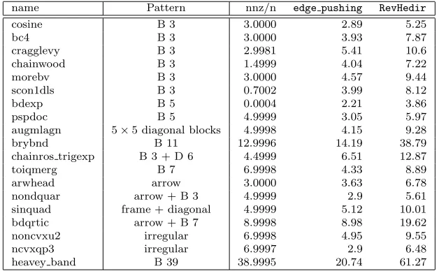
In Table 1, the “Pattern” column indicates the type of sparsity pattern: bandwidth3_{of valuex(Bx), arrow, frame, number of diagonals (Dx), or}

irreg-ular pattern. The “nnz/n” column gives the number of nonzeros in D3_f(x).d

over the dimensionn, which serves as a of measure density. For each problem, we appliedRevHedirand edge pushingAlgorithm 11 and 10 to the objective function f : Rn _{→ R, with x}

i =i and di = 1, for i = 1, . . . , n, and give the

runtime of each method for dimensionn= 106_{in Table 1. Note that all of these}

matrices are very sparse, partly due to the “thinning out” caused by the high order differentiation. This probably contributed to the relatively low runtime, for in these tests, the run-times have a 0.75 correlation with the density measure “nnz/n”. This leads us to believe that the actual pattern is not a decisive factor in runtime.

We did not benchmark our results against an alternative algorithm for we could not find a known AD package that is capable of efficiently calculating such directional derivatives for such high dimensions. For small dimensions, we used the tensor eval of ADOL-C to calculate the entire tensor using univariate forward Taylor series propagation[12]. Then we contract the resulting tensor with the vectord. This was useful to check that our implementation was correct, though it would struggle with dimensions overn= 100, thus not an appropriate comparison.

A remarkable feature of these tests, is that the time spent byRevHedirto calculate D3_{f(x)·d was, on average, 108% that of calculatingD}2_{f(x). Thus,}

2_{As checked May 28th, 2013} 3_{The bandwidth of matrix M = (m}

ij) is the maximum value of 2|i−j|+ 1 such that

name Pattern nnz/n edge pushing RevHedir

cosine B 3 3.0000 2.89 5.25

bc4 B 3 3.0000 3.93 7.87

cragglevy B 3 2.9981 5.41 10.6

chainwood B 3 1.4999 4.04 7.22

morebv B 3 3.0000 4.57 9.44

scon1dls B 3 0.7002 3.99 8.12

bdexp B 5 0.0004 2.21 3.86

pspdoc B 5 4.9999 3.05 5.97

augmlagn 5×5 diagonal blocks 4.9998 4.15 9.28

brybnd B 11 12.9996 14.19 38.79

chainros trigexp B 3 + D 6 4.4999 6.51 12.87

toiqmerg B 7 6.9998 4.33 8.89

arwhead arrow 3.0000 3.63 6.78

nondquar arrow + B 3 4.9999 2.9 5.61

sinquad frame + diagonal 4.9999 5.12 10.01

bdqrtic arrow + B 7 8.9998 8.98 19.62

noncvxu2 irregular 6.9998 4.95 9.55

ncvxqp3 irregular 6.9997 2.9 6.48

heavey band B 39 38.9995 20.74 61.27

Table 1: Description of problem set together with the execution time in seconds of edge pushandRevHedirforn= 106_.

if the user is prepared to pay the price for calculating the Hessian, he could also gain some third order information for approximately the same cost. The code for these tests can be downloaded from the Edinburgh Research Group in Optimization website: http://www.maths.ed.ac.uk/ERGO/.

5

Conclusion

Our contribution boils down to a framework for designing high order reverse methods, and an efficient implementation of the directional derivative of the Hessian calledRevHedir. The framework paves the way to obtaining a reverse method for all orders once and for all. Such an achievement could cause a paradigm shift in numerical method design, wherein, instead of increasing the number of steps or the mesh size, increasing the order of local approximations becomes conceivable. We have also shed light on existing AD methods, providing a concise proof of the edge pushing [8] and the reverse gradient directional derivative [1] algorithms.

The novel algorithms 5 and 6 for calculating the third-order derivative and its contraction with a vector, respectively, fulfils what we set out to achieve: they accumulate the desired derivative “as a whole”, thus taking advantage of overlapping calculations amongst individual components. This is in contrast with what is currently being used, e.g., univariate Taylor expansions [12] and repeated tangent/adjoint operations [18]. These algorithms can also make use of the symmetry, as illustrated in our implementation of RevHedirAlgorithm 11, wherein all operations are only carried out on a lower triangular matrix.

We implemented and tested theRevHedirwith two noteworthy results. The first is its capacity to solve sparse problems of large dimension of up to a million variables. The second is how the time spent byRevHedirto calculate the direc-tional derivativeD3_{f(x)·dwas very similar to that spent by edge pushingto}

this in future work through complexity analysis. Should this be confirmed, it would have an immediate consequence in the context of nonlinear optimization, in that the third-order Halley-Chebyshev methods could be used to solve large dimensional problems with an iteration cost proportional to that of Newton step. In more detail, at each step the Halley-Chebyshev methods require the Hessian matrix and its directional derivative. The descent direction is then calculated by solving the Newton system, and an additional system with the same sparsity pattern as the Newton system. If it is confirmed that solving these systems costs the same, in terms of complexity, then the cost of a Halley-Chebyshev iteration will be proportional to that of a Newton step. Though this comparison only holds if one uses these automatic differentiation procedures to calculate the derivatives in both methods.

The CUTE functions used to test both edge pushing and RevHedir are rather limited, and further tests on real-world problems should be carried out. Also, complexity bounds need to be developed for both algorithms.

A current limitation of reverse AD procedures, such as the ones we have presented, is their issue with memory usage. All floating point values of the intermediate variables must be recorded on a forward sweep and kept for use in the reverse sweep. This can be a very substantial amount of memory, and can be prohibitive for large-scale functions [21]. As an example, when we used dimensions of n = 107_{, most of our above test cases exhausted the available}

memory on the personal laptop used. A possible solution to this, is to allow a trade off between run-time and memory usage by reversing only parts of the procedure at a time. This method is called checkpointing [21, 20].

References

[1] J. Abate, C. Bischof, L. Roh, and A. Carle,Algorithms and design

for a second-order automatic differentiation module, in Proceedings of the

1997 International Symposium on Symbolic and Agebraic Computation, New York, 1997, ACM, pp. 149–155.

[2] I. Bongartz, A. R. Conn, N. Gould, and P. L. Toint, CUTE:

constrained and unconstrained testing environment, ACM Transactions on

Mathematical Software, 21 (1995), pp. 123–160.

[3] B. Christianson, Automatic Hessians by reverse accumulation, IMA Journal of Numerical Analysis, 12 (1992), pp. 135–150.

[4] G. F. Corliss, A. Griewank, and P. Henneberger, High-order stiff

ODE solvers via automatic differentiation and rational prediction, in

Lec-ture Notes in Computer Science, Springer, 1997, pp. 114–125.

[5] L. E. Fraenkel, Formulae for high derivatives of composite functions, Mathematical Proceedings of the Cambridge Philosophical Society, 83 (2008), p. 159.

[6] A. H. Gebremedhin, F. Manne, and A. Pothen,What color is your

Jacobian? Graph coloring for computing derivatives, SIAM Review, 47

[7] A. H. Gebremedhin, A. Tarafdar, A. Pothen, and A. Walther,

Efficient computation of sparse Hessians using coloring and automatic

dif-ferentiation, INFORMS Journal on Computing, 21 (2009), pp. 209–223.

[8] R. M. Gower and M. P. Mello,A new framework for the computation

of Hessians, Optimization Methods and Software, 27 (2012), pp. 251–273.

[9] A. Griewank, D. Juedes, and J. Utke, ADOL-C, a package for the

automatic differentiation of algorithms written in C/C++, ACM

Transac-tions on Mathematical Software, 22 (1996), pp. 131–167.

[10] A. Griewank and U. Naumann, Accumulating Jacobians as chained

sparse matrix products, Mathematical Programming, 95 (2003), pp. 555–

571.

[11] A. Griewank and A. Walther, Evaluating derivatives, Society for Industrial and Applied Mathematics (SIAM), Philadelphia, PA, second edi ed., 2008.

[12] A. Griewank, A. Walther, and J. Utke,Evaluating higher derivative

tensors by forward propagation of univariate Taylor series, Mathematics of

Computation, 69 (2000), pp. 1117–1130.

[13] J. Guckenheimer and B. Meloon,Computing periodic orbits and their

bifurcations with automatic differentiation, SIAM Journal on Scientific

Computing, 22 (2000), pp. 951–985.

[14] J. Guti´errez and M. Hern´andez, A family of Chebyshev-Halley type

methods in Banach spaces, Bulletin of the Australian Mathematical Society,

55 (1997), p. 113.

[15] W. Hock and K. Schittkowski, Test examples for nonlinear

program-ming codes, Journal of Optimization Theory and Applications, 30 (1980),

pp. 127–129.

[16] V. Kariwala, Automatic Differentiation-Based Quadrature Method of

Moments for Solving Population Balance Equations, AIChE Journal, 58

(2012), pp. 842–854.

[17] Ladislav Luksan Jan Vlcek,Test problems for unconstrained optimiza-tion, Tech. Report 897, Academy of Sciences of the Czech Republic, 2003. [18] U. Naumann,The Art of Differentiating Computer Programs: An

Intro-duction to Algorithmic Differentiation, no. 24 in Software, Environments,

and Tools, SIAM, Philadelphia, PA, 2012.

[19] R. D. Neidinger, An Efficient Method for the Numerical Evaluation of

Partial Derivatives of Arbitrary Order, ACM Transactions on

Mathemati-cal Software, 18 (1992), pp. 159–173.

[20] J. Sternberg and A. Griewank, Reduction of Storage Requirement by

Checkpointing for Time-Dependent Optimal Control Problems in ODEs,

[21] A. Walther and A. Griewank, Advantages of Binomial

Checkpoint-ing for Memory-reduced Adjoint Calculations, Numerical Mathematics and