Machines:Generating UIO Sequences
.
White Rose Research Online URL for this paper:
http://eprints.whiterose.ac.uk/147597/
Version: Accepted Version
Article:
Hierons, R.M. orcid.org/0000-0002-4771-1446 and Turker, U.C. (2016) Parallel Algorithms
for Testing Finite State Machines:Generating UIO Sequences. IEEE Transactions on
Software Engineering, 42 (11). pp. 1077-1091. ISSN 0098-5589
https://doi.org/10.1109/tse.2016.2539964
© 2016 IEEE. Personal use of this material is permitted. Permission from IEEE must be
obtained for all other users, including reprinting/ republishing this material for advertising or
promotional purposes, creating new collective works for resale or redistribution to servers
or lists, or reuse of any copyrighted components of this work in other works. Reproduced
in accordance with the publisher's self-archiving policy.
[email protected] https://eprints.whiterose.ac.uk/
Reuse
Items deposited in White Rose Research Online are protected by copyright, with all rights reserved unless indicated otherwise. They may be downloaded and/or printed for private study, or other acts as permitted by national copyright laws. The publisher or other rights holders may allow further reproduction and re-use of the full text version. This is indicated by the licence information on the White Rose Research Online record for the item.
Takedown
If you consider content in White Rose Research Online to be in breach of UK law, please notify us by
Parallel Algorithms for Testing Finite State
Machines:
Generating UIO sequences
Robert M. Hierons,
Senior Member, IEEE
and Uraz Cengiz T ¨urker
Abstract—This paper describes an efficient parallel algorithm that uses many-core GPUs for automatically deriving Unique Input Output sequences (UIOs) from Finite State Machines. The proposed algorithm uses the global scope of the GPU’s global memory through coalesced memory access and minimises the transfer between CPU and GPU memory. The results of experiments indicate that the proposed method yields considerably better results compared to a single core UIO construction algorithm. Our algorithm is scalable and when multiple GPUs are added into the system the approach can handle FSMs whose size is larger than the memory available on a single GPU.
Index Terms—Software engineering/software/program verification, software engineering/testing and debugging, Software engineer-ing/test design, Finite State Machine, Unique Input Output Sequence generation, General Purpose Graphics Processing Units.
F
1
INTRODUCTION
S
OFTWAREtesting is an important part of the softwaredevelopment process but is typically expensive, man-ual and error prone. This has led to significant interest in automation and one of the most promising approaches
is model-based testing (MBT) in which test automation
is based on a model of the system under test (SUT) or some aspect of the SUT. Many MBT methods base test automation on afinite state machine(FSM), with this line of work going back to Moore’s seminal paper [1].
Many FSM-based test generation methods check that the transitions of the FSM specification M have been implemented correctly. In order to check a transition it is necessary to have some method that checks that the state of the SUT, after inputxin states, is the expected state
s′
. This is typically achieved by using input sequences that distinguish the states ofM. Ideally, one has a distin-guishing sequence (an input sequence that distinguishes all of the states ofM) and early work by Hennie showed how a test sequence can be automatically derived when there is a known distinguishing sequence [2]. However, an FSM need not have a distinguishing sequence and instead one might use a unique input output sequence (UIO) for a states′: an input sequence that distinguishes s′from all other states ofM but need not distinguish any
other pairs of states ofM. Although not all FSMs have a UIO for each state, it has been reported that in practice most FSMs do have such UIOs [3] and this has led to the development of many FSM-based test generation methods that use UIOs [3], [4], [5], [6], [7], [8], [9], [10], [11]. However, it is known that the problem of checking
• Department of Computer Science, Brunel University London, UK. E-mail:{rob.hierons,uraz.turker}@brunel.ac.uk
of a standard CPU. Despite their limited instruction sets, the performance of GPUs make them highly effective when used to solve certain types of problems. In addi-tion, the demand for high performance graphics (due to computer gaming, high resolution image processing and big data research) led to increasing parallelism. In fact, new massively parallel computing processors such as the NVIDIA’s Tesla-K40 already have 2880 cores where a core has clock speed of 745 MHz, 288 GB/sec memory bandwidth, and 12 GB of memory.
The constraints imposed by GPU computing led to us devising an algorithm that is entirely new with the exception of the fact that it utilises the ‘Unique Prede-cessor’ approach devised by Naik [15]. Otherwise the proposed algorithm is unique since all the existing brute force approaches in the FSM based literature construct a ‘UIO Tree’ and this is not appropriate due to the space/time limitations (as shown by the experiments). There were several additional challenges related to mem-ory management. These challenges include the need to efficiently distribute data processing between the CPU and GPU, thread synchronisation, optimisation of data transfer, and the capacity constraints of GPU memory.
This paper proposes a massively parallel UIO (P-UIO) generation algorithm that addresses these problems in the context of deriving UIOs for a deterministic com-pletely specified FSM. The P-UIO algorithm was evalu-ated against Naik’s algorithm using randomly generevalu-ated FSMs with up to 1,048,576 states. In the experiments the proposed algorithm constructed UIOs significantly faster (by a factor of 11000 on average) and for much larger FSMs (by a factor of 512). For example, the P-UIO algorithm was able to handle FSMs with 1,048,576 states in under 2 seconds on average while the implementation of Naik’s algorithm took 1231 seconds on average for FSMs with 2048 states. We also performed experiments on some much smaller benchmark FSMs, with between 4 and 48 states. The performance of the two algorithms was similar for these FSMs but the P-UIO algorithm took less time to find UIOs for the larger benchmark FSMs. Unsurprisingly, the differences in performance were less significant for the (much smaller) benchmark FSMs.
This paper is organised as follows. Section 2 intro-duces the terminology used and reviews previously de-vised UIO generation techniques. Section 3 provides an overview of the proposed parallel UIO algorithm and de-scribes the high-level design. Section 4 provides the low-level design. In Section 5 we describe the experiments designed to evaluate the proposed UIO construction algorithm and the results of these experiments. Finally, in Section 6 we provide concluding remarks and discuss possible lines of future work.
2
PRELIMINARIES
2.1 Finite State Machines (FSMs)
A finite state machine (FSM) M is defined by a
tu-ple (S, X, Y, δ, λ) where S is a finite set of states,
X = {x1, x2, . . . , xp} is a finite set of inputs, Y =
{o1, o2, . . . , or}is a finite set of outputs,δis the transition function of type δ : S ×X → S and λ is the output function of type λ : S ×X → Y. The functions δ and
λ are total functions and so M is completely-specified. If FSM M is in state s ∈ S and input x ∈ X is applied then M moves to the state s′ = δ(s, x) and produces
output o = λ(s, x). Such a transition will be denoted
τ = (s, x/o, s′) and we say that x/o is the label of τ
(label(τ)),s is thestart stateofτ (start(τ)), and s′ is the
end stateofτ(end(τ)). Note that sometimes the definition
of an FSM includes an initial state; we do not include this since we are interested in distinguishing states of an FSM and so do not require there to be an initial state.
We use juxtaposition to denote concatenation: if x1,
x2, and x3 are inputs then x1x2x3 is an input sequence.
Given a setX we letX∗denote the set of finite sequences
of elements ofX and letXk denote the set of sequences inX∗that have lengthk. The symbolεis used to denote
the empty sequence.
An input/output sequence consists of a sequence of input/output pairs of the form x1/o1 x2/o2. . . xm/om. We will also write x1x2. . . xm/o1o2. . . omto denote this input/output sequence, where x1x2. . . xm is called the
input portion and o1o2. . . om is called the output portion
of the input/output sequence. ApathinM is a sequence of transitions τ¯ = τ1τ2. . . τm such that start(τi) =
end(τi−1), for all 1 < i ≤ m. The label of a path is
an input/output sequence which is the concatenation of the labels (input/output pairs) of the transitions in that path. For path ¯τ=τ1τ2. . . τm, we define label(¯τ) =
label(τ1)label(τ2). . . label(τm).
The transition and output functions can be extended to input sequences as follows. For x¯ ∈ X⋆ and x ∈X,
¯
δ(s, ε) =s, ¯δ(s, xx¯) = ¯δ(δ(s, x),x¯),λ¯(s, ε) =ε,λ¯(s, xx¯) =
λ(s, x)¯λ(δ(s, x),x¯). We call a subset B ⊆ S of states a
group. The transition and output functions are extended
to groups as follows. For a group B and x¯ ∈ X⋆,
¯
δ(B,x¯) =∪s∈B{δ¯(s,x¯)}andλ¯(B,x¯) =∪s∈B{λ¯(s,x¯)}. We will useδ andλto denote δ¯and λ¯, respectively.
An input sequence x¯∈X⋆ is asplitting sequencefor a groupB, if|λ(B,x¯)|>1. Such an input sequence¯xleads to different output sequences from at least two states in
B and sox¯ splits B. We call an input xa splitting input forB ifxis a splitting sequence of length one forB. If for every pair of states of FSMM there exists a splitting sequence thenM is said to beminimal.
In this work, we consider only deterministic, completely-specified, minimal FSMs. An FSM can be minimised in polynomial time [22]. Further, an FSM that is not completely-specified can often be completed by adding either an error state or transitions with null output1. Thus, the main restriction is that we only
con-sider deterministic FSMs. While non-determinism can be a useful abstraction technique, and some classes of
s
1
s
2
s
3
s
4
x
1
/
o
2
x
2
/
o
1
x
1
/
o
1
x
2
/
o
1
x
1
/
o
1
,
x
2
/
o
1
x
1
/
o
1
[image:4.612.80.266.57.230.2]x
2
/
o
1
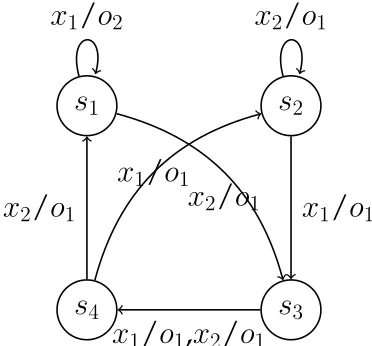
Figure 1: An example deterministic, completely specified and minimal FSMM1.
systems are non-deterministic, the main focus of FSM-based testing work has been on deterministic FSMs and these have been found to be sufficient in important application domains such as hardware [24], protocol conformance testing [5], [25], [26], [27], [28], [29], object-oriented systems [30], web services [31], [32], [33], [34], and general software [35].
An FSM M can be represented by using a directed graphGwhere the vertices ofGcorrespond to the states of M and the edges of G correspond to the transitions ofM. An FSMM isstrongly connectedif the correspond-ing directed graph G is strongly connected (for any ordered pair (v, v′) of vertices there is a path from v
to v′). In Figure 1 an example FSM M
1 is given, where
S = {s1, s2, s3, s4}, X = {x1, x2}, and Y = {o1, o2}.
It is straightforward to see that this FSM is strongly connected. Note that M1 is a minimal machine, since
the input sequencex1x2x1x1x2x1 is a splitting sequence
for every pair of different states.
For a given FSM, state verification can be achieved by using a Distinguishing sequence (DS),unique input/output
sequences (UIOs), aCharacterising set (CS), or state
identi-fiers. A distinguishing sequence is an input sequencex¯
such that for every pair (s, s′) of distinct states of FSM M,M produces different output sequences in response tox¯ fromsand s′
(λ(s,x¯)6=λ(s′
,x¯)). Unfortunately, not all FSMs have a DS. An alternative is to use anadaptive
distinguishing sequence, which is an adaptive process that
determines the next input to apply on the basis of the output observed. Since ADSs generalise DSs, an FSM that has a DS also has an ADS and an additional benefit is that it is possible to determine whether an FSM has an ADS in low-order polynomial time [36].
A UIO for state s is an input/output sequence x/¯ ¯o
such that λ(s,x¯) = ¯o and for all s′ ∈ S\ {s}, we have
that λ(s′
,x¯)6= ¯o. While not every FSM has UIOs for all states, some FSMs without a DS or ADS have UIOs for all states. There may be value in using UIOs even when
an FSM has a DS since the UIOs may be shorter than the DS. For example, states1ofM1 has a UIO (x1/o2) of
length1 but it is straightforward to check thatM1 does
not have a DS of length1. It has also been found that in practice many FSMs have UIOs for all states [3].
A characterising set (CS) is a setW of input sequences that can distinguish any pair of states. A minimal FSM with nstates has a CS with at most n−1 sequences of length at mostn−1and such a CS can be found in poly-nomial time. If every sequence in W is executed from state s, the set of output sequences identifies/verifies
s. However, the use of characterising sets could lead to long test sequences [37]. In addition, most test generation techniques that use a characterising set return many test sequences and it has been noted that the process of resetting a system between test sequences can be expensive [38], [39], [40], [41]. As a result, it is desirable to use a DS or UIOs where they exist (and are sufficiently short) and use a characterising set otherwise. Since the size of a characterising set is of O(n2
), it has been suggested that if a UIO or DS is longer than an O(n2
)
upper bound then it might be best to use a characterising set. This has led to the suggestion that one might initially attempt to find a DS or UIOs but only use a DS/UIOs if the length is lower that the given bound. There has been much interest in UIOs [42], [43] since they help in state transition fault detection and have been found to yield shorter test sequences than using the DSs and CSs [42], [43].
It has been observed that it may not be necessary to use all of the sequences from a characterising set in order to identify a state s of the FSM [44]. This has led to the notion of state identifiers, where a state identifier (or separating set) for statesis a set of input sequences that distinguishsfrom all other states of the FSMM. The use of state identifiers can lead to smaller test suites, when compared to characterising sets.
2.2 Previous UIO generation methods and Inference Rules
Since UIOs have been used in automated FSM-based test generation methods, there has been interest in the problem of devising UIOs. Although the problem of checking the existence of UIOs is PSPACE-Complete [36], the value of UIOs in test generation has led to significant interest in UIO generation.
It is possible to represent UIO generation in terms of a UIO tree (Definition 2.1) [15].
Definition 2.1: Let M be an FSM with set of states S
(|S|=n). AUnique Input Output TreeforSis a rooted tree
T such that nodes are labeled with two groups (initial group I and current group C) and edges are labeled with input/output pairs. A node of T is called a leaf node if its groups have cardinality one. If two distinct edges leaving a nodev share the same input label then these edges have different output labels. For every node
I={s1, s2, s3, s4}
C={s1, s2, s3, s4}
I={s1, s2, s3, s4}
C={s3, s2, s4, s1}
. . .
. . . x2/o1
I={s4} C={s1} x1/o2
. . . x1/o1
x2/o1
I={s4} C={s1} x1/o2
. . .
. . . . . . / . . .
. . . . . . / . . .
x1/o1
x2/o1
I={s1}
C={s1}
x1/o2
I={s2, s3, s4}
C={s3, s4, s2}
I={s2, s3, s4} C={s4, s2, s3}
. . . .
x1/o1
I={s2, s3, s4} C={s4, s1, s2}
I={s2, s3} C={s2, s3} x1/o1
I={s4} C={s1} x1/o2
I={s2, s3, s4} C={s1, s3, s2} x2/o1
x2/o1
x1/o1
[image:5.612.363.496.55.174.2]... ... ... ... ... ... ... ... ... ... ... ... ℓ
Figure 2: An example of a UIO Tree of depthℓfor FSM
M1 given in Figure 1.
concatenating the edge labels on the path from the root node to v, then we have that I = {s ∈ S|λ(s,x¯) = ¯o}
andC=∪s∈I{δ(s,x¯)}. A UIO tree iscompleteif for every statesithere exists a leaf nodevwith initial setI={si}.
An example UIO tree forM1 is given in Figure 2.
As the upper bound on UIO length is exponential, the process of constructing UIO trees from scratch can be expensive. This led to Naik [15] proposing an approach to construct UIOs in which inference rules are used. In this method some minimal length UIOs are found and these UIOs are used to deduce UIOs for other states. The inference rules operate as follows: If x/¯ o¯ is a UIO for state s and τ = (s′
, x/o, s) is the only transition
that reaches states with label x/o, thenxx/o¯ o¯is a UIO for s′
. Here state s′
is known as a unique predecessor of state s. Note that the notion of ‘unique’ here is for the state and input/output; there might be more than one unique predecessor for a state s. Since a machineM is assumed to be strongly connected, it may be possible to use inference rules to compute UIO sequences for all states once we have constructed only a few UIOs. In order to achieve this we have a database, called a rule base, containing the known inference rules for the FSM. In the following, we formalise what it means for a state to be a unique predecessor.
Definition 2.2: For state s∈S,s′∈S
is aunique
prede-cessorforsif there exists a transitionτwithstart(τ) =s′
,
end(τ) = sand label(τ) = x/o such that there exists no
transitionτ′6=τ with end(τ) =sand label(τ) =x/o.
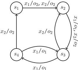
As an example, see the FSMM2in Figure 3a. Note that
for state s1 the unique predecessor iss4 with transition
labeled byx2/o2, for states4the unique predecessor iss3
with transition labeled by x1/o1, for state s3the unique
predecessor is s2 with transition labeled by x2/o2 and
finally for state s2 the unique predecessor is s1 with
transition labeled by x1/o2. The rule base table for FSM
M2 is given in Figure 3b. Let us assume that by using a
UIO tree we can construct a UIO for state s1. Then by
using the rule base table, we can derive UIOs for all of the states of the FSM (Figure 3c).
If an FSM does not possess UIOs for all of its states, the inference rules do not solve the problem. Naik’s
al-s1 s2
s3
s4
x1/o2,x2/o2
x
1/
o
1,
x
2/
o
2
x1/o1
x2/o2
x1/o1
x2/o2
(a) A deterministic, completely specified and
minimal FSMM2
State unique predecessor τ
s1 s4 x2/o2
s2 s1 x1/o2
s3 s2 x2/o2
s4 s3 x1/o1
(b) Rule base (rb) table for FSMM2given in
Figure 3a
State U IO
s1 x
1/o2
s2 x2x1x2x1/o2o1o2o2
s3 x1x2x1/o1o2o2
s4 x2x1/o2o2
(c) Assume that UIO for states1is computed
[image:5.612.356.536.81.406.2]throught a UIO tree (bold typed). Then by using the rule base table given in Figure 3b we can derive UIOs for other states.
Figure 3: An FSM M2 with its rule base. After the UIO
for s1 is computed, UIOs for every other state can be
obtained by using the rule base.
gorithm then constructs the full UIO tree, which requires exponential time/space.
2.3 The CUDA Programming Model
Compute Unified Device Architecture (CUDA) is NVIDIA’s parallel computing architecture that combines software and hardware architectures. We first present an overview of the CUDA hardware model.
From the programmer’s point of view the CUDA model is a collection of threads running in parallel, with a collection of threads, called a warp, running simultaneously on a multiprocessor. The warp size can vary according to the GPU. The programmer decides on the number of threads to be executed. If the number of threads is more than the warp size then these threads are time-shared internally on the multiprocessor. At a given time, a block of threads runs on a multiprocessor. The maximum number of threads in a block can vary according to the underlying GPU. However, multiple blocks can be assigned to a single multiprocessor and their execution is again time-shared. The collection of blocks for a single program is called a grid and the maximum number of grids can vary according to the GPU.
All threads of all blocks executing on a single mul-tiprocessor divide its resources equally amongst them-selves. Each thread executes a piece of code called a
kernel. The kernel is the core code to be executed on
a multiprocessor. Upon execution, thread ti is given a unique ID and during execution thread ti can access data residing in the GPU by using its ID. Since the GPU memory is available to all the threads, a thread can access any memory location. This allows programmers to interpret a device as a Parallel Random Access Machine (PRAM) architecture through the usage of global device memory. However, the performance improves with the use of shared memory (which can only be accessed by threads within a block), as such memory can be accessed faster than the global device memory. During GPU computation the CPU can continue to operate. Therefore the CUDA programming model is a hybrid computing model in which a GPU is referred as a co-processor (device) for the CPU (host).
3
HIGH-LEVEL DESIGN
In this section we present the high-level design of the proposed massively parallel (P-UIO) algorithm for deriv-ing UIOs from FSMs. We start by discussderiv-ing the design decisions made in developing the P-UIO algorithm and then provide an overview of the P-UIO algorithm. In Section 4 we provide additional information regarding the data structures used.
3.1 Parallel design: From UIO-Tree to Sorting
In the proposed parallel algorithm, we aimed to address several bottlenecks that we may encounter while using na¨ıve UIO tree construction algorithms.
1) Sequential process: A na¨ıve sequential UIO tree generation algorithm iterates over a UIO tree T
and would process this tree node-by-node. Here each node is associated with a group and the same input is applied to each state in a group (since these states have yet to be distinguished). (Figure 4).
s1, s2, . . . , sn
si, sj, . . . , sm sk, sl, . . . , sn
CURRENT GROUP
(a) Sequential algorithm selects a group during execution stepi.
s1, s2, . . . , sn
si, sj, . . . , sm sk, sl, . . . , sn
getδ(si, x)
(b) Sequential algorithm se-lects a state during execu-tion stepi.
s1, s2, . . . , sn
si, sj, . . . , sm sk, sl, . . . , sn
getδ(sj, x)
(c) Sequential algorithm se-lects another state during execution stepi+ 1.
s1, s2, . . . , sn
si, sj, . . . , sm sk, sl, . . . , sn
[image:6.612.328.552.62.248.2]CURRENT GROUP (d) Sequential algorithm se-lects another group during execution stepi+ (m).
Figure 4: Steps of sequential algorithm overview. Note only current states are illustrated.
s1, s2, . . . , sn
si, sj, . . . , sm sk, sl, . . . , sn
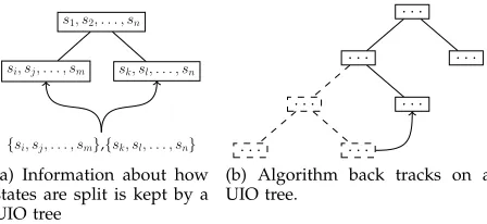
{si, sj, . . . , sm},{sk, sl, . . . , sn}
(a) Information about how states are split is kept by a UIO tree
. . .
. . .
. . .
. . . .
. . . . . .
(b) Algorithm back tracks on a UIO tree.
Figure 5: Use of tree structure while constructing a UIO-tree. Note only current states are illustrated.
2) Memory Requirements: During UIO tree computa-tion, all portions of the UIO tree would be kept in memory since:
• It includes information about how the states are
split (Figure 5a) and
• It makes it possible to back-track when
re-quired (Figure 5b).
In developing a massively parallel approach, one might construct a UIO-tree and choose to have a threadti process a single node of a UIO-tree. The threadtiwould process all of the data associated with a node [12], [15] (Figures 7a). However, a node can have many current and initial states and for an FSM with nstates, a node is associated with data whose size is ofO(n). Although the maximum number of states associated with a node reduces as the depth of the tree increases, the rate at which this happens will vary between FSMs (Figure 7b). As a result, an approach that directly represents the UIO tree may not scale well for very large FSMs.
[image:6.612.326.550.298.401.2]can be achieved.
s1 s2 s3 s4 s5 . . . sn
o2 o2 o1 o3 o3 . . . o2
o1 o1 o1 o2 o1 . . . o2
..
. ... ... ... ... ... o1
o1 o2 o1 o2 o2 . . . o1
(a) Output sequences
s3 s9 s1 s7 s11 . . . s4
o1 o1 o2 o2 o2 . . . o3
o1 o1 o1 o2 o2 . . . o3
..
. ... ... ... ... ... o3
o1 o1 o1 o1 o1 . . . o3
= 6=
6
= =
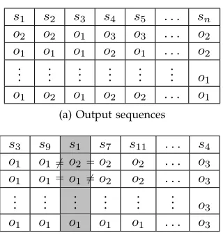
[image:7.612.94.254.71.240.2](b) Revealing distinguished states by consider-ing sorted output sequences
Figure 6: The use of sorting while finding distinguished states.
Consider Figure 6a, which gives output sequences pro-duced by thenstates of an FSM in response to an input sequence x¯. Input sequence x¯ uniquely distinguishes a state if and only if the output sequence produced by this state is unique. Thus, we can use an approach that finds columns in which the output sequences are unique. We can re-formalise this problem as follows: We are given a set of sequences of the same length and want to find the
different sequences. This problem can be solved by sorting
the output sequences: after sorting, if the column being considered is different from its neighbouring columns then it is unique (Figure 6b). A benefit of this is that sort-ing can be parallelised and can be efficiently performed by GPUs [19]. Thus, in the P-UIO algorithm we used an approach based on sorting in order to determine which states have been distinguished.
In order to be able to use sorting we need to intro-duce an alternative formalisation for constructing UIO sequences. Rather than represent the problem in terms of UIO-trees, we use what we call input output vectors; later we will see how we can base a scalable parallel UIO generation algorithm on this formalisation.
. . .
. . .
. . . .
. . .
. . . . ti
tj tk
tl tm tn to
(a) Each thread processes a node of a tree concurrently.
. . . .
. . . .
. . . .
. . . . .
.
(b) An unbalanced UIO tree with very large groups.
Figure 7: Different views for parallelism (a),(b) on a UIO tree and an illustration for an unbalanced UIO-tree (c).
Definition 3.1: An input/output vector (IO-vector) V
for an FSM M = (S, X, Y, δ, λ) with n states is a vector with n elements such that: For statesi ∈ S there exists an element v in V that is associated with initial state
si, a current state sc ∈ S, an input sequence X¯(v) such
thatδ(si,X¯(v)) =sc, and an output sequence O¯(v)such thatλ(si,X¯(v)) = ¯O(v). We will say that an IO-vector is
homogeneousif every pair of elements that have the same
output sequence also have the same current state. We are interested in whether an IO-vector is homoge-nous since there is no value in extending such an IO-vector with further input: if two initial states s and s′
have not been distinguished in this IO-vector (they have the same output sequences) then they are mapped to the same current state and so cannot be distinguished by further input. Thus, whenever the search for UIOs finds a homogenous IO-vector it will back-track.
In UIO generation, we will ‘evolve’ the elements of an IO-vector and will do so in a manner that is consistent with the notion of a UIO. We sort the output sequences to determine whether the states corresponding to two elements have been distinguished: two elements share the same output sequence if they have not been distin-guished. In each iteration, for each output sequence that appears in the current IO-vector the algorithm chooses a next input to use. Let us suppose that element v is associated with initial statesiand current statesc. If the next input to apply in v isx then v is said toevolve to a new elementv′
with inputx (evolve(v) = (x, v′
)) and we have thatv′
is associated with initial statesi, current states′
c, input and output sequencesX¯(si)x/O¯(si)osuch thatδ(sc, x) =sc′ and λ(sc, x) =o. The P-UIO algorithm will ensure that given an IO-vector V, if elements v
andv′
have the same associated input/output sequence then the process of evolving V will lead to the same next inputs in v and v′. As a result, for any pair of
elementsvandv′ such thatO¯(v) = ¯O(v′)we have that: if evolve(v) = (x, v′′)andevolve(v′) = (x′, v′′′)then x=x′.
The following shows how IO-vectors are related to UIOs.
Lemma 3.1: Let us suppose that V is an IO-vector for
M and thatV has an elementvwhose initial state iss. If there does not exist v′
∈V \ {v}such that O¯(v) = ¯O(v′
)
then X¯(v)is a UIO fors.
The proposed algorithm iterates over an IO-vector and ideally obtains what is called a UIO-vector.
Definition 3.2: An IO-vectorV is said to be aunique
in-put outin-put vector(UIO-vector) if for any pair of elements
v, v′ ∈V
withv6=v′
we have thatO¯(v)6= ¯O(v′)
.
Note that an IO-vector may not evolve into a Uvector. The reason for this is that in evolving an IO-vector the same input is applied to all elements that have the same output sequence. The problem here is that, for example, an FSM might have UIOs for all states but have a pair of statess, s′ such that the UIOs forsands′ start
with different inputs: such a scenario cannot be captured by an IO-vector. Consequently in order to construct UIOs one may need to construct a set of IO-vectors.
[image:7.612.58.291.621.718.2]Thread Vector si,¯x/o¯,sc si,x/¯ ¯o,sc si,x/¯ o¯,sc si,x/¯ ¯o,sc . . .
IO-vectorV si,x/¯ ¯o,sc s′i,x/¯ o¯,s
′
c s
′′
i,x/¯ o¯,s
′′
c s
′′′
i ,x/¯ ¯o,s
′′′
[image:8.612.52.311.52.120.2]c . . .
Figure 8: An illustration for a IO-vector. Each element is associated with an input sequence an initial state, and a current state.
is a full set for FSM M with state setS if for all s∈S,
there exists an IO-vector V′ ∈ V
that has an element v
whose initial state is s and whose input sequenceX¯(v)
is such thatX¯(v)/O¯(v)is a UIO for s.
The following is an immediate consequence of the definition of a full set.
Lemma 3.2: If FSM M has a full set V of IO-vectors
then this defines UIOs for all states of M.
Importantly, an element of an IO-vector contains all information related to the evolution from a single state including the input/output sequence, initial and current states. This representation allows us to have a one-to-one correspondence between threads of the GPU and the elements of an IO-vector (Figure 8), overcoming the issue we had with UIO-trees where if a thread ti processes a node thenti considersO(n)states.
However, note that if we insist on keeping in-put/output sequences within elements then each thread will process a whole input/output sequence during ev-ery iteration. As a result, the memory used by a single thread will increase and this may reduce the scalability of the algorithm. In order to avoid this, we devised an approach in which the input sequence associated with an element is kept elsewhere (not in the element). This is not problematic for inputs: when evolving an IO-vector we do not need to know about the previous inputs. However, we need to determine which elements of an IO-vector must be evolved using the same input. This suggests that threads should consider all the output sequences observed so far.
We addressed this problem as follows. Instead of keeping/sorting all output sequences observed, each element will keep a unique representation of an output sequence, the aim being to reduce the amount of data stored. In order to achieve this, an output sequence ¯o
is represented by an enumeration (enum(¯o)) that assigns a unique representation (number) to o¯. For example, if we reach a point where only two output sequences have been observed then we could simply use the numbers 0
and1. In the next section we describe how enumeration was done.
We will see that one important property of enumera-tion is that the equality relaenumera-tion over strings is preserved.
Lemma 3.3: Given ¯o,o¯′,¯o′′ ∈ Y⋆, enum(¯o)6=enum(¯o′)
if and only if enum(¯oo¯′′)=6 enum(¯o′o¯′′)
. We also have the following results.
Enumerated vector
.. .
00001 00001
00002 00003 .. .
A string vector
.. .
. . . ababbabab. . . . . . ababbabab. . .
. . . abaabbbab. . . . . . aaabbabbb. . .
.. .
[image:8.612.359.512.54.138.2]enum(v[i])
Figure 9: An illustration for enumeration. Each string is compacted to another string. Note that the enum function produces same values when given the same input string (red coloured texts).
vectorV′δ(s, x)δ(s, x)δ(s, x)δ(s, x)δ(s, x). . .
vectorV′′ δ(s, x)δ(s, x)δ(s, x)δ(s, x)δ(s, x). . .
vectorV δ(s, x)δ(s, x)δ(s, x)δ(s, x)δ(s, x). . .
Backtrack δ(s, x)δ(s, x)δ(s, x)δ(s, x)δ(s, x). . .
vectorV δ(s, x)δ(s, x)δ(s, x)δ(s, x)δ(s, x). . .
IDP-d
Homogeneous Vector
× × × × ×
Store, Prepare inputs
Check distinguished states, Use inference Rules, Update enumerations, Decide to back-track/continue
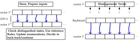
Figure 10: Overview of the steps taken in one iteration of P-UIO algorithm: the algorithm keeps evolving elements through the IDP. Before each iteration the algorithm stores the current data and chooses inputs to be applied. After each IDP, the algorithm checks for distinguished elements, applies inference rules, updates enumerations, and decides to continue or not. If the vector is homoge-neous then it back-tracks.
Lemma 3.4: Let v ∈ V be an element of an IO-vector
associated with initial states. If there does not existv′ ∈ V \ {v} such thatenum( ¯O(v)) =enum( ¯O(v′)) then s is
distinguished from all other states ofM.
Lemma 3.5: Letv and v′ be two elements ofV
associ-ated with initial statess, s′respectively. Ifenum( ¯O(v)) = enum( ¯O(v′)) then s and s′ are not separated and if enum( ¯O(v))6=enum( ¯O(v′))thensand s′ are separated.
We can thus use the enumeration function to reduce the size of the information stored regarding the output sequences observed. It will be possible to define an enumeration function such that the size of the repre-sentation of the output sequence will be no larger than
log(n)since it takeslog(n)space to represent the integers from 0 to n−1 and there can be at most n different output sequences. Further, this information will allow the algorithm to determine which states have not been distinguished in constructing an IO-vector (so must be followed by the same input) using space of size no more thanlog(n)(Figure 9). As a result, the proposed approach will satisfy our requirements regarding GPU memory.
3.2 An overview of the P-UIO algorithm
In this section, we provide an overview of the P-UIO algorithm.
[image:8.612.317.559.207.279.2]the algorithm cannot back-track. The overall algorithm is like a depth-first search that, in an iteration of the main loop, increases the length of the input sequence being considered by d. We could simply increase the input sequence length by1in each iteration; there would then be no need to introduce the parameter d. However, as we will see later, this choice could lead to more frequent (relatively slow) memory transfers between the GPU and CPU to store the current data (for back-tracking).
If the overall depth of the process is greater than or equal to a bound ℓ at the end of an iteration of the main loop then the algorithm back-tracks and stores the elements that are associated with UIOs (those with a unique enumeration of output sequence). Therefore, the algorithm stores UIOs for M when they are found.
The algorithm can return UIOs of length greater than
ℓ ifdis not a factor ofℓ: if kd < ℓ≤(k+ 1)dfor integer
k then the main loop back-tracks if the overall depth reaches(k+1)d. In addition, longer UIOs can be returned if the inference rules are used. The algorithm has the following phases in every iteration of the main loop.
• Phase 1: Apply the iterative deepening process.
– Store the current IO-vector (to allow back-tracking).
– Choose inputs for the next iteration of the deep-ening process. In this work we selected inputs randomly in such a way that no input sequence is applied to an IO-vector twice.
– Apply aniterative deepening process(IDP) on the elements of the IO-vector, increasing the depth byd. The inputs used to evolve elements during the IDP phase are usedin-order. By in-order we mean that elements that are associated with the same output sequences evolve with the same inputs. This ensures that if the same output sequences have been observed from two states
s and s′ then the same next input sequence is
applied. As explained earlier, for reasons of ef-ficiency the algorithm stores (and so compares) enumerations of the output sequences and not the output sequences themselves.
• Phase 2: Gather the outcome of IDP.
– Find elements that define UIOs by sorting; such an element has a unique enumeration (of the output sequence).
– By using inference rules, find additional UIOs.
– Update the representations of output sequences.
• Phase 3: Decide to continue.
– Continue from step 1 if some states do not have known UIOs, the upper bound (ℓ) on UIO lengths has not been reached, and the IO-vector is not homogeneous.
– Backtrack if the upper bound on UIO lengths has been reached and not all UIOs are generated or the vector is homogeneous.
– Terminate if the algorithm has generated a UIO for each state or it is not possible to continue or
back-track.
Figure 10 describes the approach.
For a given state s ∈ S we may need to consider every possible input sequence whose length is below the upper-bound ℓ and so the P-UIO algorithm is an exponential algorithm.
The following is immediate from the definition of the termination condition of the algorithm.
Theorem 3.1: Let us suppose that the P-UIO algorithm
receives an FSM M and inputs d and ℓ. The P-UIO algorithm terminates with success if every state of M
has a UIO sequence of length at mostℓ.
Note that this is not an ‘if and only if’ result since the use ofdand inference rules allows the P-UIO algorithm to return UIOs of length greater thanℓ.
4
LOW-LEVEL DESIGN
In the previous section we provided a high-level overview of the proposed algorithm. However, there is a need to map this to a structure that can be implemented using GPUs. In this section we give these low-level design details of the UIO algorithm. Although the P-UIO algorithm consists of only a few steps, in order to obtain high performance from the GPU, one has to consider the following design principles.
1) Minimise global memory transactions
2) Maximise number of parallel threads per block
3) Prevent thread divergence
Recall that in designing the P-UIO algorithm, our objective is to realise a one-to-one correspondence be-tween the states of the FSM and the threads of the GPU. Therefore, we want to maximise the number of threads used in a block. However, this has implications regarding the use of shared memory on a GPU as shared memory usage limits the number of threads in a block.
Therefore, the P-UIO algorithm we did not use shared memory but instead we tried to minimise the global memory transactions latency. As previously reported [45] global memory transaction latency can be hidden by using (1) many threads and (2) supporting coalesced
memory access in which the threads in a block access
global memory in a manner that allows the GPU to bundle a number of memory accesses into one memory transaction. The principle of memory coalescing is simi-lar to thecache lineprinciple of a CPU, in which a cache line is either completely replaced or not at all. Even if only a single data item is requested, the entire line is read so whenever a neighbouring item is subsequently requested, it is already in the cache.
Type of Memory Data Structure
Texture Memory D F SM,D inf erenceRules
Global Memory D inputs, D outputs,
D statesand temporal vectors.
Registers temporary variables
Local Memory NA
[image:10.612.73.278.52.122.2]Shared Memory NA
Table 1: Summary of the different types of memory used in the P-UIO algorithm.
We now discuss how the high-level P-UIO algorithm was refined for use with GPUs. In order to perform coalesced global memory access, in the P-UIO algorithm we use several structures to represent an IO-vector V; these structures are to be kept in the global memory of the GPU (as opposed to the local memory of a thread) and hold the following information.
1) TheD statesvector holds the relationship between initial and current states: given initial state si,
D states[i]is the corresponding current state.
2) The D inputs vector holds the inputs that will be applied during the next step of IDP.
3) The D outputs vector holds output data: enumer-ations of output sequences observed from initial states. It therefore provides information regarding which states have been distinguished (split). 4) The D F SM vector holds the transitions of the
underlying FSM.
5) D inf erenceRules holds the unique precedence
[image:10.612.310.563.58.358.2]information for each state.
Table 1 summarises the memory management. The FSM and inference rules were associated with the texture memory. The vectors used to construct UIOs (such as
D inputs,D outputs,D states) were declared as global
memory. Variables used for the computation were au-tomatically associated with registers by the compiler. In developing the P-UIO algorithm we did not use local and shared memory.
As explained in Section 3.2, the P-UIO algorithm has a main loop that has three phases:
1) In the first phase IDP is applied to extend the depth by d (Phase 1 in the high-level description of the loop, described in detail in Section 4.1);
2) In the second phase, the outcome of IDP is analysed (Phase 2 in the high-level description, described in detail in Section 4.2); and
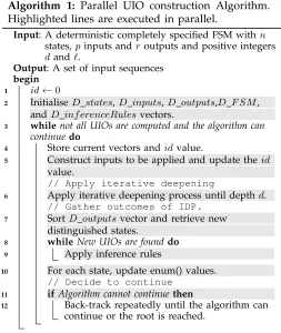
3) In the final phase the algorithm decides whether to continue or back-track (Phase 3 in the high-level description, described in detail in Section 4.3). The algorithm is summarised in Algorithm 1. Here lines 3-5 correspond to Phase 1 in the high-level descrip-tion (Secdescrip-tion 3.2); lines 6-9 correspond to Phase 2; and lines 10-11 correspond to Phase 3. The shading shows the steps that are carried out in parallel.
4.1 Applying the Iterative Deepening Process
Before IDP begins, id and vectors are stored in CPU memory for back-track (Line 4) and then the input vector
Algorithm 1: Parallel UIO construction Algorithm.
Highlighted lines are executed in parallel.
Input: A deterministic completely specified FSM withn states,pinputs androutputs and positive integers dandℓ.
Output: A set of input sequences
begin
1 id←0
2 InitialiseD states,D inputs,D outputs,D F SM, andD inf erenceRulesvectors.
3 whilenot all UIOs are computed and the algorithm can
continuedo
4 Store current vectors andidvalue.
5 Construct inputs to be applied and update theid value.
// Apply iterative deepening
6 Apply iterative deepening process until depthd.
// Gather outcomes of IDP.
7 SortD outputsvector and retrieve new distinguished states.
8 whileNew UIOs are founddo
9 Apply inference rules
10 For each state, update enum() values.
// Decide to continue
11 ifAlgorithm cannot continuethen
12 Back-track repeatedly until the algorithm can continue or the root is reached.
is generated by a parallel random combinator generator (PRCG) (Line 5). This procedure receives an integer value id, number of statesn, alphabet X, the D inputs
vector, and iterative deepening parameterd. PRCG first calls a kernel called random number generator (RNG). RNG receivesn,d, andpand it returns an integer value
υ in the range [0, pnd]. Then the algorithm checks if it can increment2 id, if so the PRCG calls another kernel
(the Fill kernel). The Fill kernel receives υ, X, and the
Dinputs vector as its parameters and fills the D inputs vector with the representation ofυin basep. Otherwise, if the algorithm cannot incrementidthen it calls the RNG kernel and repeats the process. Later the algorithm enters IDP (Line 6).
During an iteration (say the jth iteration) of IDP, the Host calls several kernels one after another. The first kernel to be called is the Apply kernel. During execution of the Apply kernel a thread ti reads the ith value on
D statesvector and gathers the current state. If the value
is−1 the thread halts. Otherwise threadti reads theith value from theDoutputs vector (Doutputs[i]) and retrieves inputx=D inputs[(j∗n) +Doutputs[i]]from theDinputs vector. Note that as an input is computed based on the output, at each iteration the same input is applied to all states for which the values read from the Doutputs vector are identical. Then, the thread uses theD F SM
vector to determine the next state s ∈ S and output
o∈Y. Afterwards, it writes s to the Dstates vector and
2. Note that the algorithm incrementsidifυhas not been selected
it concatenateso withDoutputs[i].
The next step is to update the Doutputs vector. To achieve this, we follow a similar procedure which is applied to check if new pairs of states are split. This procedure is explained in the following section. But in summary we apply two steps: sort the Doutputs vector, write integer values (starting with0) to elements of the
Doutputs vector so that two elements of Doutputs vector are identical if and only if they receive same integer value. As there are at most n different possible output sequences, the number assigned to an element of the
Doutputs vector is between0 andn.
During IDP, for a state si a thread ti will normally read the corresponding indexes on D states,D inputs,
D outputs and D F SM, many times. Although the
reads and writes on theD statesandD outputsvectors are coalesced, transactions on D inputs are not. The index values in the D inputs vector depends on the data retrieved from the D outputs vector. Moreover, since the host can write the FSM transition structure
to D F SM once and the kernels can read this FSM
structure many times, the D F SM vector is stored in the texture memory and so coalescing is not an issue. On the other hand note that IDP does not allow thread divergence. That is, all threads in a warp will process the same instruction of a kernel.
4.2 Gathering outcomes of IDP
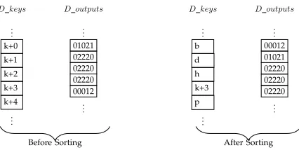
Once IDP ends, we need to check if new pairs of states are split. This is done through a parallel stable sorting (Line 7). The sorting algorithm gathers vectorD outputs
and a vector (D keys) which holds the relative orders of items of D states (the initial state information). It then sorts the states according toD outputs3(Figure 11). The
results of the sort reveals states that are distinguished from all other states (singleton states) and pairs of states that produce the same output sequences.
In order to achieve this a temporary vector (D singletons) is used. After receiving
D keys, D outputs and D singletons a thread (thread
ti) selects a single (ith) item of the D outputs vector and compares the enumeration of the output sequence to those of the neighbouring values (the enumeration of the output sequence read from the i+ 1th and i−1th locations of the D outputs vector). If the ith value is different from both of these values then the thread reads the initial state information from the D keysvector and stores it in theD singletonvector. In order to determine which states are split, another temporary vector called
the D groups vector is used as follows: a thread again
selects a single (ith) item of the D outputs vector and reads the index of the initial state information from the
D keys vector only if one neighbouring output data
is the same as that of the ith item of the D outputs
vector (not both). As a result of this process, for each
3. Note that after the sort, the information inD outputs[i]may not belong to initial statesi.
D outputs
.. . 01021 02220 02220 02220 00012 .. . D keys
.. . k+0|
k+1|
k+2|
k+3|
k+4|
.. .
D outputs
.. . 00012 01021 02220 02220 02220 .. . D keys
.. . b+1|
d+1|
h+1|
k+3|
p+1|
.. .
[image:11.612.332.545.51.158.2]Before Sorting After Sorting
Figure 11: An illustration for sorting. Stable sorting algorithm recives D outputs vector and D keys vector as satellite information.
group of states with the same output data we have two values in the D groups vector indicating the starting and ending indexes of the initial states in a group from
theD keys vector (Figure 12). Note that the process of
finding singletons and groups of states can cause thread divergence, which may prevent threads in a warp from executing concurrently.
After singletons have been found, a kernel uses the inference rules to try to find UIOs for other states (Lines 8–9). In order to achieve this, the ker-nel receives the list of singletons found and the
D Inf erenceRulesvector. Each thread selects one state
from the D singletons vector and finds its unique pre-decessors from theD Inf erenceRulesvector. Note that similar to the D F SM vector, the host can write the
D Inf erenceRulesvector once and the kernels can read
this data many times, therefore the D inf erenceRules
vector is stored in texture memory and so coalesced memory access is not an issue. Moreover, since the algorithm should also consider unique predecessors of fresh states, the kernel may be called by the Host until it reaches a point where no fresh states are found.
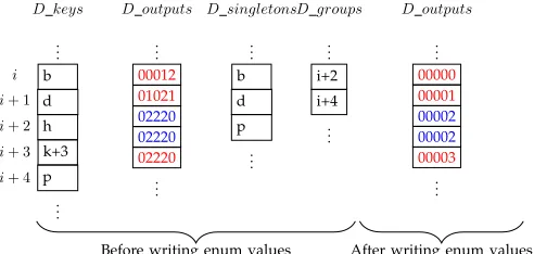
Once singletons and groups have been revealed, the algorithm assigns unique integers (beginning from0) to singleton states and groups of states and this defines the
enumerationof each corresponding output sequence (Line
10). The algorithm then updates representations (i.e.
enum( ¯O(s))) of states. A threadtiis assigned to a group
S′
and generates a unique integer value (κS′ =i). Then
for all s ∈ S′
, ti retrieves the initial state information from theD keys vector and it writes κS′ to D outputs
(Figure 12).
4.3 Checking Termination Conditions
D outputs
.. .
00012 01021 02220 02220 02220
.. .
D keys
.. . b+1|
d+1|
h+1|
k+3|
p+1|
.. .
D singletons
.. . b+1|
d+1|
p+1|
.. .
D groups
.. . i+2|
i+4|
.. .
D outputs
.. .
00000 00001 00002 00002 00003
.. .
i
i+ 1
i+ 2
i+ 3
i+ 4
[image:12.612.52.298.54.171.2]Before writing enum values After writing enum values
Figure 12: An illustration for enumeration. Each string is compacted to another string. Note that for same strings enum function produces same values (red coloured texts).
related to singletons) computed in the current iteration of the main loop is discarded and the previous data, which resides in CPU memory, is brought to GPU memory. The P-UIO algorithm then continues to execute. Otherwise, if a UIO has been found for every state then the algorithm ends execution. If neither of these conditions holds then the algorithm continues to execute with currentD states
and D outputsvectors.
Note that after each IDP the algorithm stores the current data in CPU memory. As memory transactions between CPU and GPU are expensive, it is good practice to reduce the number of such transactions. As a result, it makes sense to select relatively large values ofd. If we pickd= 1then each time we increase the input sequence length by 1 we need to send data back to the CPU and this will reduce the performance of the algorithm. In the next section we report on the results of experiments that show how the value of the parameter d affects the performance of the algorithm.
4.4 Example
We now show the execution of the P-UIO algorithm using an example. Consider the FSM given in Figure 3a. Let us suppose thatM2,d= 2andℓ= 5are provided to
the P-UIO algorithm as parameters. Then the algorithm first sets id= 0, then initiates vectors (an IO vector).
Dstates =hs1, s2, s3, s4i
Doutputs=h0,0,0,0i
It then stores the values of id and the vectors to CPU memory. Afterwards it randomly generates an input sequence, incrementsid, and setsid= 1. Let us suppose that
Dinputs=
possible inputs for 0th iteration
z }| {
x2x1x2x1
possible inputs for 1th iteration
z }| {
x1x1x1x2
Note that the length of Dinputs isdnsincen= 4. The P-UIO algorithm then evolves the elements of the vectors as follows.
The0th iteration: as all output values are0, the Apply kernel picks the element at index0∗4 + 0of theDinputs
vector (x2) and the vectors become
Dstates=hs2, s3, s2, s1i
Doutputs=ho2, o2, o2, o2i
The 0th iteration: once the Doutputs vector has been sorted and updated, the vectors become
Dstates=hs2, s3, s2, s1i
Doutputs=h0,0,0,0i
The 1st iteration: as all the outputs in Doutputs are 0, during the Apply kernel the element at index1∗4 + 0of theDinputsvector is picked (x1) as input and the vectors
become
Dstates=hs3, s4, s3, s2i
Doutputs=h0o1,0o1,0o1,0o2i
The1st iteration: after the Doutputs vector is sorted and updated the vectors become
Dstates=hs3, s4, s3, s2i
Doutputs=h0,0,0,1i
After the second iteration (sinced= 2) the algorithm moves to the next step. Now as the initial states4 has a
different output, the algorithm concludes thatx2x1in an
input sequence that distinguishes states4from any other
states. Later it proceeds with the inference rules given in Figure 3b and finds input sequences for other states as
s1=x1x2x1x2x1,s2 =x2x1x2x1 and s3 =x1x2x1. Since
a UIO has been found for each, the algorithm terminates.
5
EMPIRICAL
STUDY
In this section we present the results of our experiments. We used an Intel Core 2 Extreme CPU (Q6850) with 8GB RAM and 64 bit Windows Server 2008 R2 operating system. The GPU computing approach (separately) used three NVIDIA GPUs: a TESLA K40, a TESLA c2070, and a TESLA c1060. In the experiments, we evaluated the methods by investigating the average time to construct UIOs for FSMs and the average length of the UIOs constructed. For the P-UIO method, we used d = 40
as the default value. However, this value affects the performance of the algorithm and so we also performed experiments with differentdvalues.
We used several sets of FSMs, described below. More-over, we also set the upper-bound on the length of UIOs as ℓ = n2
in the worst case. Note that some FSMs did not have UIOs of length ℓ or less for all states and these were also discarded; later we report on this.
5.1 FSMs used in the experiments
5.1.1 The FSMs inSUITEI
The FSMs in this suite were designed to investigate the performance of the methods under varying number of states. We fixed the number of inputs and outputs to be
p= 2 andr= 2.
The FSMs in this class were generated as follows. First, for each input x and states we randomly assigned the values of δ(s, x)and λ(s, x). After an FSM M was gen-erated we checked its suitability as follows. We checked whether M was strongly connected and minimal. If the FSM failed one or more of these tests then we omitted this FSM and produced another. Consequently, all FSMs were strongly connected and minimal.
By following this procedure we constructed 100 FSMs with n states, where n is a power of 2 and n ∈
{64,128, . . . ,524288,1048576}. In total we constructed
1500 FSMs for the first test suite.
5.1.2 The FSMs in testSUITEII
These FSMs were used to explore the effect of the size of the output alphabet. We fixed the number of states to be 1024 and constructed 100 FSMs with each of the following sizes i/o of input/output alphabets:
i/o ∈ {128/2,128/128,128/256}. As a result there were 300 FSMs in SUITEII.
5.1.3 The FSMs in testSUITEIII
While using randomly generated FSMs allowed us to perform experiments with many subjects and see how performance changes as the problem size increases, it is possible that FSMs used in practice differ from these ran-domly generated FSMs. We therefore complemented the experiments with case studies from the ACM/SIGDA benchmarks, which is a set of test suites (FSMs) used in workshops between 1989 and 1993 [46]. The benchmark suite has 59 FSMs, for circuits, obtained from industry.
The circuits were represented using the kiss2 file for-mat; a standard format devised by manufacturers [46]. In this format, inputs and outputs are represented as binary numbers, and states are represented as alphanumeric characters. For example a transition provided in kiss2 file format(s1,11/10111000, s1)tells us that if input 3 is received when the FSM is in the state calleds1then there is no state change and output184is produced. Therefore, it is straightforward to obtain FSM specification from a circuit design written in the kiss2file format.
We used FSMs from the benchmark that were mini-mal and deterministic. We completed partial FSMs by introducing self loop transitions for missing transitions. Thus, for example, if there was no transition from state
s with input xthen a transition from sto s with input
xand null output was added.
5.2 Results
In order to carry out these experiments for each FSM we computed UIO sequences using (1) Naik’s UIO construc-tion algorithm (implemented as given in [15]), and (2) the P-UIO algorithm. For a given method we constructed UIO sequences for each FSM in our pool.
5.2.1 Results of Experiments for FSMs inSUITEI
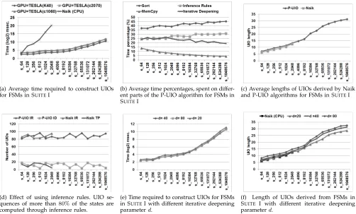
We present the mean timing results in Figure 13a. As expected, when the size of the FSM grows, the time required to construct UIOs increases. We observe that Naik’s approach took less than three seconds on average to generate UIOs for FSMs with 512 states. For FSMs with1024states the time rises to68.45seconds, for FSMs with 2048 states the average time to construct UIOs is
1231 seconds. Therefore we did not process FSMs with more than 2048 states. These results suggest that the P-UIO algorithm can increase the scalability of Naik’s algorithm by a factor4 of 512.
The results show that when the NVIDIA TESLA K40 card was used, UIOs for very large FSMs (FSMs with 1 million states) could be constructed in less than two sec-onds (1626 msec on average). With the TESLA c2070 card the average time required increased to 3170 msec. and with the TESLA c1060 card the average time increased to 3658 msec. In Table 2 we provide the reduction in timings. The results for SUITEI indicate that P-UIO can
be11000times faster then the existing UIO construction
algorithm on average.
In Figure 13b we present the distribution of time spent by the P-UIO algorithm where Sort, Inference Rules, MemCpy, and Iterative Deepening stand for the average time spent for sorting, average time spent for finding new UIOs using inference rules, average time spent for memory transactions between the CPU and the GPU and the average time spent for IDP respectively.
The results suggest that most of the time required to construct UIO sequences was spent on sorting (averages vary between 37.6% and 45.01%) and we also observe that the use of inference rules took25%−30%of the time on average, which (compared to time spent on sorting) was not expected. Therefore we investigated the effect of using inference rules by counting the number of UIOs found using inference rules and the number of UIOs found during exploration. Figure 13d summarises the results.
The results suggest that on average at least 80% of the UIOs were found using inference rules. These results justify the time spent on inference rules. In addition, the average percentage of time used for back-tracking (Memcpy) and iterative deepening reduces as the size of the FSM increase. This implies that as we increase the number of states, the utilisation of the GPU increases.
Figure 13c gives the results regarding UIO length. Note that the length of the UIOs returned by the P-UIO
4. The P-UIO algorithm could process FSMs with220 states and
Naik’s algorithm could process FSMs with211 states hence we have
(a) Average time required to construct UIOs for FSMs in SUITEI
(b) Average time percentages, spent on differ-ent parts of the P-UIO algorithm for FSMs in SUITEI
(c) Average lengths of UIOs derived by Naik
and P-UIO algorithms for FSMs in SUITEI
(d) Effect of using inference rules. UIO
se-quences of more than80%of the states are
computed through inference rules.
(e) Time required to construct UIOs for FSMs in SUITEI with different iterative deepening
parameterd.
(f) Length of UIOs derived from FSMs in
SUITE I with different iterative deepening
[image:14.612.56.558.61.364.2]parameterd.
Figure 13: Results of experiments on test SUITEI.
s64 s128 s256 s512 s1024 s2048 Avg.
T(Naik)/T(P-UIOT ESLA(K40)) 1.56 33.70 79.56 316.99 6001.64 104091.79 18420.88
T(Naik)/T(P-UIOT ESLA(K20))) 0.78 16.20 41.44 166.84 2956.47 49567.52 8791.54
T(Naik)/T(P-UIOC1060)) 0.76 15.60 34.00 126.79 2655.59 45454.93 8047.95
Avg. 1.04 21.83 51.67 203.54 3871.24 66371.41 11753.45
Table 2: The ratio of computation times.
algorithm does not depend on the underlying card and so we present the results obtained from the TESLA K40 GPU card. The results suggest that compared to the P-UIO algorithm, Naik’s approach can find shorter P-UIOs (13% shorter on average). This result may be caused by the iterative deepening process. As the P-UIO algorithm iteratively deepens an IO-vector until it reaches depthd, it need not find the shortest UIOs. To investigate this we performed a set of experiments and repeated the tests on the P-UIO algorithm with different dvalues.
The results are presented in Figure 13e and Figure 13f. These results suggest that as we decrease the depth parameter (to d = 20), the time required to construct UIOs increases. This is because as we decrease d, the performance of the GPU reduces due to the frequent memory copy operations. However, the length of the UIO sequences reduces: whend= 20, the average differ-ence between the length of UIO sequdiffer-ences constructed by the Naik and the P-UIO algorithms reduces to6%. On the other hand, as we increase the iterative deepening parameter d to d = 80 again the time required to construct UIOs increases. This may be due to the fact
that as we increase d, we also increase the amount of data that is sorted after IDP. Moreover, when we use
d= 80the length of the UIOs increase: Naik’s algorithm generates UIOs that are 38% shorter compared to the P-UIO algorithm on the average.
During the experiments we observed that some FSMs did not have UIOs for every state. We observe that as the number of states increase the chance of generating FSM reduces. In order to generate100FSMs that have a UIO for each state we generated232FSMs whenn= 64,
422 FSMs when n= 128, 628 FSMs when n= 256,839
FSMs when n = 512, 1097 FSMs when n = 1024, 1265
FSMs when n= 2048,1322 FSMs when n= 4096, 1493
FSMs whenn= 8192,1755FSMs whenn= 16384,1959
FSMs whenn= 32768,2103FSMs whenn= 65536,2395
FSMs when n = 131072, 2595 FSMs when n = 262144,
2797 FSMs when n = 524288 and 2903 FSMs when
n = 1048576. Recall that if UIOs are not found for all
states then one can instead use a characterising set that contains at mostn−1sequences of length at mostn−1
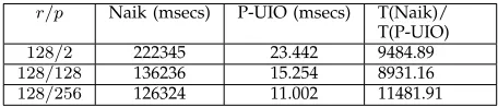
[image:14.612.113.497.391.444.2]r/p Naik (msecs) P-UIO (msecs) T(Naik)/ T(P-UIO)
128/2 222345 23.442 9484.89
128/128 136236 15.254 8931.16
[image:15.612.60.288.54.103.2]128/256 126324 11.002 11481.91
Table 3: Average time to construct UIOs for FSMs in SUITEII and average increment in timings.
r/p Naik P-UIO L(Naik)/
L(P-UIO)
128/2 10.82 17.27 0.62
128/128 10.27 11.35 0.90
128/256 11.45 11.27 1.01
Table 4:Average length of UIOs for FSMs in SUITEII.aaaaa
5.2.2 Results of experiments for FSMs inSUITEII
The time required to construct UIOs for FSMs in SUITE
II is given in Table 3. Throughout these experiments we set d = 40. As expected, as the number of outputs increases, the time required to construct UIOs decreases. We observe that one particular reason for this is that as the number of outputs increases the length of the UIOs derived from FSMs tends to reduce (Table 4). This is to be expected: as the number of outputs increases, the algorithms (Naik, P-UIO) have more opportunities to split states, hence the length of the UIOs reduce. However, we see that the performance of the P-UIO algorithm is far better than that of Naik’s algorithm (9900
times faster on average).
5.2.3 Results of experiments for FSMs inSUITEIII
The results are presented in Table 5 where we setd= 40. The time required to construct UIOs with Naik’s al-gorithm and the P-UIO alal-gorithm (with the Tesla K40 card) are similar for FSMs dk27, bbtas, dk17, and dk15. Moreover, for these FSMs the P-UIO algorithm is slower when Tesla C2070 and C1060 were used. However, as the FSMs get larger the time required to construct UIO with Naik’s approach increases faster than that required by the P-UIO algorithm. As before, we also observe that the UIOs found are shorter when Naik’s approach is used.
5.3 Threats to validity
This section briefly reviews threats to validity and how these were reduced. We consider threats to internal validity, construct validity, and external validity.
Threats to internal validity concern factors that might introduce bias. The main source of such threats is the tools used to run the experiments. The FSM generation tool has been used in a number of projects and was tested. The implementations of the two algorithms were carefully checked and also tested with a range of FSMs. To further reduce this threat, we also used an existing tool that checks if an input sequence is a UIO for the FSM. This tool was used to check all of the UIOs generated by the P-UIO algorithm and Naik’s approach.
Another threat to internal validity concerns the ran-dom process employed while selecting input sequences: the order of selection may effect the performance of the algorithm. To investigate this factor, we repeated each experiment on Test SUITE III 100 times. The results are
provided in Table 6. We observe that, except for the specification named planet, the variance of timing and length of UIOs are low, that is to say for this set of FSMs the random input selection process has limited effect.
Threats to construct validity reflect the potential for the measurements made to not reflect properties that are of interest in practice. The main focus of our study was the time taken to generate UIOs and, as a result, the scalability of the algorithm. We want FSM-based test generation techniques that scale to large FSMs and so scalability is important. Note that FSMs are likely to be particularly large when one cannot abstract out all of the data of a model, since we then obtain a separate state for each logical state of the model combined with each possible combination of values for the model’s variables. However, to reduce the scope for threats to construct validity we also recorded the mean UIO length.
Threats to external validity concern our ability to generalise from the experiments. There is always such a threat to validity since we do not know the space of relevant FSMs and certainly have no good way of sampling from this. We reduced this threat by using a combination of randomly generated FSMs and FSMs from industry that are in a benchmark. We also varied the number of outputs and states.
5.4 Discussion
Recall that in Section 3 we observed that the P-UIO algo-rithm is an exponential algoalgo-rithm; this cannot be avoided since determining the existence of UIOs is PSPACE-hard. As the length of the UIO sequences generated from the FSMs in SUITE I and SUITE II are not longer than the logarithm of the number of states, it appears that we have not found such long executions. However, it has been reported [12] that this is usual: the length UIO sequences are often no longer than the logarithm of the number of states of the FSM. Another important point is the need to select parameterd. The experiments revealed that when we select a value for d that is too large, the algorithm gets slower as the size of data to be sorted increases. However, ifdis too small then this may decrease the GPU occupancy and increasing the traffic between the CPU memory and the GPU memory. Therefore, the parameterdshould be selected carefully.