Topics in Gravitational-Wave Science: Macroscopic Quantum Mechanics and Black Hole Physics

(1)

Topics in Gravitational-Wave Science: Macroscopic

Quantum Mechanics and Black Hole Physics

Thesis by

Huan Yang

In Partial Fulfillment of the Requirements for the Degree of

Doctor of Philosophy

California Institute of Technology Pasadena, California

2013

(2)

c

2013

(3)

Dedicated to my parents

(4)

Acknowledgments

There is a Chinese saying that goes, “it takes ten years to sharpen a sword.” It took me the continuous effort of many years to become an qualified “sword” (with a Ph.D.), ready for cutting through the fog of unknowns at the frontier of physics. Along my way, studying physics during these years, I have received enormous encouragement and assistance from my family, my friends and my colleagues. I am grateful for the help of all of them, and I shall acknowledge them in chronological order.

First I would like to thank my parents Fuxi Yin and Ganqin Yang. They taught me the really important things in life and they showed me how to build my character with integrity, honesty and sheer tenacity. There were times when I was confused and uncertain about my future, but they always told me to follow my heart and they always supported my decisions. My parents greatly helped me to define who I am.

I am also thankful to Kip Thorne and Nai-Chang Yeh. I worked with Kip since my sophomore year. He brought me into the field of general relativity, which has become one of my main research interests. He influenced me not only through his scientific wisdom, but also his way of interacting with people and his positive energy. Nai-Chang was my senior thesis advisor. During my time working in her lab, I was truly impressed by her passion and attitude toward doing research. As a female professor, she is also very generous to her students. I would like to thank for all her help in my past studies.

I want to give special thanks to my Ph.D thesis advisor Yanbei Chen. As an advisor and as a physicist, he is my favorite type: very considerate to students, always curious about problems in physics and full of ideas. I enjoyed spontaneous discussions with him about many branches of physics, and I learned a lot from him about ways of looking at and solving physics problems. I am also grateful for his encouragement and painstaking effort to teach me how to write scientific articles and give clear presentations .

(5)

and many of them have turned into chapters of this thesis.

I would like to acknowledge Stefan Danilishin, Thomas Corbitt, Kentaro Somiya, Yiqiu Ma, Farid Khalili and Sergey Vyatchanin and all the other members of the Macroscopic Quantum Mechanics (MQM) discussion group. I also want to thank other colleagues outside Caltech: Howard Wiseman, Scott Hughes, Emanuele Berti, Sam Dolan, Marc Casals, Yi Pan, Steven Detweiler, Steve Carlip, Da-Shin Lee, Bei-lok Hu, Ting Yu, Walter Strunz, Matthew Evans and Ian Vega. I enjoyed and benefitted from stimulating discussions with all of them.

I want to thank the two other members of my thesis committee who have not been mentioned before: Christopher Hirata and Christian Ott, for giving me very valuable advice and comments on my thesis research as well as presentation skills.

In working on chapters of this thesis, I was supported by the following public funding: NSF Grants PHY-1068881 and PHY-1005655, CAREER Grants PHY-0956189 and PHY-1055103, NASA Grant No.NNX09AF97G, the Sherman Fairchild Foundation and the Brinson Foundation. I am also grateful for the donation from Dr. and Mrs. David and Barbara Groce, whose gift enabled me to finish my Ph.D. degree in physics.

(6)

Abstract

The theories of relativity and quantum mechanics, the two most important physics discoveries of the 20th century, not only revolutionized our understanding of the nature of space-time and the way matter exists and interacts, but also became the building blocks of what we currently know as modern physics. My thesis studies both subjects in great depths — this intersection takes place in gravitational-wave physics.

Gravitational waves are “ripples of space-time”, long predicted by general relativity. Although in-direct evidence of gravitational waves has been discovered from observations of binary pulsars, in-direct detection of these waves is still actively being pursued. An international array of laser interferometer gravitational-wave detectors has been constructed in the past decade, and a first generation of these detectors has taken several years of data without a discovery. At this moment, these detectors are being upgraded into second-generation configurations, which will have ten times better sensitivity. Kilogram-scale test masses of these detectors, highly isolated from the environment, are probed con-tinuously by photons. The sensitivity of such a quantum measurement can often be limited by the Heisenberg Uncertainty Principle, and during such a measurement, the test masses can be viewed as evolving through a sequence of nearly pure quantum states.

The first part of this thesis (Chapter 2) concerns how to minimize the adverse effect of thermal fluctuations on the sensitivity of advanced gravitational detectors, thereby making them closer to being quantum-limited. My colleagues and I present a detailed analysis of coating thermal noise in advanced gravitational-wave detectors, which is the dominant noise source of Advanced LIGO in the middle of the detection frequency band. We identified the two elastic loss angles, clarified the different components of the coating Brownian noise, and obtained their cross spectral densities.

(7)

measurement processes. Chapter 4 establishes a mathematical formalism that describes the evolution of a quantum system (the plant), which is coupled to a non-Markovian bath (i.e., one with a memory) while at the same time being under continuous quantum measurement (by the probe field). This aims at providing a general framework for analyzing a large class of non-Markovian measurement processes. Chapter 5 develops a way of characterizing the non-Markovianity of a bath (i.e.,whether and to what extent the bath remembers information about the plant) by perturbing the plant and watching for changes in the its subsequent evolution. Chapter 6 re-analyzes a recent measurement of a mechanical oscillator’s zero-point fluctuations, revealing nontrivial correlation between the measurement device’s sensing noise and the quantum rack-action noise.

Chapter 7 describes a model in which gravity is classical and matter motions are quantized, elaborating how the quantum motions of matter are affected by the fact that gravity is classical. It offers an experimentally plausible way to test this model (hence the nature of gravity) by measuring the center-of-mass motion of a macroscopic object.

The most promising gravitational waves for direct detection are those emitted from highly en-ergetic astrophysical processes, sometimes involving black holes — a type of object predicted by general relativity whose properties depend highly on the strong-field regime of the theory. Although black holes have been inferred to exist at centers of galaxies and in certain so-called X-ray binary objects, detecting gravitational waves emitted by systems containing black holes will offer a much more direct way of observing black holes, providing unprecedented details of space-time geometry in the black-holes’ strong-field region.

The third part of this thesis (Chapters 8 – 11) studies black-hole physics in connection with gravitational-wave detection.

(8)

Topics in gravitational wave detectors

36

2 Brownian thermal noise in multilayer coated mirrors 37 2.1 Introduction . . . 37

2.2 Components of the coating thermal noise . . . 40

2.2.1 Complex reflectivity . . . 40

2.2.2 Thermal Phase and Amplitude Noise . . . 41

2.2.3 Fluctuationsδφj andδrp . . . 43

2.2.4 Mode selection for phase noise . . . 46

2.2.5 Conversion of amplitude noise into displacement . . . 46

2.3 Thermal noise assuming no light penetration into the coating . . . 47

(10)

2.3.2 Mechanical energy dissipations in elastic media . . . 48

2.3.3 Thermal noise of a mirror coated with one thin layer . . . 50

2.3.4 Discussions on the correlation structure of thermal noise . . . 52

2.4 Cross spectra of thermal noise components . . . 53

2.4.1 Coating-thickness fluctuations . . . 53

2.4.2 Fluctuations of Coating-Substrate Interface and their correlations with coating thickness . . . 55

2.4.3 The anatomy of coating thermal noise . . . 57

2.4.4 Full formula for thermal noise . . . 60

2.5 Effect of light penetration into the coating . . . 61

2.5.1 Optics of multi-layer coatings . . . 62

2.5.2 Levels of light penetration in Advanced LIGO ETM Coatings . . . 63

2.5.3 Thermal noise contributions from different layers . . . 65

2.6 Dependence of thermal noise on material parameters . . . 66

2.6.1 Dependence on ratios between loss angles . . . 66

2.6.2 Dependence on Young’s moduli and Poisson’s ratios . . . 69

2.6.3 Dependence on photoelastic coefficients . . . 70

2.6.4 Optimization of coating structure . . . 70

2.7 Measurements of loss angles . . . 72

2.7.1 Bending modes of a thin rectangular plate . . . 73

2.7.2 Torsional modes of a coated hollow cylinder . . . 74

2.8 Conclusions . . . 75

2.A Fluctuations of the complex reflectivity due to refractive index fluctuations . . . 79

2.A.1 The photoelastic effect . . . 79

2.A.2 Fluctuations in an infinitesimally thin layer . . . 80

2.A.3 The entire coating stack . . . 81

2.A.4 Unimportance of transverse fluctuations . . . 83

2.B Elastic deformations In the coating . . . 83

2.C Definition of loss angle . . . 86

2.D Advanced LIGO style coating . . . 88

II

Topics in macroscopic quantum mechanics

91

3 Open quantum dynamics of single-photon optomechanical devices 92 3.1 Introduction . . . 92

(11)

3.2.1 The Hamiltonian . . . 95

3.2.2 Structure of the Hilbert space . . . 96

3.2.3 Initial, final States and photodetection . . . 98

3.2.4 Evolution of the photon-mirror quantum state . . . 99

3.2.4.1 Free evolution . . . 99

3.2.4.2 Junction condition . . . 101

3.2.4.3 Coupled evolution . . . 101

3.2.4.4 Full evolution . . . 102

3.3 Single-photon interferometer: Visibility . . . 103

3.3.1 The configuration . . . 103

3.3.2 The role of the beamsplitter and a decomposition of field degrees of freedom 104 3.3.3 Interactions between light and cavities . . . 105

3.3.4 The final state . . . 107

3.3.5 Examples . . . 108

3.4 Conditional quantum-state preparation . . . 111

3.4.1 The configuration . . . 111

3.4.2 Preparation of a single displaced-Fock state . . . 112

3.4.3 Preparation of an arbitrary state . . . 116

3.5 Practical considerations . . . 118

3.6 Conclusions . . . 119

4 Towards understanding non-Markovian quantum measurement 122 4.1 Introduction . . . 122

4.2 Quantum-classical interface: the measurement device . . . 123

4.3 Markovian measurement of a cavity mode . . . 125

4.4 Non-Markovian quantum measurement: the first scenario . . . 127

4.4.1 Cavity QED: atom-cavity interaction . . . 127

4.4.2 Optomechanical device . . . 130

4.4.3 Generalization to bath with many degrees of freedom . . . 131

4.5 Non-Markovian quantum measurement: The second scenario . . . 134

4.5.1 linear continuous measurement . . . 135

4.5.2 Phonon number measurement . . . 140

4.5.3 Nonlinear measurement with initially entangled detector state . . . 142

4.6 Non-Markovian quantum measurement: General case . . . 143

4.7 Conclusion . . . 143

(12)

4.B SME for measurement of cavity mode . . . 146

4.C Operator ˆO in the linear coupling case . . . 147

4.D Operator ˆO for optomechanical interaction . . . 149

4.E Operator ˆOk in the linear coupling case . . . 150

4.F Perturbative solution of ˆOk . . . 151

5 Revealing non-Markovianity of open quantum systems via local operations 155 5.1 Introduction . . . 155

5.2 Plant – bath dynamics . . . 157

6 Quantum back-action in measurements of zero-point mechanical oscillations 164 6.1 Introduction . . . 164

6.2 A two-beam experiment that measures zero-point mechanical oscillation . . . 167

6.2.1 Experimental setup and results . . . 168

6.2.2 Interpretation in terms of quantum measurement . . . 169

6.2.2.1 The mechanical oscillator near ground state . . . 169

6.2.2.2 The quantum-measurement process . . . 170

6.2.2.3 Asymmetry between spectra . . . 171

6.2.3 Detailed theoretical analysis . . . 172

6.2.4 Connection with the scattering picture . . . 174

6.3 General linear measurements of the zero-point fluctuation . . . 177

6.3.1 The nature of zero-point mechanical fluctuation . . . 177

6.3.2 Measuring the zero-point fluctuation . . . 179

6.3.3 Measuring an external classical force in presence of zero-point fluctuation . . 181

6.A Symmetrized cross spectral density . . . 184

6.B Commutation relation between ˆz and ˆF . . . 184

7 Macroscopic quantum mechanics in a classical spacetime 188 7.1 Introduction . . . 188

7.2 SN theory for macroscopic objects . . . 190

7.3 Discussion and conclusion . . . 196

7.A Supplementary material for macroscopic quantum mechanics in a classical spacetime 197 7.A.1 A. Incompatibility between the many-world interpretation of quantum me-chanics and classical gravity . . . 197

(13)

7.A.3 C. Effective Heisenberg equations of motion and coupling with optical field . 199

7.A.4 D. SN Equation for two macroscopic objects . . . 201

III

Topics in black hole perturbation theory

205

8 First-order perturbative hamiltonian equations of motion for a point particle orbiting a Schwarzschild black hole 206 8.1 Introduction . . . 207

8.2 Review of Moncrief’s Hamiltonian approach . . . 210

8.2.1 First-order perturbation of a static space-time in 3+1 form . . . 210

8.2.2 Degrees of freedom . . . 211

8.2.3 Schwarzschild perturbations . . . 213

8.2.4 Odd parity (l≥2) . . . 214

8.2.5 Even parity (l≥2) . . . 216

8.2.6 Monopole and dipole perturbations . . . 218

8.3 3+1 approach with point mass source . . . 218

8.3.1 3+1 Formulation . . . 218

8.3.2 Odd parity (l≥2) . . . 220

8.3.3 Even parity (l≥2) . . . 222

8.4 Regularization of test particle equation of motion . . . 226

8.4.1 General Discussion . . . 226

8.4.2 Odd parity . . . 228

8.4.2.1 An algebraic gauge . . . 228

8.4.2.2 Fixing Lorenz gauge . . . 230

8.4.3 Even parity . . . 231

8.5 Conclusions and discussions . . . 234

8.A Various tensor spherical harmonics . . . 236

8.B Conversion of fields for even parity perturbations . . . 236

9 Quasinormal-mode spectrum of Kerr black holes and its geometric interpretation240 9.1 Introduction . . . 241

9.1.1 Overview of quasinormal modes and their geometric interpretation . . . 241

9.1.2 Methods and results of this article . . . 243

9.1.3 Organization of the paper . . . 245

(14)

9.2.1 The Teukolsky equations . . . 246

9.2.2 The angular eigenvalue problem . . . 247

9.2.2.1 Real part ofAlm for a real-valuedω . . . 248

9.2.2.2 ComplexAlm for a complexω . . . 251

9.2.3 The radial eigenvalue problem . . . 252

9.2.3.1 ComputingωR . . . 252

9.2.3.2 ComputingωI . . . 255

9.2.4 Accuracy of the WKB approximation . . . 256

9.3 Geometric optics in the Kerr spacetime . . . 260

9.3.1 Geometric optics: general theory . . . 260

9.3.2 Null geodesics in the Kerr spacetime . . . 262

9.3.3 Correspondence with quasinormal modes . . . 263

9.3.3.1 Leading order: conserved quantities of rays and the real parts of quasinormal-mode parameters . . . 263

9.3.3.2 Next-to-leading order: radial amplitude corrections and the imagi-nary part of the frequency . . . 266

9.3.3.3 Next-to-leading order: angular amplitude corrections and the imag-inary part of Carter’s constant . . . 271

9.4 Features of the spectra of Kerr black holes . . . 273

9.4.1 Spherical photon orbits and extremal Kerr black holes . . . 273

9.4.2 A mode’s orbital and precessional frequencies . . . 276

9.4.3 Degenerate quasinormal modes and closed spherical photon orbits . . . 278

9.4.3.1 Slowly spinning black holes . . . 280

9.4.3.2 Generic black holes . . . 281

9.5 Conclusions and discussion . . . 281

9.A The Taylor expanded Bohr-Sommerfeld condition . . . 283

10 Branching of quasinormal modes for nearly extremal Kerr black holes 287 10.1 Introduction . . . 287

10.2 Matched expansions . . . 289

10.3 WKB analysis . . . 291

10.4 Phase boundary . . . 292

10.5 Bifurcation . . . 293

10.5.1 Numerical investigation . . . 293

10.5.2 Bound state formulation of the radial Teukolsky equation . . . 295

(15)

10.A Numerical methods . . . 301

10.B Criteria for phase boundaries for electromagnetic and gravitational modes . . . 301

11 Scalar wave propagation in Kerr spacetime 306 11.1 Introduction . . . 306

11.2 Spectral decomposition . . . 307

11.3 QNMs in the eikonal limit . . . 310

11.3.1 The radial wavefunction . . . 311

11.3.2 The angular wavefunction . . . 312

11.4 Matched expansions . . . 314

11.4.1 Wavefunction near the peak of the scattering potential . . . 315

11.4.2 WKB wavefunctions away from the peak of the scattering potential . . . 316

11.4.3 Matching solutions . . . 318

11.5 The Green fucntion . . . 320

11.5.1 Summation over of all QNM contributions and the singular structure . . . 320

11.5.2 The Green function . . . 322

(16)

Chapter 1

Introduction

This thesis is an assembly of ten research papers that span across several disciplines of physics, which are all related to the on-going effort of gravitational-wave detection. According to the different aspects of gravitational-wave science they involve, the following ten chapters of this thesis can be naturally divided into three parts. In Part I (Chapter 2), we study the physics of advanced gravitational-wave detectors, in particular how thermal fluctuations affect the detectors’ sensitivity. In Part II (Chapters 3 – 7), motivated by the fact that gravitational-wave detectors are continuously monitoring kilogram-scale test masses near the quantum limit, we study Macroscopic Quantum Mechanics. In Part III (Chapters 8 – 11), we study physics of gravitational-wave sources, in particular black-hole perturbation theory. Correspondingly, this introductory chapter has also been divided into three sections. In each section, we shall first provide background for the corresponding part of the thesis, and then briefly discuss the motivation and summarize the main results of each chapter in that part.

1.1

Physics of advanced gravitational wave detectors

1.1.1

An overview of laser interferometer gravitational-wave detectors

(17)

In the past five years, an international array of first-generation long-baseline laser-interferometer GW detectors have operated at their design sensitivities. This array included: the LIGO detectors (US, two 4 km detectors H1 and L1, one 2 km detector H2) [2], the VIRGO detector (France and Italy, 3 km) [3], the GEO 600 detector (UK and Germany, 600 m) [4] and the TAMA detector (Japan, 300 m) [5]. Up till now, with most of the first-generation data analysis finished, no direct detection of GW has been made, and this is consistent with astrophysical estimates. In order to achieve first detection, and subsequently develop a fruitful observational program of GW astronomy, the GW community must keep upgrading their detectors for better sensitivity. At this moment, while second-generation detectors (for example the Advanced LIGO detectors in the US) are in construction, experimental techniques aimed for third-generation detectors are being researched and prototyped. These prototype experiments include: the 300-m CLIO cryogenic detector (Kamioka, Japan) [6], the AEI 10-m prototype (under construction in Hannover, Germany) [7], the Glasgow 10-m prototype (Glasgow, UK) [8], the 80-m high-power facility (Gingin, Australia) [9], and table-top experiments with small test masses (MIT/ANU/NAOJ) [10].

The typical configuration of a long-baseline laser interferometer GW detector is a Michelson interferometer with km-scale arms and kg-scale suspended test masses serving as mirrors. The suspension frequencies are usually around 1 Hz, therefore allowing the isolation of ground motion at frequencies∼10 Hz and above — at these frequencies, the test masses act as free masses. Laser light is incident from, and mostly returns to the “bright port” of the Michelson interferometer — if the mirrors remain at their equilibrium positions — and in this case only a small amount of light is allowed to emerge from the “dark port” of the interferometer. As arm lengths change differentially (e.g., due to incoming GWs), additional signal light emerges from the dark port. At the photodetector, the signal light beats with the static output light from the dark port to give a linear signal proportional to the amplitude of the gravitational wave. Optical cavities are often used in the arms (therefore there are two mirrors in each arm) in order to increase light power in the arms and amplify the signal light. The interferometer’s performance is further amplified when “recycling mirrors” are further placed at the bright and dark ports.

As we consider GWs with frequencies below the free spectral range of the arm cavity, i.e.,c/(2L) (withLthe arm length, 10s of kHz) and above the resonant frequency of the test masses’ translational motion, a gravitational wave with amplitude h can be viewed as causing relative displacements

∼ Lh/2 between the mirrors (with a geometrical factor that depends on its polarization), while

causing no effect on the propagation of light. We can therefore regard GW detectors as displacement measuring devices; their sensitivity for measuring the displacement is limited byforce noiseswhich disturb the motion of test masses, andreadout noiseswhich add random output fluctuations to the displacement signal. These noises may have both classical and quantum origins (see Fig. 1.1).

(18)

Figure 1.1: (Color online.) Square root of strain noise spectrum for several of Advanced LIGO’s major noise sources. In its detection band 10 Hz – several kHz, Advanced LIGO’s sensitivity is mainly constrained by quantum noise and coating Brownian noise (red curve).

noise spectral density). This figure shows several major types of noise that are of classical origin [11]:

• Suspension thermal noise (blue curve in Fig. 1.1), which arises from thermal fluctuations in the wires that are used to suspend the test masses.

• Gravity gradient noise (dark green curve in Fig. 1.1), which arises from differential fluctua-tions of the Newtonian gravitational field at the locafluctua-tions of the test masses. The dominant component of this noise arises due to surface seismic waves [12].

• Excess gas noise(light green curve in Fig. 1.1), which is mainly produced by gas molecules in the beam tube. The high frequency component of this noise arises from molecules randomly moving through the laser beam, causing phase noise, while at low frequencies the random impacts of molecules on the mirror surfaces dominate [13].

• Seismic noise (brown curve in Fig. 1.1), which is the mirror position fluctuation induced by ground vibrations. It is the main noise source below 10 Hz.

(19)

of the coating and random variations in the coating materials’ refractive index. The geometric deformation affects the position of the mirror surface, causing thermoelastic noise, while the refractive index change affects the phase probed by the light beam, which partially penetrates into the coating layers, causing thermorefractive noise. Evans et al. proved that by careful design of coating structure these two pieces of noise can almost cancel each other in Advanced LIGO mirrors[15].

• Brownian noise (red curve in Fig. 1.1), which includes coating Brownian noise and substrate Brownian noise. At constant temperature T, each elastic eigenmode of the mirror possesses

kBTenergy according to equal partition theorem. Because of the mechanical losses, the thermal spectrum of these modes all have a tail to the low frequency end, and the sum of all these contributions gives the Brownian noise. Because coatings (quality factor∼103_{) are much more} lossy than the substrate (quality factor ∼107₋₁₀8_{), coating Brownian noise is much higher} than substrate Brownian noise, and turns out to be higher than all other classical noises in the advanced LIGO detection band. This is the main motivation for us to carefully analyze coating Brownian noise in Chapter 2.

In Fig. 1.1, quantum noise is shown in purple curve. This includes quantum radiation pressure noise, photon shot noise and sensing noise due to optical loss and inefficient photo-detection. The sensing noise due to optical or photo-detection loss is an important component of the quantum noise budget, but it can be improved by using better optical systems. The shot noise and radiation pressure noise together is often subject to a sensitivity bound for general quantum measurement, as will be shown below (and in the Section 1.2 from a different perspective). Let us approximate LIGO mirrors as free masses and, for simplicity, assume there are no arm cavities. The displacement-referred noise spectrum due to radiation-pressure fluctuation for a free massmis

Srp_x(Ω) = I0ω0~

m2_Ω4_c2, (1.1)

where ω0 is the angular frequency of the laser beam and I0 is the optical power. The stronger the power of the laser, the higher the rate of random photons that will impinge on the mirror, hence the higher the radiation-pressure noise. On the other hand, the displacement-referred spectrum of shot noise is

S_xsh= ~c 2

I0ω0

(1.2)

which is inversely-proportional to the number of sensing photons — increasing the rate of sensing photons will improve the our accuracy of position measurement.

(20)

asStandard Quantum Limit(SQL) as first realized by Braginsky in the 1960s [17, 18]:

Sx=Sxrp+Sxsh= I0ω0~

m2_Ω4_c2 +

~c2

I0ω0

≥SxSQL(Ω)≡

2~

mΩ2. (1.3)

Here m =M/4 is the reduced mass of the four test masses (each with a mass ofM). As we will show later in Sec. 1.2, once these GW detectors enter this quantum regime, in addition to detecting gravitational waves with higher sensitivity, one can also use these interferometers to probe quantum behaviors of macroscopic test masses. In this case, SQL serves as a benchmark for a successful macroscopic quantum mechanics (MQM) experiment.

1.1.2

Brownian thermal noise of mirrors with multilayer coatings

(Chap-ter 2)

Chapter 2 is a research paper published as:

• T. Hong, H. Yang, E.K. Gustafson, R.X. Adhikari and Y. Chen, Brownian thermal noise in multilayer coated mirrors, Physical Review D87, 082001 (2013).

1.1.2.1 Motivation and significance

(21)

1.1.2.2 Summary of main results

We start Chapter 2 by expressing the amplitude and phase of the reflected light in terms fluctuations in all aspects of the coating structure, thereby identifying all components of coating thermal noise. For example, we show that coating noise arise not only from layer thickness fluctuations (as one might naively think at first sight), but also from fluctuations of the interface between the coating and substrate, which can also be driven by internal fluctuating stresses of the coating. After applying the fluctuation-dissipation theorem, we find that thickness fluctuations of different coating layers are incoherent with each other, although they may correlate with fluctuations of the coating-substrate interface (depending on the loss angles, which will be discussed later). This is because the fluctuating stress in any coating layer does not affect thicknesses of the other layers, yet it may influence the bending of coating-substrate interface. Based on the formulas we obtained for cross spectral densities, roughly 70% of Advanced LIGO’s coating Brownian noise is due to coating-substrate interface fluctuations, because Young’s modulus of the more lossy type of coating material (Ta2O5) was assumed to be much higher than the Young’s modulus of the substrate. This piece of noise turns out to be inversely proportional to the Young’s modulus of the substrate material, which means it can be reduced by using stiffer substrate materials.

Previously [43], the vertical and horizontal loss anglesφ⊥, φkof an isotropic material are defined

such that given a periodic driving force, the energy dissipated per radian is

Wdiss =φ⊥U⊥+φkUk, Utot=U⊥+Uk (1.4)

where the total elastic energy Utot is separated into vertical component U⊥ (perpendicular to the

surface) and horizontal component Uk (parallel to the surface). In Chapter 2, we show that for

materials with nonzero poisson ratios, U⊥ and Uk could be negative for certain ways of applying

external forces. This means neither U⊥ norUk is a reasonable candidate for energy. We instead

propose to use shear and bulk loss anglesφΣ, φΘ, associated with the bulk and shear elastic energy such that

Wdiss=φΣUΣ+φΘUΘ, Utot=UΣ+UΘ. (1.5)

(22)

proposed experiment with previous measurements, bulk and shear loss angles can be determined separately.

In Chapter 2 we also point out a new contribution to coating Brownian noise that had not been discussed before. As briefly explained earlier, this noise is due to refractive-index fluctuations induced by strain fluctuations, via the photoelastic effect. The photoelastic noise not only imposes a fluctuating phase shift to light propagating within the coating — the inhomogeneity caused by this noise also back-scatters some of the propagating light. All the backscattered light add up together to a new piece of phase noise, which we refer as “backscattered noise”. There is one subtlety we encountered when computing this noise — mathematically the self correlation of Brownian strain fluctuations is a δ function in position space, and so is the resulting refractive-index fluctuation. Thisδfunction apparently causes a divergence problem during the calculation of the backscattered noise. Fortunately, since the average of fluctuations over any small volume is finite, the total noise is in fact regular. After a careful treatment, we successfully obtained a regular expression for the back-scattered noise. For advanced LIGO coatings, the back-back-scattered noise is less than 5% of the total coating Brownian noise, because light only penetrates into the first few coating layers, and because the back-scattering is relatively weak in the first place. However, for other optics experiments using mirrors with far fewer coating layers, this could be a more important part of total coating Brownian noise.

1.1.2.3 My specific contributions

I derived the formulas for cross spectral density between strain fluctuations at different locations, and I also did the calculation for back-scattered noise. I was in charge of revising the manuscript and answering questions from the referees during the peer-review process and production stages.

1.2

Macroscopic Quantum Mechanics (MQM)

1.2.1

Background

(23)

successfully preparing one degree of freedom of a macroscopic object into the quantum ground state [19], as well as generating squeezed light though its interaction with a macroscopic oscillator [20]. There are several excellent review articles on this subject: one of them is written by Chen [21], which emphasizes quantum measurement and testing quantum mechanics; the other one is written by Aspelmeyer, Kippenberg and Marquart [22], which discusses cavity optomechanics from an ex-perimental point view. In this section we will only discuss a few basics that are relevant for Part II of this thesis.

1.2.1.1 The input-output formalism of linear quantum measurement theory

Let us illustrate the input-output formalism of linear quantum measurement theory using a simple example. Suppose a laser beam with intensityI0and frequencyω0is targeting on a test object with massm and mechanical frequency ωm. With phase reference (the plane where the phase is set to zero) chosen at the equilibrium position of the test object, the input electrical field can be written as

ˆ

Ein(t) =hp2I0/~ω0+ ˆa1(t)

i

cosω0t+ ˆa2(t) sinω0t (1.6)

with ˆa1,ˆa2being the amplitude and phase quadratures of the fluctuation, their cross spectral density given by:

Sa₁(Ω) =Sa₂(Ω) = 1, Sa₁a2(Ω) = 0. (1.7)

The reflected electric field ˆEout(t) is just

ˆ

Eout(t) = ˆEin(t−2ˆx/c), (1.8)

where 2ˆx/cis the extra delay time. Similar to the input field, the output field can also be decomposed as:

ˆ

Eout(t) =hp2I0/~ω0+ ˆb1(t)

i

cosω0t+ ˆb2(t) sinω0t . (1.9)

According Eq. (1.8), the output quadrature fields ˆb1,ˆb2and input quadrature fields ˆa1,aˆ2are related to each other by

ˆ

b1(t) = ˆa1(t) (1.10)

ˆ

b2(t) = ˆa2(t) + 2

r

2I0ω0

~c2

ˆ

x. (1.11)

(24)

the other hand, the Heisenberg equations of motion of the test object are given by:

˙ˆ

x= ˆp/m

˙ˆ

p= 2

r

2~ω0I0

c2 aˆ1(t) +fext(t)−mω 2

mx .ˆ (1.12)

For simplicity, we have neglected the DC part of radiation pressure force, as it is expected to be balanced by other DC forces. The first term in ˙ˆp is the fluctuating piece of radiation pressure and the second term is the external force on the test object. Eq. (1.10) together with Eq. (1.12) describe both the dynamics of this simple optomechanical system and the output signal channel. Thisinput-output formalismis generalized to describe more sophisticated systems in Chapter 4–7.

1.2.1.2 The standard quantum limit

We introduced the Standard Quantum Limit (SQL) for the position sensitivity of GW detectors in Sec. 1.1. It was obtained by minimizing the sum of photon shot noise and radiation pressure noise in the output light field. In fact, as originally showed by Braginsky and Khalili, the SQL can be regarded as a benchmark for any quantum measurements performed on a test object, and it is directly related to the Heisenberg uncertainty principle. Below we shall explain it from a generalized linear quantum measurement point of view. A more detailed justification can be found in [21] or [18].

According to the free mass’s Heisenberg equations of motion, momentum ˆpis a conserved quantity and the position operator at timet is given by

ˆ

x(t) = ˆx(0) + pˆ(0)

m t, (1.13)

which also means that

[ˆx(t),xˆ(t0)] =i~(t0−t)/m. (1.14)

From the above expression, it is clear that the Heisenberg operators of position do not commute at different times. In fact , if we were to measure both positions in a continuous quantum measurement, the Heisenberg uncertainty relation would suggest that

∆x(t)∆x(t0)≥ ~

2m|t−t

0_|. _(1.15)

(25)

the measurement uncertainty ∆xis at least

∆x∼ r

~τ

2m. (1.16)

The corresponding noise spectral density (at Ω∼1/τ) is then given by

Sx(Ω)∼∆x2τ ∼ ~

2mΩ2 (1.17)

which recovers the SQL we obtained in Sec. 1.1.

1.2.2

Open quantum dynamics of single-photon optomechanical devices

(Chapter 3)

Chapter 3 is based on the following preprint:

• Ting Hong, Huan Yang, Haixing Miao, Yanbei Chen,Open quantum dynamics of single-photon optomechanical devices, arXiv:1110.3348 [quant-ph].

1.2.2.1 Motivation and signficance

This work was inspired by Marshall et al. [40], where the authors proposed to measure the effect of the (speculated) gravity-induced-decoherence using a Michelson interferometer with Fabry-Perot cavity arms (one with a movable end mirror, the other with fixed mirrors), and driven by a single photon. Based on the time evolution of the interference pattern’s visibility on the dark port, Marshall

(26)

place, thereby lowering the efficiency of the experiment, and making it potentially more susceptible to imperfections. Furthermore, we presented a method to construct the non-classical quantum state of the mechanical oscillator by modulating the single photon’s profile, which sheds light on future technologies of quantum-state engineering.

In Chapter 3, we start with a total system with the Hamiltonian:

ˆ

H = i 2

Z ∞

−∞

(∂xˆc†xˆcx−ˆc†x∂xcxˆ ) dx+ω0ˆa†ˆa+i √

γ(ˆc0ˆa† −ˆaˆc†₀) + pˆ 2

y

2m+

1 2mω

2

myˆ2+kˆa†ˆay.ˆ (1.18)

The first term is the Hamiltonian for a freely propagating single photon: the field with x < 0 is propagating toward the cavity, while the field withx >0 is the propagating away from the cavity. The second term in Eq. (1.18) is Hamiltonian for the optical mode of the cavity (one that is closest to being excited by the single photon). The third term indicates that the cavity’s front mirror is located atx= 0; the reflection of the electromagnetic field on the front mirror, i.e the transition from

c0− to c0+ is naturally captured by this term. The next two terms are the mechanical oscillator’s kinetic and potential energies, while the last term describes the interaction between the cavity’s optical mode and the mechanical oscillator.

This Hamiltonian can be used to model the optomechanical device previously studied by Marshall et al. [40], which is a Michelson interferometer with an Fabry-Perot cavity in each arm, one of them with a movable end mirror. The system is driven by a single photon injected from one of the input ports of the Michelson interferometer. However, Marshallet al.neglected the free-propagation Hamiltonian for their single photon. They instead assumed that the photon was initially prepared in a “Schr¨odinger-cat state”, namely a coherent superposition of either being in one of the cavities or being in the other, with equal probability, which was experimentally unrealistic.

(27)

Given the exact solution of the total system’s joint wave function, we show that after the detec-tion of the single photon at the interferometer’s dark port, the mechanical oscillator’s condidetec-tional quantum state can be obtained and (for the same photon arrival time) it depends linearly on the initial profile of the single photon (it also depends on the arrival time of the photon, but not linearly). We then discover a family of initial wavefunctions of the single photon for which the resulting me-chanical oscillator’s asymptotic-conditional-states are displaced number states. Since the set of all number states forms a complete basis, it is natural to see that ideally we can prepare the mechanical oscillator’s quantum state by engineering the single photon’s wavefunction. In reality, there are a lot of restrictions on quantum state preparation. First, the optomechanical coupling has to be strong. We define a constantβ as

β= _pk/(2ωm)

~mωm/2

=

~ω0

c

r ₂

~mωm

2ωm L

c −1

, (1.19)

which is the momentum kick of the photon (to the oscillator during one radian of mechanical os-cillation) divided by the ground state momentum uncertainty p_~mωm/2 (L is the cavity length). The first requirement isβ >1, which means the momentum kick from the photon needs to be big enough to substantially change the mirror state. Thesecond requirement is that the cavity band-width be smaller than the mechanical frequency γ < ωm. This is to ensure the photon stays inside the cavity long enough to affect the mirror motion. Thethirdrequirement is that the thermal deco-herence effect has to be small within one mechanical oscillation period, which is a generic condition for all MQM experiments. With all requirements satisfied, we show that preparing a mechanical quantum state with high occupation number generally has a low probability of success — in other words, a large number of experimental trials are needed. For example, withβ ∼1, the probability of successfully preparing a state with occupation number less than 8 and fidelity ≥90% is about 0.1%. Although the requirements are stringent, we do show that in the strong-coupling regime, by engineering the incoming photon’s wave function, it is possible to prepare a movable mirror into an arbitrary quantum state of a multi-dimensional Hilbert space.

(28)

1.2.3

Theory of non-Markovian quantum measurement processes

(Chap-ters 4 and 5)

Chapters 4 and 5 are based on one paper and one preprint:

• Huan Yang, Haixing Miao, and Yanbei Chen,Nonadiabatic elimination of auxiliary modes in continuous quantum measurements, Physical Review A85, 040101 (2012).

• Huan Yang, Haixing Miao, Yanbei Chen, Reveal non-Markovianity of open quantum systems via local operations, arXiv:1111.6079 [quantum-ph] (2011).

In many cases, scientists are interested in studying the interaction between a quantum object and its surrounding bath. This interaction correlates the system and its bath, so that the bath also carries quantum information about the system. For Markovian interactions, when we trace out the bath, the evolution of system’s density matrix at any timetis independent of its previous history, because the bath never feeds back its past information about the system (only instantaneous information is fed back); for non-Markovian interactions, because the bath continuously feeds back its past information to the system, knowing the system’s quantum state at one time t is not enough to determine its later evolution. Although themathematicaldefinition for non-Markovianity was given in a rigorous manner, there is still a great deal of effort, in the field, going into trying to identify and characterize

physicalproperties of non-Markovian dynamics. In Chapter 4, we construct two very general types of continuous measurement models that exhibit non-Markovianity; for each scenario, we provide theoretical tools that help obtain the system’s evolution equations. In Chapter 5, we propose a new way to physically characterize non-Markovianity, by perturbing the system and watching how its subsequent evolution differs from the unperturbed case; we show that this method is capable of revealing some of the previously “hidden” non-Markovianity. Work in this chapter partly answers the question of how to describe a measurement process involving non-Markovianity, which has been argued back and forth for years, and in certain scenarios can lead to efficient algorithms for simulating quantum evolutions.

(29)

most experimental setups, a measurement device is an indispensable part, especially when we want to control the dynamics of the system via feedback [55]. While it is clear the Markovian quantum measurement processes can be described by stochastic master equations, the physical meaning of non-Markovian stochastic master equations had been controversial. Recent discussions between Diósi and Wisemanet. al. [56, 57] highlight this issue: initially Diósi tried to give a quantum trajectory interpretation of the non-Markovian Stochastic Schrödinger Equation (SSE), i.e., claiming that it describes a pure state evolution under a continuous measurement of a particular operator of the system that is non-local in time. It is now clear that this interpretation is incorrect, as was shown explicitly by Wisemanet. al. [57] and later by Diósi himself [56].

In Chapter 4, instead of trying to find scenarios that can be described by non-Markovian SSEs, we start with a quantum system under the continuous quantum measurement, and study two important scenarios in which non-Markovianity can arise: the first one is an indirect measurement of the system via a measurement of its bath, which has a finite memory; the second one is a direct measurement of the system, but the measurement device has non-trivial quantum correlations in time.

In the first scenario, the total system is composed of a plant plus auxiliary degrees of freedom (DOFs) plus Markovian probe field, and the dynamics of the auxiliary DOFs are linear. The interaction between the plant and the auxiliary DOFs is non-Markovian, which means these auxiliary DOFs store information about the plant, in other words, they are entangled with the plant. As a result, if we trace out the auxiliary DOFs, the plant would be in a mixed state. In fact, in many cases people are only interested in the quantum evolution of the plant, and it is often too expensive to keep track of the whole systems’s evolution. The question is then whether one can trace out the auxiliary DOFs and directly obtain a self-contained equation for the plant’s quantum evolution under quantum measurement. The answer has been known to be affirmative in the case when measurement result was discarded. The density matrix of the plant can be shown to satisfy its own master equation, which can be deduced using a quantum trajectory technique developed by Strunz and Diosi. In Chapter 4 we prove that with some modifications, this technique can be generalized to incorporate continuous quantum measurement. In particular, with some tedious but nevertheless straightforward calculations, we obtain explicit stochastic master equations for the plant in the limit of weak coupling or linear coupling between the plant and the auxiliary DOFs. For more general cases, the stochastic master equation can be written in the form of perturbative expansion, which closes itself when the system has a finite-dimension Hilbert space. In short, this model not only describes a general class of non-Markovian measurement scenarios, but also offers an efficient way of simulating those systems numerically.

(30)

the plant and the probe field, but rather arise from the statistical correlation between entangled probe fields that interact with the plant at different times. There is no known master equation description for this scenario, and we have to apply a path integral technique to describe the plant’s quantum evolution. We deduce the evolution equation for the plant’s Wigner function (which has a one-to-one correspondence with the density matrix) in two examples that are of particular experimental relevance: (i) a linear continuous measurement, and (ii) a nonlinear energy measurement, both with correlated input probe field. Other interesting cases in this category are subject to future investigation.

The above two scenarios characterize two important aspects of non-Markovian quantum measure-ment. By developing techniques that obtain evolution equations for the plant in these two scenarios, we manage to develop a general understanding of non-Markovian quantum measurement.

Chapter 5 concerns how to characterize the non-Markovianity of plant-bath interaction. The basic idea is to have two identical copies of the same plant-bath system. In copy (A), at a particular moment in time, we instantaneously perturb the plant’s Hamiltonian and return it back afterwards, and then watch the difference between the subsequent evolution of this copy’s density matrix ρA

and that of the other copy (B),ρB. In order to measure the difference between these two quantum states or density matrices, we use the trace distance, which is defined as

d(ρA, ρB) =T r|ρA−ρB|. (1.20)

(31)

For Chapter 4, I gave the initial formulation of non-Markovian measurement model and applied it to the simple two-level-atom-in-cavity system. For Chapter 5, I found an example in which two identical systems interact with two baths separately — one bath is clear Markovian while the other has a memory, and hence non-Markovian. I also found a way to break the degeneracy between the above two systems, by perturbing the system’s Hamiltonian and monitoring the response.

1.2.4

Probing mechanical oscillators near their zero points (Chapter 6)

Chapter 6 is based on a research paper published as:

• Farid Ya. Khalili, Haixing Miao, Huan Yang, Amir H. Safavi-Naeini, Oskar Painter, and Yanbei

Chen, Quantum back-action in measurements of zero-point mechanical oscillations, Physical Review A 86, 033840 (2010).

1.2.4.1 Motivation and signficance

In this work, we analyzed an experiment done by Oskar Painter’s research group [62], which raised a controversy at the time about whether experiment did reveal the “quantumness” of a mechanical oscillator. By applying linear quantum measurement theory, we were able to establish firmly that: (i) the oscillator in the experiment was indeed prepared at a level of displacement fluctuations that was very close to being at the zero point, and that (ii) the quantum back-action noise of the light used to probe the mechanical oscillator was correlated with its quantum sensing noise. Through (ii), this experiment became the first to confirm the existence of back-action noise in optomechanics experiments, and to demonstrate that it can be correlated with the sensing noise, a feature that will be very useful for schemes of quantum measurement that requires “back-action evasion”.

The main idea of the experiment by Safavi-Naeiniet al. is to parametrically couple two optical modes to a mechanical vibrational mode in a patterned silicon nano-beam. One optical mode — the cooling mode — is pumped with a relatively high power at a “red” detuning (lower than resonance), and is used to cool the mechanical mode via radiation pressure damping; the other optical mode — the readout mode — has a much lower pumping power and is used for probing the mechanical motion. The readout laser frequency ωlr is detuned from the resonant frequency ωr of the readout mode

by either −ωm or +ωm, where ωm is the mechanical resonant frequency. The observed spectrum

of the readout laser is asymmetric with respect to the detuning ∆ ≡ ωr −ωlr. Specifically, in

(32)

subtracting out the noise floor away from the mechanical resonant frequency, is proportional to the thermal occupation number hni of the mechanical oscillator, while, in the negative-detuning case (∆ =−ωm), the enclosed area is I−∝ hni+ 1. The spectrum asymmetry is given by

η≡ I− I+

−1 = 1

hni (1.21)

where the asymmetry was interpreted as arising from quantized motion of the mechanical oscil-lator, and is related to the difference between the rate of phonon absorption from the osciloscil-lator, proportional tohni, and phonon emission rate, proportional tohni+ 1 [62].

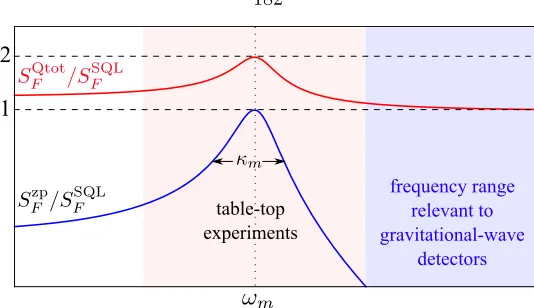
In Chapter 6, we provide an alternative viewpoint to Ref. [62], by emphasizing more the role of quantum back-action and its relation to the quantization of the mechanical oscillator. First of all, we separate the experimental system into two parts. The cooling mode, the mechanical oscillator, and the environmental thermal bath couples to together forms the first part, which can be viewed as providing aneffective mechanical oscillatornearly at the ground state, but with a quality factor significantly lower than the intrinsic quality factor of the mechanical mode. It is the zero-point fluctuation of this effective oscillator that we shall be probing. The second part of the system consists of the readout mode, which couples to the effective oscillator (the first part of the system) through its displacement alone. The second part provides us with a probe-field output ˆy, which contains information about the zero-point fluctuation of the effective mechanical oscillator.

Using linear quantum measurement theory, we show that the output spectra Syy for the two

opposite detunings, ∆ =±ωm, are different from each other:

Syy(ω)|∆=−ωm =6 Syy(ω)|∆=ωm. (1.22)

This difference can be traced back to the correlation that exists between the sensing noise and the back-reaction noise. This correlation in turn arises from the quantum coherence between the mechanical oscillator and the measuring device, which builds up during the measurement process. As earlier works had indicated, the correlation between sensing noise and back-action noise is key to improving sensitivities beyond the standard quantum limit. As a consequence, this experiment with nanomechanical oscillators demonstrates a effect much sought after by the gravitational-wave-detection community.

(33)

1.2.5

Macroscopic quantum mechanics in a classical spacetime (Chapter

7)

Chapter 7 is based on the research paper published as:

• Huan Yang, Haixing Miao, Da-Shin Lee, Bassam Helou, Yanbei Chen,Macroscopic Quantum Mechanics in a Classical Spacetime, Physical Review Letters,110, 170401 (2013).

1.2.5.1 Motivations and significance

This work was initiated by Chen, who was thinking about the problem of scalar waves propagating in a curved spacetime. He later realized that it was also a model for quantized matter coupled with a classical spacetime, and urged me to think about the non-relativistic limit of this model and the possibility of testing it with experiments. We analyzed the non-relativistic evolution equation of a many-particle system in this model, and showed that the center-of-mass (CM) evolution can be singled out from evolution of internal degrees of freedom — this enabled us to derive the evolution equation for CM alone, which can be monitored and manipulated at quantum levels by state-of-the-art optomechanics experiments. We further showed that mass concentration inside a crystal (around the lattice sites) makes the CM motion deviate from standard quantum mechanics at a level that might be visible by a carefully designed lab-scale optomechanics experiment.

Testing the nature of gravity is a prominent problem in modern physics. Apart from the standard formulation of linearized quantum gravity [68], which seems rather implausible to test in the lab, several signatures have been conjectured: (i) gravity decoherence[70–80], where gravity introduces decoherence to macroscopic quantum superpositions; (ii) modifications to canonical quantization motivated by the existence of a minimum length scale [81–83], and (iii)semiclassical gravity[84–86], which will be the subject of this chapter. As originally suggested by Møller [84] and Rosenfeld [85], spacetime structure mightstill remain classicaleven if it is sourced by matters of quantum nature, if we impose (G=c= 1):

Gµν = 8πhψ|Tµνˆ |ψi. (1.23)

Here Gµν is the Einstein tensor of a (3+1)-dimensional classical spacetime, ˆTµν is the operator

for the energy-stress tensor, and |ψ(t)i is the wave function of all matters that evolve within this classical spacetime.

(34)

many-particle SN equation, obtained by Diosi and Penrose [69, 73], can be written as

i~∂tϕ=

X

k

−~

2_∇2

k

2mk +

mkU(t,xk)

2

ϕ+V(X)ϕ , (1.24)

whereV(X) is the potential energy for non-gravitational interactions, while the Newtonian potential

U is given by

∇2_U₍_t,_x_{) = 4}_πX j

Z

d3nX|ϕ(t,X)|2_mj_δ₍_x₋_x

j). (1.25)

Many-particle wave-functions are generally very fragile and difficult to model. Previously, it was proposed to test the above equation in the single-particle case [86]. However, in order to satisfy the single-particle approximation, the object’s size has to be smaller than the width of its wave function. This requirement limits the mass of the object and hence the gravitational interaction energy. In addition, the dynamical and decoherence timescales for a small object are usually too short compared with its gravitational interaction timescale. As a result, it is very difficult for single particle tests to achieve the desired sensitivity.

In Chapter 7, we show that it is possible to single out CM evolution from other degrees of freedom (DOFs) for a macroscopic object with many particles. Moreover, in certain parameter regimes, the CM wavefunction approximately satisfies the following SN equation:

i~∂Ψ

∂t =

−~

2_∇2 2M +

1 2M ω

2 CMx

2₊1 2M ω

2

SN(x− hxi) 2

Ψ. (1.26)

Here hxi ≡ hΨ|x|ˆΨi is the expectation value of the CM position; ωCM is the eigenfrequency in absence of gravity, determined by how the CM is confined; andωSNis a characteristic frequency due to the self-gravitational effect, which depends on material properties and temperature. For silicon crystal at low temperatures,ωSN is approximately∼0.036s−1.

Using the CM Schr¨odinger-Newton equation (7.2), we solve the equations of motion for the first (hxi,hpi) and second (Vxx, Vpp, Vxp) moments of position and momentum, and find they oscillate at different frequencies. The mean position and momentumhxi,hpi, which carry classical information about the object, remain oscillating at frequency ωCM; the seconds moments, or more precisely the noise ellipse, which is related to quantum uncertainties, oscillates at a new frequency ωq = p

ω2 SN+ω

2

(35)

radiation pressure noise to be comparable to thermal noise, and the separation between those two peaks to be smaller than the peak width. The latter requirement is equivalent to

Q>

∼ (ωCM/ωSN)2. (1.27)

For oscillators made from silicon crystals with ωSN ≈ 0.036 s−1, if ωCM ≈ 2π×10 Hz, Eq. (7.24) requires Q>

∼ 3×106, which is challenging but possible [87]. If a lower-frequency oscillator, e.g., a

torsional pendulum withωCM ≈2π×0.1 Hz [88] can be probed with back-action noise comparable to thermal noise, in that case we only requireQ>

∼3×102.

By analyzing the CM motion of a macroscopic object under classical gravity, we have demon-strated: (i) A model in which classical theory interfaces with a quantum theory. (ii) Optomechanics for macroscopic object is the regime (probably the only known so far) in which both self-gravitational effect and quantum effect are important. (iii) It is experimentally possible to use CM motion of a macroscopic oscillator to test semiclassical gravity or more specifically the non-relativistic limit of Eq. (7.1).

I performed the derivation of the CM Schr¨odinger-Newton equation, while Chen greatly refined my error estimates. I also wrote the initial draft of the paper, which was revised by Miao and Chen, with a number of useful suggestions from Lee.

1.3

Black hole perturbation theory

1.3.1

Background

Many gravitational-wave-emitting processes end with the formation of a black hole. For example, in the final stage of a binary black-hole merger, the spacetime is approximately a perturbed Kerr spacetime. The metric perturbations gradually radiate to infinity or get absorbed by the black hole, and eventually the whole spacetime settles down to a Kerr spacetime. In the past, various analytical tools were developed to describe the evolution of a perturbed black holes’s spacetime.

(36)

These results were further generalized by Moncrief, who recombined these 10 metric quantities to obtain 2 independent gauge invariant quantities. He also derived separated evolution equations for them:

∂2_ψ p

∂t2 −

∂2_ψ p

∂r2

∗

+Vpψp= 0. (1.28)

Here r∗=r+ 2Mlog(r/2M−1) and pcorresponds to the parity of the field. ψp are the gauge invariant quantities with even or odd parity and the potential terms Vp are given in Chapter 8. In addition, the horizon is located atr= 2M orr∗ =−∞, whereas spatial infinity is atr = +∞ or

r∗= +∞. .

Kerr black holesdo not have spherical symmetry. There is as yet no way to write down a single wave equation with separable angular and radial/time dependence which can be used to generate all other metric perturbations. However, Teukolsky managed to show [26] that certain components of curvature perturbations on the Kerr background obey separable wave equations in the frequency domain (the wave equations are listed in Chapters 10–12). In particular, these curvature quantities are the Newman-Penrose (NP) curvature scalars Ψ0 and Ψ4[27], both of which are gauge invariant under infinitesimal gauge transformations at linear perturbative order. Physically speaking, the quantity Ψ0originates from gravitational waves that go into the black horizon, whereas Ψ4originates from gravitational waves that radiate towards infinity. As a result, it is convenient to apply Ψ4 in numerical relativity simulations for wave extraction at infinity. In addition, with certain gauge choices, algorithms have been developed to reconstruct full metric perturbations from Ψ0 and Ψ4. For example, Chrzanowski [28], Kegeles and Cohen [29], Stewart [30] and Wald [31] demonstrated the metric reconstruction procedure in ingoing and outgoing radiation gauges. For systems with quasi-periodic dynamics and adiabatic evolution (such as Extreme Mass Ratio Inspiral or EMRI in Kerr spacetime), frequency domain analysis is accurate and much more efficient than time-domain methods. In those cases, the Teukolsky formalism becomes very useful. In other cases, however, where the adiabatic approximation does not hold or the frequency domain method is not accurate enough, we still need to solve coupled wave equations for the 10 metric perturbation quantities in order to determine the system’s evolution.

Although the perturbations of a Kerr black hole generically decay in time (see [32] for the proof of Kerr spacetime’s linear stability), these perturbations can still be decomposed into eigenmodes, each with a complex eigenfrequency. These eigenmodes are usually referred asQuasinormal Modes

(37)

Schwarzschild perturbation, this is equivalent to requiringψe/o∝e−iωln(t+r∗) whenr∗→ −∞, and

ψe/o∝e−iωln(t−r∗) whenr∗→ ∞. With these boundary conditions Eq. (1.28) can be solved in the

frequency domain. There are a series of eigenmodes, which are indexed by angular numberl and overtonen. Their frequenciesωln are complex numbers with negative imaginary parts. This agrees with [32] becauseωI with positive imaginary parts corresponds to growing or unstable modes.

For Kerr black holes the boundary condition at horizon has to be modified to take into account frame dragging effect. Ψ4 becomes (see Chapter 10 for more details)

Ψ4∝ 1 r5e

−i(ωlmn−mω+)(t+r∗)_, _r

∗→ −∞,

∝1 re

−iωlmn(t−r∗)_, _r

∗→+∞ (1.29)

and Ψ0becomes

Ψ0∝1 re

−i(ωlmn−mω+)(t+r∗)_, _r

∗→ −∞,

∝ 1 r5e

−iωlmn(t−r∗)_, _r

∗→+∞ (1.30)

where ω+ = M a/(2r+) is the horizon frequency, a = J/M is the black hole’s spin parameter and r+ = M +

√

M2₋_a2 _{is the outer-horizon radius. Similar to the Schwarzschild case, a series} of eigenmodes can be obtained by combining the Teukolsky equation Eq. (1.28) with boundary conditions in Eq. (1.29). Since Kerr black holes do not have spherical symmetry, the degeneracy of azimuthal degrees of freedom is broken and Kerr QNMs are indexed byl, nand azimuthal numberm. In generalωlmns are complex numbers with negative imaginary frequencies, with a few exceptions

for extreme Kerr black holes (a=M).

1.3.2

First-order perturbative Hamiltonian equations of motion for a

point particle orbiting a Schwarzschild black hole (Chapter 8)

Chapter 8 is based on the following preprint:

• Huan Yang, Haixing Miao, Yanbei Chen, First-Order Perturbative Hamiltonian Equations of Motion for a Point Particle Orbiting a Schwarzschild Black Hole, arXiv:1211.5410 [gr-qc].

(38)

wave equations can be naturally derived from the Hamilton-Jacobi equations, and the gauge choices are no longer limited to Lorenz gauge. Our Hamiltonian formalism allows more flexible gauge choices than other approaches, and introduces more efficient evolution schemes.

Simulating Extreme Mass Ratio Inspirals (EMRIs) is one of the outstanding problems in gravitational physics. A EMRI system often includes a supermassive black hole and an object with much smaller mass. EMRI is astrophysically interesting because a supermassive black hole is believed to exist in every galaxy; it is also conceptually intriguing because black-hole perturbation theory can be naturally applied here. However, computationally this is a difficult problem for numerical relativity simulations because of the large separation in length scales. Even in terms of black-hole perturbation theory, since the small mass object is often approximated as a point mass to avoid dealing with its equation of state, a special regularization procedure has to be performed to remove metric singularities on the point mass’s worldline.

The most common approach for metric regularization was developed by Detweiler and Whiting [90, 91]. The basic idea is to separate the metric perturbationhinto a regular piecehRand a singular

piece hS. The singular piece diverges at the particle’s location but does not have any effect on the

particle’s motion; it can be obtained by a local expansion of the Green function. The regular field satisfies the homogeneous Einstein’s equation and is responsible for the geodesic deviation of the particle’s motion in the background spacetime; it is obtained by subtracting the singular field from the full field. Using this regularization technique, there are two major approaches for numerically evolving the test particle and the metric perturbation. One way is themode sumapproach, developed by Barack and Ori [92], which decomposes each of the 10 metric components into spherical harmonics, and solves 10 coupled 1+1 wave equations for each (l, m). The particle equation of motion is then regularized mode-by-mode, by subtracting a series of regularization parameters for each (l, m). This mode sum method has already been implemented by Warburton et al. [93] for the Schwarzschild gravitational EMRI problem. In the second approach, one directly applies a 3+1 decomposition of spacetime geometry, and tries to obtain the regular field directly — by obtaining a field ˜hR which is

approximately the Detweiler-Whiting hR near the particle, but gradually becomes the full field at null infinite and near horizon. As shown by Vega and Detweiler [94], the field ˜hR satisfies a wave equation with out-going boundary condition at infinity and horizon, but with a source that can be computed from the Detweiler-Whiting singular field hS. Diener and Vega [95] have implemented this method for a scalar particle orbiting a Schwarzschild black hole.

(39)

a spherically decomposed 1+1 scheme. Following the work of Moncrief, we write down an action for perturbations in space-time geometry, combine that with the action for a point-particle moving through this space-time, and then obtain Hamiltonian equations of motion for metric perturba-tions and the particle’s coordinates, as well as their canonical momenta. Hamiltonian equaperturba-tions for the metric-perturbation and their conjugate momenta, for even and odd parities, reduces to Zerilli-Moncrief and Regge-Wheeler master equations with source terms, which are gauge invariant, plus auxiliary equations that specify gauge. Hamiltonian equations for the particle, on the other hand, now include effect of metric perturbations — with these new terms derived from the same interaction Hamiltonian that had lead to those well-known source terms. In this way, space-time geometry and particle motion can be evolved in a self-consistent manner, in principle in any gauge. However, the point-particle nature of our source requires regularization, and we outline how the Detweiler-Whiting approach can be applied. In this approach, a singular field can be obtained ana-lytically using the Hadamard decomposition of the Green’s function; while the regular field, which needs to be evolved numerically, is the result of subtracting the singular field from the total metric perturbation. In principle, any gauge that has the singular-regular field decomposition is suitable for our self-consistent scheme. In reality, however, this freedom is only possible if our singular field has a high enough level of smoothness. For a singular field with minimum quality, one can adopt the Lorenz gauge condition, which we have recast into our formalism: for eachl andm, we have 2 wave equations to evolve odd and even parity gauge invariant quantities and 8 first order differential equations to fix the Lorenz gauge and determine all the metric components.

I performed most of the analytical calculations in this work, and also wrote the initial version of the paper, which was greatly revised by Chen.

1.3.3

Quasinormal mode spectrum of Kerr black holes and its geometric

interpretation (Chapter 9)

Chapter 9 is a research paper published as:

• Huan Yang, David A. Nichols, Fan Zhang, Aaron Zimmerman, Zhongyang Zhang, and

Yan-bei Chen, Quasinormal-mode spectrum of Kerr black holes and its geometric interpretation, Physical Review D86104006 (2012).

(40)

analytical understanding for Kerr QNM frequency is needed. We worked out the QNM frequency formula in the eikonal limitl1 using WKB techniques, which agrees with numerical results very well. Using the analytical formula, the mode degeneracies are naturally explained and moreover, we showed these Kerr QNMs are intimately related to null particles moving in spherical orbits of

Topics in Gravitational-Wave Science: Macroscopic Quantum Mechanics and Black Hole Physics