Advance Access publication 2017 June 14
Stable habitable zones of single Jovian planet systems
Matthew T. Agnew,
1‹Sarah T. Maddison,
1Elodie Thilliez
1and Jonathan Horner
2 1Centre for Astrophysics and Supercomputing, Swinburne University of Technology, Hawthorn, Victoria 3122, Australia2University of Southern Queensland, Toowoomba, Queensland 4350, Australia
Accepted 2017 June 8. Received 2017 June 6; in original form 2016 September 29
A B S T R A C T
With continued improvement in telescope sensitivity and observational techniques, the search for rocky planets in stellar habitable zones is entering an exciting era. With so many exo-planetary systems available for follow-up observations to find potentially habitable planets, one needs to prioritize the ever-growing list of candidates. We aim to determine which of the known planetary systems are dynamically capable of hosting rocky planets in their habitable zones, with the goal of helping to focus future planet search programmes. We perform an ex-tensive suite of numerical simulations to identify regions in the habitable zones of single Jovian planet systems where Earth-mass planets could maintain stable orbits, specifically focusing on the systems in the Catalog of Earth-like Exoplanet Survey Targets (CELESTA). We find that small, Earth-mass planets can maintain stable orbits in cases where the habitable zone is largely, or partially, unperturbed by a nearby Jovian, and that mutual gravitational interactions and resonant mechanisms are capable of producing stable orbits even in habitable zones that are significantly or completely disrupted by a Jovian. Our results yield a list of 13 single Jovian planet systems in CELESTA that are not only capable of supporting an Earth-mass planet on stable orbits in their habitable zone, but for which we are also able to constrain the orbits of the Earth-mass planet such that the induced radial velocity signals would be detectable with next generation instruments.
Key words: astrobiology – methods: numerical – planets and satellites: dynamical evolution and stability – planets and satellites: general.
1 I N T R O D U C T I O N
One of the most exciting goals in astrophysics is the discovery of a true, twin Earth: a rocky planet of similar size, structure and com-position to Earth on a stable orbit within its host star’s habitable
zone1(HZ) (Kasting, Whitmire & Reynolds1993; Kopparapu et al.
2013). As a result of biases inherent to observational techniques,
the first exoplanets detected were often both massive and close to
their host stars (e.g. Mayor & Queloz 1995; Charbonneau et al.
2000). In the decades since, improved technology has allowed for
the detection of lower mass planets (e.g. Vogt et al.2015; Wright
et al.2016) and planets with greater orbital periods (e.g. Borucki
et al. 2013; Jenkins et al. 2015). We are only now beginning to
discover planets with orbital periods of a decade or more,
includ-ing Jupiter analogues (Wittenmyer et al.2016). We now know of
over 34002confirmed exoplanets (NASA Exoplanet Archive,
E-mail:magnew@swin.edu.au
1The HZ is a region around a star in which liquid water can be maintained on the surface of a rocky planet that hosts an atmosphere.
2As of 2017 February 2.
planetarchive.ipac.caltech.edu) with a variety of radii, masses and orbital parameters. In the coming years, we will begin to search for potentially habitable exo-Earths and so in this work we aim to determine how to best focus our future efforts.
Several methods have been used in the past to predict stable regions and the presence of additional exoplanets in confirmed ex-oplanetary systems. Some methods predict the presence of a planet by simulating observable properties of debris discs (e.g. Thilliez &
Maddison2016). Others utilize dynamical simulations to
demon-strate that massless test particles (TPs) can remain on stable orbits in multiple planet systems, thus identifying potential regions of
stability (e.g. Rivera & Haghighipour2007; Thilliez et al.2014;
Kane2015). Such stable regions can then be the focus of follow-up
simulations involving Earth-mass planets (Kane2015).
Assessing the stability of a system by considering a region of chaos surrounding any known exoplanet has also been used to pre-dict regions of stability in exoplanetary systems (Jones, Sleep &
Chambers2001; Jones & Sleep2002; Jones, Underwood & Sleep
2005; Jones & Sleep2010; Giuppone, Morais & Correia2013).
The unstable, chaotic region around a planet is often calculated
to be some multiple of its Hill radius (Jones et al.2001; Jones &
Sleep2002), where the multiplying factor is sometimes derived
Table 1. The distribution of exoplanets between Terrestrial planets, Super-Earths, Neptunians and Jovians amongst sin-gle and multiple planet systems. The class of each planet is defined by Table2.
Single Multiple Total
Terrestrials 320 304 624
Super-Earths 458 431 889
Neptunians 349 308 657
Jovians 601 152 753
Total 1728 1195 2923
numerically (Jones et al.2005; Jones & Sleep2010). Alternatively,
Giuppone et al. (2013) present a semi-empirical stability criterion
to quickly infer the stability of existing systems. They test the va-lidity of the criterion by simulating both single and multiple planet systems, and demonstrate that their criterion is an effective tool for identifying which exoplanetary systems can host additional planets. In this work, we aim to identify the properties of planetary archi-tectures in single Jovian planet systems that could harbour an Earth-mass planet in the HZ, with a specific focus on those presented in the Catalog of Earth-like Exoplanet Survery Targets (CELESTA;
Chandler et al.2016). We first divide the selected systems into three
broad classes that indicate their likelihood of hosting stable Earths in their HZs in order to theoretically eliminate systems that almost certainly host stable HZs from our numerical study. Since these HZs are all stable, numerical simulations would not help constrain the locations within the HZ where stable Earths might reside. For
the remaining systems, we use theSWIFTN-body software package
(Levison & Duncan1994) to help identify regions where Earth-mass
planets could maintain stable orbits by first performing dynamical simulations using the spread of massless TPs throughout the HZ of each system. We follow these with a suite of dynamical simulations
using a 1 M⊕planet to ultimately predict which systems could host
a stable Earth in their HZs, help constrain the orbits of the stable Earth, and determine what the strength of the induced radial velocity signal would be.
In Section 2, we introduce the motivation for analysing single Jovian planet systems. In Section 3, we describe the method used to select the single Jovian planet systems that we simulate, detail the numerical simulations used to dynamically analyse the systems and discuss how we interpret the simulation results. We then present and discuss our results in Section 4, and summarize our findings in Section 5.
2 E X O P L A N E T P O P U L AT I O N
Using the Exoplanet Orbit Database (Han et al.2014,
exoplan-ets.org), we analyse the currently known exoplanet population.3
Our analysis reveals an interesting feature: the proportion of Jovian planets in single and multiple planetary systems is skewed in favour
of single planet systems (see Table1). Single Jovian planet systems
are an interesting sub-set of the exoplanet population that could potentially have small rocky planets hidden in their HZs. Jupiter is thought to have played a complicated role in the formation and
evolution of the Solar system (e.g. Gomes et al.2005; Horner et al.
2009; Walsh et al.2011; Izidoro et al.2013; Raymond & Morbidelli
3It should be noted that there are inherent biases in the various observational techniques that may impact the following analysis, but for this work we accept the planetary properties and orbital parameters as they are in the relevant data bases.
Table 2. The radius and mass limits used in this work to classify exoplanets.
rmin rmax mmin mmax
(r⊕) (r⊕) (M⊕) (M⊕) Terrestrials 0 <1.5 0 <1.5 Super-Earths 1.5 <2.5 1.5 <10
Neptunians 2.5 <6 10 <50
Jovians 6 >6 50 >50
2014; Brasser et al.2016; Deienno et al.2016), although the
tim-ing, nature and degree to which it has contributed to is a dynamic
area of research (e.g. Minton & Malhotra2009,2011; Agnor & Lin
2012; Izidoro et al.2014, 2015, 2016; Levison et al.2015; Kaib
& Chambers2016). Further to this, it has also been suggested that
Jupiter may have had a significant impact on the environment in which life on Earth has developed (e.g. Bond, Lauretta & O’Brien
2010; Carter-Bond, O’Brien & Raymond2012a,b; Martin & Livio
2013; Quintana & Lissauer2014; O’Brien et al.2014). For this
rea-son, it has been proposed that the presence of a Jupiter analogue in an exoplanetary system may be an important indicator for potential
habitability (Wetherill1994; Ward & Brownlee2000), although this
hypothesis remains heavily debated (Horner & Jones2008,2009,
2010,2012; Horner, Gilmore & Waltham2015; Grazier2016).
Our analysis using the Exoplanet Orbit Database yields a total
of 29234exoplanets, residing in 2208 systems: 1728 single and
480 multiple planet systems. These exoplanets are classified as Ter-restrials, Super-Earths, Neptunians and Jovians according to their radius (or according to their mass in lieu of available radius data)
as per the ranges defined in Table2. Analysing all the exoplanet
systems, we find that the exoplanet classes are distributed amongst
the systems as shown in Table1. It can be seen that all classes of
planets are reasonably well represented not only within the greater exoplanet population, but also within the single and multiple planet sub-populations.
Of particular interest is an investigation into the planetary ar-chitectures of the multiple planet systems. We classify the 480 multiple systems into three broad categories based on the planet classes present in each: non-Jovian systems, Jovian systems that coexist with smaller Terrestrial or Super-Earth planets, and Jovians
and Neptunians with other giant planets. Fig.1(a) demonstrates that
when a multiple system is found harbouring a Terrestrial or
Super-Earth planet, in the majority of cases (343/480,∼71 per cent) it
coexists with other Terrestrial planets, Super-Earths or Neptunians.
Fig.1(b) shows that systems with Terrestrials or Super-Earths
co-exist with a Jovian account for the small fraction of the multiple
planet systems (16/480,∼3 per cent), while Fig.1(c) shows that
non-Terrestrial or Super-Earth systems account for about a quarter
(121/480,∼25 per cent) of the multiple planet systems. While the
overall distribution of planets in multiple planet systems shows a
reasonable distribution across each class (Table1), the planet classes
are not uniformly distributed in each multiple planet architecture: Terrestrial planets and Super-Earths are generally found with other Terrestrials, Super-Earths or Neptunians, whereas Jovians are gen-erally found with other massive planets, i.e. Neptunians and/or Jo-vians.
Examining the entire Jovian population as they occur in both single and multiple systems yields a total of 753 planets. We summarize our findings concerning Jovians as follows: 601
4Confirmed exoplanets for which good orbital elements and mass and/or radius data are available as of 2017 February 2.
[image:2.595.70.263.103.182.2]Figure 1. Planetary architectures of confirmed multiple planet systems. The exoplanets have been classified as per the criteria presented in Table2. (a) The 343 multiple planet systems with Terrestrial planets or Super-Earths that also do not possess a Jovian. (b) The 16 multiple planet systems with Terrestrial planets or Super-Earths that also do possess a Jovian. (c) The 121 multiple planet systems with no Terrestrial planets or Super-Earths.
(79 per cent) Jovians are found in single planet systems, 128 (17 per cent) Jovians are found in multiple planet systems coex-isting with Neptunians or other Jovians and only 24 (3 per cent) Jovians are found in multiple planet systems coexisting with Ter-restrial planets or Super-Earths. This demonstrates that for the cur-rent population of confirmed exoplanets, the majority of Jovians are either found to be in single planet systems or to coexist with other giant Jovians or Neptunians, contrasting with our own So-lar system. However, we note that this is most likely attributable to observational bias inherent in the two highest yield detection methods: the transit method and radial velocity method. The cur-rent state of the art allows for the detection of Doppler shifts to
just below 1 m s−1(Dumusque et al.2012), making the detection of
Earth-mass planets challenging (Wittenmyer et al.2011). As such,
Jovians will completely dominate both Doppler shift signals and transit signals. The detection of Terrestrials in the HZs of Sun-like stars is even more challenging because such planets would orbit within a few au of their host stars. The next generation of spec-trographs aim to detect such planets by achieving radial velocity
resolutions of around 0.1 m s−1(e.g. ESPRESSO; Pepe et al.2014)
and 0.01 m s−1(e.g. CODEX; Pasquini et al.2010). As the radial
velocity resolution decreases, the resultant noise from the stellar
ac-tivity in Sun-like stars becomes significant (Dumusque et al.2011a;
Anglada-Escud´e et al.2016). We do not consider stellar noise in
our assessment herein. The small proportion of Jovians coexisting with rocky planets and the observational biases inherent to the cur-rent state of the art provides motivation to investigate single Jovian planet systems as a sub-set of the existing exoplanet population which may contain smaller Terrestrial planets in the HZ which are currently undetectable.
Giuppone et al. (2013) briefly discuss the idea of multiple planets
in tightly packed configurations called compact systems. In such a system, all possible stable regions are occupied, and the system can
be considered full; no additional bodies can exist on stable orbits. An excellent example of such a compact multiple planet system is the recently announced seven planet system detected orbiting
TRAPPIST-1 (Gillon et al.2017). While single Jovian planet
sys-tems are clearly not compact, their HZs may be full, depending on the orbital parameters of the existing Jovian. It is important to determine which systems have full HZs in order to eliminate those systems as possible targets for future observations in the search for potentially habitable Earth-like planets.
In this work, we aim to investigate the sub-set of these single
Jovian planet systems that are in CELESTA (Chandler et al.2016).
The CELESTA data base calculates the HZs of nearby Sun-like stars, calculating the stellar properties needed to determine the HZs
from Kopparapu et al. (2014), and presents several possible HZ
boundaries to choose from. As a large proportion of the exoplanet population is observed around non-Sun-like stars (e.g. M-dwarfs), the data base does not contain many stars with planetary bodies. Of the 37 354 stars in CELESTA for which HZs are calculated, just 120 host confirmed exoplanets. Of these 120, just 93 are single Jovian planet systems. We cross reference these systems from CELESTA
with the Exoplanet Orbit Database (Han et al.2014) to yield the
planetary properties and orbital parameters. In this work, we aim to
identify which of these systems could host a 1 M⊕planet in a stable
orbit within the HZ. For these systems, we then determine those for which such a planet could be detected using future instruments, in order to provide a focus for future observational efforts.
3 M E T H O D
We first calculate a theoretical region of chaos surrounding the existing Jovian in the selection of 93 CELESTA systems. To save simulation time, we remove systems that have completely stable HZs. While these systems could host stable Terrestrial planets in
their HZs, we cannot offer any further constraints on the orbits of such habitable planets. For the remaining systems, we first carry out dynamical simulations using the spread of massless TPs throughout the HZ of each system to help identify regions of dynamical stability in the HZ. For those systems predicted to have less stable HZs, we expect significantly more interactions between TPs and the Jovian, and potentially some resonant trapping. We increase the number of TPs for these systems in order to yield more robust results. Finally,
we conduct a suite of simulations involving the Jovian and a 1 M⊕
planet to check if mutual gravitational interactions (that are absent with massless TP simulations) affect any stable regions found in the TP simulations in order to demonstrate where Terrestrial planets could be stable in those systems.
3.1 System selection
Here, we present the method used to broadly predict the overall stability of the HZs of exoplanetary systems. In the cases where the Jovian is located sufficiently far from the HZ, we expect the gravitational influence of the Jovian to be negligible on the HZ and leave it completely unperturbed. TPs within such an HZ would be capable of maintaining stable orbits and so are computationally expensive to run and provide little value, and so we want to eliminate such systems before proceeding with our numerical study.
We consider the criterion for the onset of chaos based on the
over-lap of first order mean-motion resonances (Wisdom1980; Duncan,
Quinn & Tremaine1989). For a planet orbiting its parent star, a
re-gion extending a distanceδaround the planet will experience chaos,
which is given by
δ=Cμ2/7aplanet,
(1)
whereCwas calculated to be a constant equal to 1.57 (Duncan
et al.1989; Giuppone et al.2013),μ=Mplanet/M∗is the mass ratio
between the planet and its parent star andaplanetis the semimajor
axis of the Jovian planet. Using this overlap criterion for the onset of
chaos, Giuppone et al. (2013) present thecrossing orbits criterion,
which suggests that if two planetary orbits intercept at some point, and in the absence of some kind of resonant mechanism, close encounters will occur and the system will become unstable. For a Jovian planet with an eccentric orbit, the chaotic region will extend
to a distanceδexterior to the apocentre and interior to the pericentre
of its orbit. Thus, the region of chaos is defined as
aplanet(1−e)−δ≤Chaotic Region≤aplanet(1+e)+δ, (2)
where e is the Jovian’s eccentricity and δ is defined as in
equation (1).
We use equation (2) to calculate the region of chaos for each of the 93 single Jovian systems from the CELESTA data base. We then compare the maximum and minimum semimajor axes of the chaotic region with the maximum and minimum semimajor axes of the HZ for each system, and compute the overlap between these two regions. From this, we define three classes of systems:
Green:if the chaotic region does not overlap the HZ. Amber:if the chaotic region partially overlaps the HZ.
Red:if the chaotic region completely overlaps the HZ.
We predict that the green non-overlapping systems should possess entirely stable HZs, the amber partially overlapping systems should possess partially stable HZs and the red completely overlapping systems should possess unstable HZs, except where the mutual gravitational interactions between the two bodies could stabilize
[image:4.595.308.550.102.196.2]specific orbits (as per the definition by Giuppone et al.2013). We
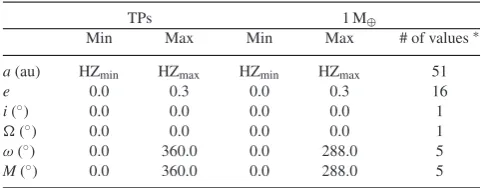
Table 3. The range of orbital parameters within which the TPs were ran-domly distributed over the HZ and the range of orbital parameters, and number of values over each range (in equally spaced intervals) over which the 1 M⊕body simulations were run.
TPs 1 M⊕
Min Max Min Max # of values∗
a(au) HZmin HZmax HZmin HZmax 51
e 0.0 0.3 0.0 0.3 16
i(◦) 0.0 0.0 0.0 0.0 1
(◦) 0.0 0.0 0.0 0.0 1
ω(◦) 0.0 360.0 0.0 288.0 5
M(◦) 0.0 360.0 0.0 288.0 5
find that for the 93 single Jovian planet systems, 41 can be classified as green, 26 as amber and 26 as red. We focus our attention on the red completely overlapping systems and amber partially overlapping systems, where the influence of the Jovian is predicted to strongly or relatively strongly influence the HZ. As the green non-overlapping systems are predicted to have stable HZs and are expected to retain the majority, if not all, of their TPs, simulations would not help constrain the orbits of potentially habitable Terrestrial planets in those systems. Thus, we focus on only those green systems where the Jovian is close to the HZ; that is, where the period of the Jovian,
TJovian, is within one order of magnitude of the period in the HZ
centre, THZ (0.1THZ ≤TJovian ≤10THZ). There are 13/41 green
systems that satisfy this criterion.
3.2 Dynamical simulations
We run dynamical simulations using the SWIFT N-body software
package (Levison & Duncan 1994).SWIFT can integrate massive
bodies that interact gravitationally, and massless TPs that feel the gravitational forces of the massive bodies but exert no gravitational force of their own. We use the regularised mixed variable symplectic
(RMVS) method (specifically, thermvs3integrator) provided in
SWIFT due to its advantage of being computationally faster than
conventional methods (Levison & Duncan2000).
We used the Runaway Greenhouse and Maximum Greenhouse
scenarios presented by Kopparapu et al. (2014) for the inner and
outer edges of the HZ, respectively.5The inner edge corresponds
with the maximum distance from the star at which a runaway green-house effect would take place, causing all the surface water on the planet to evaporate. The outer edge corresponds to the maximum
distance at which a cloud-free CO2atmosphere (with a background
of N2) could maintain liquid water on the Terrestrial planet’s surface.
The Runaway Greenhouse and Maximum Greenhouse boundaries make up the conservative HZ. The HZ boundaries have been shown to be strongly dependent on the uncertainties in stellar parameters
(Kane2014). In this work, however, we take the stellar parameters
given in CELESTA and the Exoplanet Orbit Database on face value. The TPs were then randomly distributed throughout the HZ, within
the range of orbital parameters shown in Table3. All simulations
used stellar parameters and HZ values from CELESTA (Chandler
et al.2016), and planetary properties and orbital parameters from
the Exoplanet Orbit Database (Han et al.2014).
The simulations were run for an integration time Tsim = 107
yr or until all the TPs were removed. The removal of a TP is defined by the ejection of the TP beyond an astrocentric distance of
5Assuming an Earth-mass planet and an Earth-like atmosphere.
Table 4. A description and size of the sets of simulations run as part of our simulation suite.
Set Description
I A set of 13 simulations with 1000 TPs in the HZ for all green non-overlapping systems where the orbital period of the Jovian was within one order of magnitude of the period in the centre of the HZ (0.1THZ≤TJovian≤10THZ).
II A set of 26 simulations with 5000 TPs in the HZ for all amber partially overlapping systems.
III A set of 26 simulations with 10 000 TPs in the HZ for all red completely overlapping systems.
IV A set of 20 400 simulations with a 1 M⊕planet for the 26 red completely overlapping systems (530 400 simulations in total). For each system, 20 400 simulations were run, sweeping a 1 M⊕ planet over the orbital parameter space as outlined in Table3. V A set of 20 400 1 M⊕planet simulations for those red systems
that are found to be stable in a narrow region of resonant stability (15/26 systems) for a simulation timeTsim=108yr.
250 au. The time-step for the simulations was set to dt=1/40 of
the smallest orbital period in the system (Jovian planet or TPs).
Table4describes the sets of simulations that were carried out. Set
I tests the sub-set of the green non-overlapping systems that have their Jovians nearest to their respective HZs. Set II tests the amber partially overlapping systems with 5000 TPs and set III tests the red completely overlapping systems with 10 000 TPs. Increasingly more TPs were used for those systems with predictably more inter-acting HZs to achieve higher resolution maps when analysing the results.
Simulation set IV comprises a suite of simulations for each red
completely overlapping system with a 1 M⊕planet in the HZ, along
with the system’s Jovian. Assuming co-planar planets, these
simu-lations explored the semimajor axis (a), eccentricity (e), argument
of periastron (ω) and mean anomaly (M) parameter space of the
1 M⊕planet. Table3shows the range of orbital parameters and the
number of equally spaced intervals within each range. In total, a suite of 20 400 simulations were carried out for each system, with each simulation representing a unique set of planetary orbital
pa-rameters. As there are five values explored for bothωandM, this
means that there are 25 simulations for a given pair of (a,e) values.
The 1 M⊕simulations were ran forTsim=107yr, or until one of
the planets was removed or was involved in a collision. As all the Jovian planets in these red completely overlapping sample were located in the vicinity of the HZ (which was located well within 10 au), a planet removal was defined following Robertson et al.
(2012): if either planet exceeded an astrocentric distance of 10 au.
A collision was defined as occurring when the planets approached
within 1 Hill radii of each other. The time-step for these 1 M⊕
sim-ulations was set to 1/20 of the smallest orbital period of the Jovian
and 1 M⊕ planet. Simulation set V repeats these 1 M⊕ body
sim-ulations for red systems which hosted some stable regions for an
extended integration time ofTsim=108yr.
3.3 Simulation analysis
The results of the simulations were interpreted using stability maps and resonant angle plots. The stability maps are plotted over
the semimajor axis–eccentricity (a,e) parameter space. This
two-Figure 2. A comparison between the stability maps for the simulations of (a) 10 000 TP in the HZ and (b) the 20 400 1 M⊕simulations of the red completely overlapping system HD 137388. We mark the location of several first and second order MMRs with green dashed lines.
dimensional map presents the lifetimes of bodies as a function of
their initial semimajor axis (x-axis) and eccentricity (y-axis) values.
For the Earth-mass planet simulations (sets IV and V), each
simulation had the 1 M⊕ planet at a specified initial (a, e). As
mentioned above, at each (a,e) position, there are 25 simulations
exploring the (ω,M) parameter space. As such, the maps combine
the results of the 25 simulations over the (ω,M) parameter space
by plotting the mean lifetime of all bodies with those (a,e) values
(similar to previous work by Robertson et al.2012; Wittenmyer,
Horner & Tinney2012). Fig.2shows a comparison of the two
types of stability maps: the lifetime of randomly distributed TPs
across the HZ (Fig.2a) and the average lifetime of a 1 M⊕ body
being swept through the orbital parameter space (Fig.2b).
Fig. 3 shows the time evolution of the resonant angle for all
1 M⊕ bodies that were trapped in 4:3 resonance with the Jovian
planet in the HD 137388 system from our simulations. Such plots
reveal whether potentially resonant 1 M⊕ bodies librate, and can
therefore be considered to be trapped in mean-motion resonance (MMR).
Figure 3. The librating resonant angleφ=4λ−3λ−ωversus time for the stable bodies (6) of the 4:3 MMR with the Jovian in the red completely overlapping system HD 137388. Note that each body is run in its own simulation, with the resonant angle from all simulations stacked.
Figure 4. The stability map of the green non-overlapping system HD 67087 with 1000 TPs in the HZ. The Jovian planet is located interior to the HZ. We mark the location of several first and second order MMRs with green dashed lines.
4 R E S U LT S A N D D I S C U S S I O N
For the green non-overlapping systems where the orbital period of the Jovian was within one order of magnitude of the period in the centre of the HZ which we simulated in set I, we found that some TPs in the HZ were still disrupted by the presence of
such a Jovian. An example system is shown in Fig.4. Despite this,
our results demonstrated that the majority of the TPs remain in stable orbits in the HZ. As a result of their stability, these systems were computationally expensive to simulate, since typically they retain the majority, if not all, of their TPs. Due to the presence of these large, unperturbed regions of the HZ within which TPs are dynamically stable, we conclude that it is dynamically possible for a Terrestrial planet to be hidden in the HZ of green non-overlapping systems for which the chaotic region does not overlap the HZ. Given that we cannot further constrain the location of these potentially habitable Terrestrials, the green systems were not tested further.
[image:6.595.308.549.58.241.2]Based on the classification and selection scheme outlined in Sec-tion 3.1, the results from the amber partially overlapping systems
Figure 5. The stability map of the the amber partially overlapping system HD 48265 with 5000 TPs in the HZ. The Jovian planet is located interior to the HZ. We mark the location of several first and second order MMRs with green dashed lines.
(set II) behave as expected. We can see in Fig.5that there is a
gra-dient of stability across the HZ, moving from more stable regions farther from the Jovian to more unstable in regions nearer to the Jovian. Similar to the green non-overlapping systems, the presence of large, unperturbed regions of the HZ where TPs are dynamically stable in the amber partially overlapping systems suggest that it is dynamically possible for a Terrestrial planet to be hidden in the HZ of these systems. Our simulations cannot further constrain these locations, so no further investigation of these systems is conducted. More than half of the red systems were found to contain regions of stability, some of which were aligned with the MMRs of the Jovian. As the HZs of these systems were significantly influenced by the presence of the Jovian, it would be reasonable to consider whether mutual interactions with the massive planet affected the stability. We continued this investigation with additional simulations in which
we replaced the massless TPs with a 1 M⊕planet. Set IV examined
all 26 of the red completely overlapping systems and identified 15
systems for which 1 M⊕planets might prove stable at some location
within the HZ. For Set V, we took this sub-set of 15 stable systems
and performed significantly longer simulations of durationTsim=
108yr. The results showed that all 15 of these systems were found
to be capable of hosting a 1 M⊕ planet on a stable orbit within
their HZs, and were then reclassified as blue resonant systems.6
Fig. 6shows the stability maps of all 15 of these blue resonant
systems from set V, while Table5shows the system properties of
the 11 remaining red completely overlapping systems and the 15 reclassified blue resonant systems.
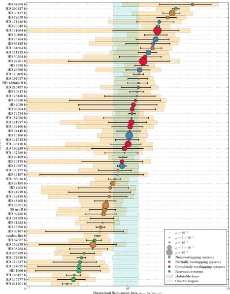
We next consider the architectures of all 65 systems we simulated.
Fig. 7plots normalized semimajor axis (a/aHZ,mid) along thex
-axis and all the systems along the y-axis in increasing order of
their normalized semimajor axis. The normalized semimajor axis indicates where an object is located relative to the centre of the HZ (aHZ, mid), and can also be used to indicate the locations of the inner
and outer boundaries of the HZ and chaotic region relative toaHZ,mid.
The advantage of the normalized semimajor axis is that it allows
6Note that this label is semantic, as it was found that some of the stable bodies do not appear to be in resonant configurations (stable bodies that are not in an MMR do not show up in the libration plots shown in Fig.A1).
[image:6.595.46.287.286.472.2]Figure 6. The stability maps for all the red systems with stable MMRs. These are the 15 systems re-classifed as blue resonant systems.
for a clearer comparison across systems. We plot the normalized semimajor axis for the position of the Jovian with error bars that represent the periastron and apastron of its orbit (so systems with larger error bars indicate a higher eccentricity), the HZ of each
system in aqua (the inner and outer edges) and the chaotic region of each Jovian in orange. Each Jovian is then plotted with a size
corresponding to its mass ratio,μ, and a colour corresponding to its
overlapping classification (green, amber, red or blue).
Table 5. The system properties and orbital parameters of the blue resonant (upper) and red completely overlapping (lower) systems. All Jovians were detected via the radial velocity method.
Star Jovian†
Type Mass HZinner HZouter Msini a e ω Instrument Detection reference∗
(M ) (au) (au) (MJupiter) (au) (◦)
HD 10697 G5 IV 0.847 1.735 3.116 6.23505 2.13177 0.099 111.2 HIRESa Vogt et al. (2000)
HD 16760 G5 V 0.991 0.7573 1.3407 13.2921 1.08727 0.067 232 HIRESa, HDSb Sato et al. (2009)
HD 23596 F8 1.19 1.5307 2.681 7.74272 2.77219 0.266 272.6 ELODIEc Perrier et al. (2003)
HD 34445 G0 V 1.06 1.425 2.5121 0.790506 2.06642 0.27 104 HIRESa Howard et al. (2010)
HD 43197 G8 V 0.945 0.8359 1.485 0.596868 0.918027 0.83 251 HARPSd Naef et al. (2010)
HD 66428 G5 0.83 1.254 2.257 2.74962 3.14259 0.465 152.9 HIRESa Butler et al. (2006)
HD 75784 K3 IV 0.719 2.408 4.4125 5.6 6.45931 0.36 301 HIRESa Giguere et al. (2015)
HD 111232 G5 V 0.933 0.8849 1.574 6.84182 1.97489 0.2 98 CORALIEe Mayor et al. (2004) HD 132563 B – 1.53 1.496 2.585 1.492470 2.62431 0.22 158 SARGf Desidera et al. (2011) HD 136118 F9 V 1.09 1.67 2.939 11.6809 2.33328 0.338 319.9 Hamiltong Fischer et al. (2002)
HD 137388 K0/K1 V 0.8819 0.6848 1.225 0.227816 0.88883 0.36 86 HARPSd Dumusque et al. (2011b)
HD 147513 G3/G5 V 1.109 0.9279 1.6312 1.179650 1.30958 0.26 282 CORALIEe Mayor et al. (2004)
HD 148156 F8 V 1.324 1.26 2.197 0.847612 2.12913 0.52 35 HARPSd Naef et al. (2010)
HD 171238 K0 V 0.955 0.89014 1.58 2.60901 2.54268 0.4 47 CORALIEe S´egransan et al. (2010)
HD 187085 G0 V 1.24 1.349 2.359 0.803694 2.02754 0.47 94 UCLESh Jones et al. (2006)
HD 216437 G2/G3 IV 1.102 1.4115 2.4825 2.16817 2.48556 0.319 67.7 UCLESh Jones et al. (2002)
HD 131664 G3 V 1.122 1.165 2.047 18.3282 3.17098 0.638 149.7 HARPSd Moutou et al. (2009)
HD 132406 G0 V 0.848 1.34 2.406 5.60495 1.98227 0.34 214 ELODIEc da Silva et al. (2007)
HD 141937 G2/G3 V 1.13 0.9993 1.755 9.4752 1.50087 0.41 187.72 CORALIEe Udry et al. (2002)
HD 16175 G0 1.15 1.749 3.069 4.37946 2.1185 0.6 222 Hamiltong Peek et al. (2009)
HD 190228 G5 IV 0.962 2.014 3.574 5.94193 2.60478 0.531 101.2 ELODIEc Perrier et al. (2003)
HD 2039 G2/G3 IV/V 1.16 1.399 2.453 5.92499 2.19755 0.715 344.1 UCLESh Tinney et al. (2003)
HD 22781 K0 V 0.83 0.58511 1.053 13.8403 1.16847 0.8191 315.92 SOPHIEi D´ıaz et al. (2016) HD 45350 G5 V 0.999 1.176 2.081 1.83614 1.94413 0.778 343.4 HIRESa Marcy et al. (2005) HD 50554 F8 V 1.18 1.103 1.9319 4.39876 2.26097 0.444 7.4 HIRESa, Hamiltong Fischer et al. (2002) HD 86264 F7 V 1.4 1.866 3.245 6.62738 2.84117 0.7 306 Hamiltong Fischer et al. (2009) †I,andMwere 0.0◦for all systems simulated.
∗Detection reference from the Exoplanet Orbit Database (Han et al.2014).
aHigh Resolution Echelle Spectrometer (HIRES) at Keck Observatory. bHigh Dispersion Spectrograph (HDS) at the Subaru Telescope. cELODIE echelle spectrograph at the Haute-Provence Observatory.
dHigh Accuracy Radial velocity Planet Searcher (HARPS) spectrograph at La Silla Observatory. eCORALIE echelle spectrograph at La Silla Observatory.
fSARG high-resolution spectrograph at the Telescopio Nazionale Galileo (TNG). gHamilton echelle spectrograph at Lick Observatory.
hUniversity College London Echelle Spectrograph (UCLES) at the Anglo-Australian Telescope. iSOPHIE echelle spectrograph at the Haute-Provence Observatory.
Fig.7highlights some interesting architectural characteristics.
All systems with Jovian planets interior to the HZ exhibit at least partial or complete regions of stability, i.e. they are either am-ber or green. For Jovians significantly interior to the HZ, such as
hot Jupiters on orbits with radii of∼0.05 au, this seems intuitive.
However, it highlights a potential asymmetry on either side of the HZ. We also find that a number of the red systems with a Jo-vian exterior to the HZ can host stable regions, i.e. some become blue systems. While it might be thought that a Jovian interior to the HZ would pose challenges in regards to planetary formation, several studies have suggested that there may still be sufficient ma-terial available for the Terrestrial planet formation in the HZ after the inward migration of a Jovian to the inner regions of a
plane-tary system (Mandell & Sigurdsson2003; Fogg & Nelson2005;
Raymond, Barnes & Kaib2006; Mandell, Raymond &
Sigurds-son2007). However, observational evidence has not yet inferred
the presence of nearby companions to hot Jupiters (Steffen et al.
2012). In contrast, warm Jupiters and hot Neptunes have been found
to coexist with nearby companions (Huang, Wu & Triaud2016).
Steffen et al. (2012) highlight that while this may indicate that the
companions do not exist, there is still the possibility that they are
too small to be detected or are being missed (e.g. because they have very large transit timing variations and are missed by the transit search algorithm).
In Fig.8, we show the system architectures in the order of
in-creasing eccentricity for all the red completely overlapping and blue resonant systems. It should be noted that the Jovian’s eccen-tricity is determined from the best fit of the observed data and is often overestimated in radial velocity studies. A similar signature could result from a multiple planet system with lower
eccentric-ities (Anglada-Escud´e & Dawson2010; Anglada-Escud´e,
L´opez-Morales & Chambers2010; Wittenmyer et al.2013). This highlights
more clearly the influence of a Jovian’s eccentricity on its ability to coexist with Earth-mass planets in stable MMRs. With an
ec-centricity greater than∼0.4, a Jovian is much less likely to host a
stable MMR that could be occupied by an Earth-mass planet. Those that could coexist with Earth-mass planets in stable orbits in the HZ
possess very lowμratios. This result highlights that systems with
a Jovian withe0.4 near the HZ seem unlikely to be able to host a
rocky planet within the HZ. This conclusion is based on the archi-tecture of the system as it is today and does not take into account the dynamical evolution of the system to this point. However, other
Figure 7. The planetary architectures of all the simulated single Jovian planet systems (65/93). The aqua shaded region indicates the HZ for each system as per the equations presented by Kopparapu et al. (2014), while the orange region indicates the chaotic region as per the equations presented by Giuppone et al. (2013). The size of each planet represents the mass ratio,μ=Mplanet/M∗, of the system. The error bars indicate the apsides of the orbit of the Jovian. The colour represents the system class, with the blue class representing those red systems that are found to have stable MMR zones.
Figure 8. The planetary architectures of all the red completely overlapping and blue resonant systems (26/93) ordered vertically by eccentricity. The aqua shaded region indicates the HZ for each system as per the equations presented by Kopparapu et al. (2014), while the orange region indicates the chaotic region as per the equations presented by Giuppone et al. (2013). The size of each point represents the mass ratio,μ=Mplanet/M∗, of the system. The error bars indicate the apsides of the orbit of the Jovian. The colour represents the system class, with the blue class representing those red systems that were found to have stable MMR zones. The solid blue lines mark threshold eccentricity values.
studies on the dynamical evolution of multiple Jovian and massive body systems independently draw a similar conclusion (e.g.
Car-rera, Davies & Johansen2016; Matsumura, Brasser & Ida2016),
suggesting that massive bodies withe0.4 result from planetary
scattering and that a rocky planet is unlikely to survive in the HZ of such systems.
4.1 Searching for exo-Earths in single Jupiter systems
Our dynamical study of 65 single Jovian systems has revealed a range of semimajor axes in the HZ of the systems that could host
stable orbits. If a 1 M⊕planet were to exist in these regions, would it
be detectable with current or future instruments? We can determine
the magnitude of the Doppler wobble that a 1 M⊕ planet located
at these stable semimajor axes would induce on its host star. The semi-amplitude of the observable Doppler shift is given by
K=
2πG
T⊕
1/3 M
⊕sinI
(M∗+M⊕)2/3
1
1−e2
⊕
, (3)
whereGis the gravitational constant,M∗is the mass of the host
star,Iis the inclination of the planet’s orbit (with respect to our line
of sight) andT⊕,e⊕andM⊕are the period, mass and eccentricity
of the 1 M⊕ planet, respectively. Performing this calculation for
all systems found with stable regions in the HZ provides a guide to which systems would be good targets for a future observational
follow-up. Figs9and10show the radial velocity sensitivity required
to detect a 1 M⊕planet at the corresponding stable semimajor axes
of all of the 1 M⊕ simulated blue systems and the TP simulated
green and amber systems, respectively. Fig.11similarly shows the
radial velocity sensitivity required to detect a 1 M⊕ in the HZ of
those green systems we did not simulate because they are predicted to have completely stable HZs due to the Jovian being located sufficiently far from the HZ as discussed in Section 3.3.
Current instruments cannot resolve Doppler shifts much smaller
than 1 m s−1 (Dumusque et al. 2012; Swift et al. 2015), and
so 1 M⊕ planets in the stable regions of the HZ of these
sys-tems are currently undetectable. The sensitivities of the future
instruments, such asEchelleSPectrograph forRockyExoplanet
andStableSpectroscopicObservations (ESPRESSO) for the Very
Figure 9. The semi-amplitude of Doppler wobble induced on all fifteen M⊕ simulated systems that were found to be capable of hosting a 1 M⊕in their HZs. At stable semimajor axes positions, the semi-amplitude of the induced Doppler wobble was calculated with equation (3). The systems are ordered by strength of the radial velocity semi-amplitude. The brown shaded and pink regions indicate the detection limits of the future instruments ESPRESSO (0.1 m s−1) and CODEX (0.01 m s−1), respectively.
Large Telescope andCOsmicDynamics andEXo-earth experiment
(CODEX) for the European Extremely Large Telescope, aim to
re-solve Doppler shifts to as low as 0.1 m s−1(Pepe et al.2014) and
0.01 ms−1(Pasquini et al.2010), respectively. As mentioned
ear-lier, the resultant noise from stellar activity in Sun-like stars is not considered in our assessment but will need to be taken into account at such low detection limits to avoid false positives (Robertson et al.
2014).
We overlay the radial velocity sensitivities of ESPRESSO and
CODEX on Figs9,10and11 to demonstrate the detection limit
of both of these future instruments (the coffee region representing ESPRESSO and the purple region representing CODEX). Those systems which have points or spans only in the coffee coloured region of the plots indicate that if a stable Earth-mass planet exists in the HZ, it will be detectable by ESPRESSO. The detectability of systems for which points or spans straddle both the coffee and purple coloured zones of the plots is uncertain, since we cannot further constrain the location of a stable Earth-mass planet in the HZ of these systems. The remaining systems (those that reside only
[image:10.595.316.543.304.437.2]Figure 10. As per Fig.9, but for the thirty-nine TP simulated systems.
Figure 11. As per Fig.9, but for the twenty-eight green systems that we did not simulate as discussed in Section 3.1.
in the purple zone of the plots) will require CODEX to detect any potential Earth-mass planets.
We identify eight systems for which a stable 1 M⊕planet in the
HZ is completely within ESPRESSO’s detection limit (i.e. those
systems in Figs9, 10 and 11 for which the points or spans are
only in the coffee region of the plots), suggesting they would be good candidates for future observational follow-up. These include
one system identified via the 1 M⊕planet simulations (HD 43197;
Fig.9), three via the TP simulations (HD 87883, HD 164604 and HD
156279; Fig.10) and four via the crossing orbits criterion presented
by Giuppone et al. (2013) (HD 285507, HD 80606, HD 162020
and HD 63454; Fig.11). These systems should be a priority for
ESPRESSO. We also identify five additional systems for which the points or spans straddle both the coffee and purple coloured zones. These systems should be a second priority in ESPRESSO’s target
lists. These systems include three identified via the 1 M⊕ planet
simulations (HD 137388, HD 171238 and HD 111232; Fig.9), one
from TP simulations (HD 99109; Fig.10) and one from the crossing
orbits criterion (HD 46375; Fig.11). It should be emphasized that
the induced Doppler shifts are all for 1 M⊕ planets and so more
massive planets could still be found within ESPRESSO’s detection limits. CODEX will reach a low enough detection limit that all of
the 1 M⊕planets in the stable regions of each system’s HZ would
be detectable, if they exist.
5 C O N C L U S I O N S
We have taken a systematic approach to investigate all 93 single Jovian planet systems in the CELESTA data base in order to iden-tify promising candidates for future observational follow-up and to better identify the properties of planetary architecture in those systems that could harbour an Earth-mass planet in their HZs. As a three-body system, the dynamics of star-Jovian–Terrestrial systems are unsolvable analytically, and so it is difficult to predict in which systems Jovian and Terrestrial planets can coexist. We first use an analytic classification scheme to remove systems with completely stable HZs for which we are unable to further constrain the location
of stable orbits from numerical studies. We then useN-body
simu-lations of the evolution of massless TPs to identify regions within the HZ which could host dynamically stable orbits, and follow these
with a suite of simulations with a 1 M⊕body to make a prediction
of which systems could harbour a Terrestrial planet in their HZs. Our key findings include the following:
(i) For the 67 systems in which the chaotic region of the Jovian does not overlap – or only partially overlaps – the HZ, there are large regions of stability in which TPs can maintain stable orbits
in the HZ, and so we predict that a 1 M⊕body could also do so in
these systems.
(ii) For the 26 systems in which the chaotic region of the Jovian completely overlaps the HZ, numerical simulations show that a
1 M⊕ body can still maintain stable orbits in the HZ of some of
these systems (15/26 systems; see Table5), often as a result of the
body being trapped in MMRs with the Jovian.
(iii) Of all the single Jovian planet systems we investigate, only
11/93 (∼12 per cent) were incapable of hosting a small body in a
stable orbit within the HZ.
(iv) We find that Jovians withe0.4 seem unlikely to coexist
with Terrestrial planets in the system’s HZ. Systems containing Jovians with such high eccentricities are thought to be the result of dynamical instabilities that would have resulted in the collision or
ejection of other planets in the HZ (Carrera et al.2016). Given that
[image:11.595.53.278.449.687.2]the fitting of radial velocity data can overestimate the eccentricity of
observed single Jovian planets (Anglada-Escud´e & Dawson2010;
Anglada-Escud´e et al.2010; Wittenmyer et al.2013), this points to
the need for ongoing follow-up work to better constrain the orbits of such systems.
(v) Interior Jovians do not overlap as strongly with the HZ, while exterior Jovians tend to overlap with more of the HZ. Interior Jo-vians raise potential problems in the formation and migration of the Jovian to such a position, and this may pose problems for the Ter-restrial planet formation in the HZ after such migration (Armitage
2003). However, studies have shown that there can still be sufficient
material for the Terrestrial planet formation (Mandell & Sigurdsson
2003; Fogg & Nelson2005; Raymond et al.2006; Mandell et al.
2007). Conversely, exterior Jovians do not pose the same formation
and migration problems and have demonstrably stable MMRs that
can host a 1 M⊕in the HZ.
(vi) We identify eight systems for which stable 1 M⊕planets in
the HZ are dynamically stable and could be detected with the future ESPRESSO spectrograph, if they exist: HD 43197, HD 87883, HD 164604, HD 156279, HD 285507, HD 80606, HD 162020 and HD 63454. We also identify five additional systems that can
support 1 M⊕planets in the HZ and may be detectable, but they also
have stable regions within the HZ outside of the detection limit of ESPRESSO: HD 137388, HD 171238, HD 111232, HD 99109 and HD 46375.
AC K N OW L E D G E M E N T S
We wish to thank the anonymous referee for helpful comments and suggestions. MTA was supported by an Australian Postgraduate Award (APA). ET was supported by a Swinburne University Post-graduate Research Award (SUPRA). This work was performed on the gSTAR national facility at Swinburne University of Technology. gSTAR is funded by Swinburne and the Australian Government’s Education Investment Fund. This research has made use of the Exoplanet Orbit Database, the Exoplanet Data Explorer at exoplan-ets.org and the NASA Exoplanet Archive, which is operated by the California Institute of Technology, under contract with the Na-tional Aeronautics and Space Administration under the Exoplanet Exploration Program.
R E F E R E N C E S
Agnor C. B., Lin D. N. C., 2012, ApJ, 745, 143
Anglada-Escud´e G., Dawson R. I., 2010, preprint (arXiv:1011.0186) Anglada-Escud´e G., L´opez-Morales M., Chambers J. E., 2010, ApJ, 709,
168
Anglada-Escud´e G. et al., 2016, Nature, 536, 437 Armitage P. J., 2003, ApJ, 582, L47
Bond J. C., Lauretta D. S., O’Brien D. P., 2010, Icarus, 205, 321 Borucki W. J. et al., 2013, Science, 340, 587
Brasser R., Matsumura S., Ida S., Mojzsis S. J., Werner S. C., 2016, ApJ, 821, 75
Butler R. P. et al., 2006, ApJ, 646, 505
Carrera D., Davies M. B., Johansen A., 2016, MNRAS, 463, 3226 Carter-Bond J. C., O’Brien D. P., Raymond S. N., 2012a, Meteorit. Planet.
Sci. Suppl., 75, 5009
Carter-Bond J. C., O’Brien D. P., Raymond S. N., 2012b, ApJ, 760, 44 Chandler C. O., McDonald I., Kane S. R., 2016, AJ, 151, 59
Charbonneau D., Brown T. M., Latham D. W., Mayor M., 2000, ApJ, 529, L45
da Silva R. et al., 2007, A&A, 473, 323
Deienno R., Gomes R. S., Walsh K. J., Morbidelli A., Nesvorn´y D., 2016, Icarus, 272, 114
Desidera S. et al., 2011, A&A, 533, A90 D´ıaz R. F. et al., 2016, A&A, 585, A134
Dumusque X., Udry S., Lovis C., Santos N. C., Monteiro M. J. P. F. G., 2011a, A&A, 525, A140
Dumusque X. et al., 2011b, A&A, 535, A55 Dumusque X. et al., 2012, Nature, 491, 207
Duncan M., Quinn T., Tremaine S., 1989, Icarus, 82, 402
Fischer D. A., Marcy G. W., Butler R. P., Vogt S. S., Walp B., Apps K., 2002, PASP, 114, 529
Fischer D. et al., 2009, ApJ, 703, 1545 Fogg M. J., Nelson R. P., 2005, A&A, 441, 791
Giguere M. J., Fischer D. A., Payne M. J., Brewer J. M., Johnson J. A., Howard A. W., Isaacson H. T., 2015, ApJ, 799, 89
Gillon M. et al., 2017, Nature, 542, 456
Giuppone C. A., Morais M. H. M., Correia A. C. M., 2013, MNRAS, 436, 3547
Gomes R., Levison H. F., Tsiganis K., Morbidelli A., 2005, Nature, 435, 466
Grazier K. R., 2016, Astrobiology, 16, 23
Han E., Wang S. X., Wright J. T., Feng Y. K., Zhao M., Fakhouri O., Brown J. I., Hancock C., 2014, PASP, 126, 827
Horner J., Jones B. W., 2008, Int. J. Astrobiol., 7, 251 Horner J., Jones B. W., 2009, Int. J. Astrobiol., 8, 75 Horner J., Jones B. W., 2010, Int. J. Astrobiol., 9, 273 Horner J., Jones B. W., 2012, Int. J. Astrobiol., 11, 147
Horner J., Mousis O., Petit J.-M., Jones B. W., 2009, Planet. Space Sci., 57, 1338
Horner J., Gilmore J. B., Waltham D., 2015, preprint (arXiv:1511.06043) Howard A. W. et al., 2010, ApJ, 721, 1467
Huang C., Wu Y., Triaud A. H. M. J., 2016, ApJ, 825, 98
Izidoro A., de Souza Torres K., Winter O. C., Haghighipour N., 2013, ApJ, 767, 54
Izidoro A., Haghighipour N., Winter O. C., Tsuchida M., 2014, ApJ, 782, 31
Izidoro A., Raymond S. N., Morbidelli A., Winter O. C., 2015, MNRAS, 453, 3619
Izidoro A., Raymond S. N., Pierens A., Morbidelli A., Winter O. C., Nesvorny‘ D., 2016, ApJ, 833, 40
Jenkins J. M. et al., 2015, AJ, 150, 56
Jones B. W., Sleep P. N., 2002, A&A, 393, 1015 Jones B. W., Sleep P. N., 2010, MNRAS, 407, 1259
Jones B. W., Sleep P. N., Chambers J. E., 2001, A&A, 366, 254
Jones H. R. A., Paul Butler R., Marcy G. W., Tinney C. G., Penny A. J., McCarthy C., Carter B. D., 2002, MNRAS, 337, 1170
Jones B. W., Underwood D. R., Sleep P. N., 2005, ApJ, 622, 1091 Jones H. R. A., Butler R. P., Tinney C. G., Marcy G. W., Carter B. D., Penny
A. J., McCarthy C., Bailey J., 2006, MNRAS, 369, 249 Kaib N. A., Chambers J. E., 2016, MNRAS, 455, 3561 Kane S. R., 2014, ApJ, 782, 111
Kane S. R., 2015, ApJ, 814, L9
Kasting J. F., Whitmire D. P., Reynolds R. T., 1993, Icarus, 101, 108 Kopparapu R. K. et al., 2013, ApJ, 770, 82
Kopparapu R. K., Ramirez R. M., SchottelKotte J., Kasting J. F., Domagal-Goldman S., Eymet V., 2014, ApJ, 787, L29
Levison H. F., Duncan M. J., 1994, Icarus, 108, 18 Levison H. F., Duncan M. J., 2000, AJ, 120, 2117
Levison H. F., Kretke K. A., Walsh K. J., Bottke W. F., 2015, Proc. Natl. Acad. Sci., 112, 14180
Mandell A. M., Sigurdsson S., 2003, ApJ, 599, L111
Mandell A. M., Raymond S. N., Sigurdsson S., 2007, ApJ, 660, 823 Marcy G. W., Butler R. P., Vogt S. S., Fischer D. A., Henry G. W., Laughlin
G., Wright J. T., Johnson J. A., 2005, ApJ, 619, 570 Martin R. G., Livio M., 2013, MNRAS, 428, L11 Matsumura S., Brasser R., Ida S., 2016, ApJ, 818, 15 Mayor M., Queloz D., 1995, Nature, 378, 355
Mayor M., Udry S., Naef D., Pepe F., Queloz D., Santos N. C., Burnet M., 2004, A&A, 415, 391
Minton D. A., Malhotra R., 2009, Nature, 457, 1109
Minton D. A., Malhotra R., 2011, ApJ, 732, 53 Moutou C. et al., 2009, A&A, 496, 513 Naef D. et al., 2010, A&A, 523, A15
O’Brien D. P., Walsh K. J., Morbidelli A., Raymond S. N., Mandell A. M., 2014, Icarus, 239, 74
Pasquini L., Cristiani S., Garcia-Lopez R., Haehnelt M., Mayor M., 2010, The Messenger, 140, 20
Peek K. M. G. et al., 2009, PASP, 121, 613 Pepe F. et al., 2014, Astron. Nachr., 335, 8
Perrier C., Sivan J.-P., Naef D., Beuzit J. L., Mayor M., Queloz D., Udry S., 2003, A&A, 410, 1039
Quintana E. V., Lissauer J. J., 2014, ApJ, 786, 33
Raymond S. N., Morbidelli A., 2014, Proc. IAU Symp. 310, Complex Plan-etary Systems. Kluwer, Dordrecht, p. 194
Raymond S. N., Barnes R., Kaib N. A., 2006, ApJ, 644, 1223 Rivera E., Haghighipour N., 2007, MNRAS, 374, 599 Robertson P. et al., 2012, ApJ, 754, 50
Robertson P., Mahadevan S., Endl M., Roy A., 2014, Science, 345, 440 Sato B. et al., 2009, ApJ, 703, 671
S´egransan D. et al., 2010, A&A, 511, A45
Steffen J. H. et al., 2012, Proc. Natl. Acad. Sci., 109, 7982 Swift J. J. et al., 2015, J. Astron. Telesc. Instrum. Syst., 1, 027002 Thilliez E., Maddison S. T., 2016, MNRAS, 457, 1690
Thilliez E., Jouvin L., Maddison S. T., Horner J., 2014, preprint (arXiv:1402.2728)
Tinney C. G., Butler R. P., Marcy G. W., Jones H. R. A., Penny A. J., McCarthy C., Carter B. D., Bond J., 2003, ApJ, 587, 423
Udry S., Mayor M., Naef D., Pepe F., Queloz D., Santos N. C., Burnet M., 2002, A&A, 390, 267
Vogt S. S., Marcy G. W., Butler R. P., Apps K., 2000, ApJ, 536, 902 Vogt S. S. et al., 2015, ApJ, 814, 12
Walsh K. J., Morbidelli A., Raymond S. N., O’Brien D. P., Mandell A. M., 2011, Nature, 475, 206
Ward P., Brownlee D., 2000, Rare Earth : Why Complex Life is Uncommon in the Universe. Copernicus, New York
Wetherill G. W., 1994, Ap&SS, 212, 23 Wisdom J., 1980, AJ, 85, 1122
Wittenmyer R. A., Tinney C. G., Butler R. P., O’Toole S. J., Jones H. R. A., Carter B. D., Bailey J., Horner J., 2011, ApJ, 738, 81
Wittenmyer R. A., Horner J., Tinney C. G., 2012, ApJ, 761, 165 Wittenmyer R. A. et al., 2013, ApJS, 208, 2
Wittenmyer R. A. et al., 2016, ApJ, 819, 28
Wright D. J., Wittenmyer R. A., Tinney C. G., Bentley J. S., Zhao J., 2016, ApJ, 817, L20
A P P E N D I X : R E S O N A N T A R G U M E N T P L OT S
Figure A1. The librating resonant anglesφ=(p+q)λ−pλ−qωversus time for all the stable bodies of the (p+q):pMMR for the Jovians in the red completely overlapping systems with stable regions. Note that each body is run in its own simulation, just the resonant angle plots are stacked.
This paper has been typeset from a TEX/LATEX file prepared by the author.