Estimation of surface area and volume of a nematode from morphometric data

Research Article

Estimation of Surface Area and Volume of

a Nematode from Morphometric Data

Simon Brown,

Kevin C. Pedley,

and David C. Simcock

1_{Deviot Institute, Deviot, TAS 7275, Australia}

2_{School of Human Life Sciences, University of Tasmania, Locked Bag 1320, Launceston, TAS 7250, Australia}

3_{Institute of Food, Nutrition and Human Health, Massey University, Private Bag 11222, Palmerston North, New Zealand} 4_{Faculty of Medicine and Bioscience, James Cook University, Cairns, QLD 4870, Australia}

Correspondence should be addressed to Simon Brown; [email protected]

Received 26 December 2015; Accepted 1 March 2016

Academic Editor: Alessandra Torina

Copyright © 2016 Simon Brown et al. This is an open access article distributed under the Creative Commons Attribution License, which permits unrestricted use, distribution, and reproduction in any medium, provided the original work is properly cited.

Nematode volume and surface area are usually based on the inappropriate assumption that the animal is cylindrical. While nematodes are approximately circular in cross section, the radius varies longitudinally. We use standard morphometric data to obtain improved estimates of volume and surface area based on (i) a geometrical approach and (ii) a B´ezier representation of the nematode. These new estimators require only the morphometric data available from Cobb’s ratios, but if fewer coordinates are available the geometric approach reduces to the standard estimates. Consequently, these new estimators are better than the standard alternatives.

1. Introduction

The physiological activities of nematodes, such as respiration or excretion/secretion, have been expressed on various bases, including wet or dry weight [1], protein [2], surface area [3], and nematode number [4]. Each of these has a distinct significance. Dry weight is indicative of the total amount of material comprising the nematode, including that which is metabolically inactive. Wet weight has the added complica-tion that there is residual water outside the animal which is not related to its physical structure. Protein, commonly used by biochemists, depends on the specific assay employed, since protein properties and nonprotein contaminants interfere with the chemistry of each assay differently [5]. Surface area is especially relevant to transport studies [3, 6], but it is difficult to estimate. Nematode number is relatively easily estimated, but differences in the size of individuals can obscure the significance of the data reported.

Nematodes vary greatly in morphology between species [7–9] and life cycle stages, and the morphology of parasitic nematodes can depend on the host [10]. For example, 𝐿₃

Teladorsagia circumcinctaessentially has a cylindrical body tapering to relatively pointed ends, the posterior tip being

more pointed than the anterior [8, 11]. Whereas the adult male, for example, is substantially larger and has a bursa at the posterior that is wider than rest of the body of the nematode, other species have a posterior reminiscent of a needle.

The morphometry of nematodes is often based on the length and width of the body [8, 12, 13] or of specific anatomical features [14]. Nematodes are frequently described as cylindrical; among many examples, Sims et al. [3, 6] estimated the surface area and volume of Ascaris suum

and adultHaemonchus contortusfrom the length and width assuming the nematode to be cylindrical. Andr´assy’s [15] volume estimate is also based on that of a cylinder,

𝑉_𝐴≈ 4 5𝜋𝐿 (

𝐷 2)

2

, (1)

but includes a correction factor. Holovachov [16], citing the work of Tsalolikhin, estimated the volume of a nematode using

𝑉_𝑇= 1

24[𝜋𝐿 (𝑑2+ 𝑑𝐷 + 𝐷2) + 𝜋𝐿𝐷2] , (2)

where𝐿, 𝐷, and𝑑 are the length, maximum diameter, and labial region diameter, respectively. Of course, nematodes are

none of these shapes, so a means of representing the variety of morphologies that better describes the surface area and volume is required. Here we provide two complementary approaches to this problem based on common morphometric measurements.

2. Common Morphometric Measurements

The commonly used morphometric measurements [17–19] relate the distance between the anterior of the nematode and particular anatomical features (𝐿_𝑖) and the diameter (𝐷_𝑖) of the nematode at each point. While Cobb [19] described his approach as a “formula,” as Van Cleave [20] suggested, it is really just a short-hand notation for particular ratios. The specific anatomical points defined by Cobb [19] are the base of the pharynx or the buccal cavity (𝐿₁and𝐷₁), the nerve ring (𝐿₂and𝐷₂), the end of the oesophagus or base of the neck (𝐿₃and𝐷₃), the vulva in females or middle of the nematode in males (𝐿₄ and 𝐷₄), and at the anus (𝐿₅ and 𝐷₅). Cobb [19] reports the overall length of the nematode (𝐿) and 𝑙_𝑖 (=𝐿_𝑖/𝐿) and𝑑_𝑖(=𝐷_𝑖/𝐿) as a percentage. While these values do not provide a complete description of the nematode, they do provide a means of generating the characteristic shape of the nematode as we describe here.

The more commonly used de Man indices [17–19] are the ratio of the length to the greatest diameter (𝑎), the ratio of the length to the length of the oesophagus (𝑏), the ratio of the length to the length of the tail (𝑐), and the ratio of tail length to radius at the anus (𝑐󸀠). These are usually supplemented with other measurements, but what is reported varies considerably. Of course, some of Cobb’s ratios can be expressed in terms of the de Man indices:

𝑙₃= 𝑏−1,

𝑑₄≈ 2𝑎−1_,

𝑙₅= 1 − 𝑐−1,

𝑑₅= 2𝑐_𝑐󸀠

(3)

and in some cases other measurements make it possible to calculate more of Cobb’s ratios. Interestingly, some authors confuse de Man indices with Cobb’s ratios [22, 23].

While Cobb’s ratios are more comprehensive than the de Man indices and they are still used [24–27], the latter are in more widespread use. Fracker [28] suggested that Cobb had never substantiated the consistency of his ratios and pointed out that it is sometimes difficult to identify some of the required anatomical features. Such problems may represent an impediment to the use of Cobb’s ratios for taxonomic purposes, but there is no such barrier to their use in modeling the geometry of a nematode. In fact, providing the measurement points that are distributed appropriately, it may not matter particularly that they are made consistently. However, the inadequacy of the de Man indices is indicated by the frequency with which they are supplemented by other measurements.

3. A Simple Geometric Model

For each nematode the volume (V) can be thought of com-prising the volumes of the head (V_𝐻), core (V_𝐶), and tail (V_𝑇),

V=V_𝐻+V_𝐶+V_𝑇 (4)

and a surface area𝑎_𝑠made up of the surface areas of the sides of the head (𝑎_𝑠𝐻), core (𝑎_𝑠𝐶), and tail (𝑎_𝑠𝑇),

𝑎_𝑠= 𝑎_𝑠𝐻+ 𝑎_𝑠𝐶+ 𝑎_𝑠𝑇. (5)

The surface area of the ends of the core must match the sur-face area of the base of the head and of the tail as appropriate. Of course, the length of these geometrical elements must sum to the length of the nematode.

While nematodes are often treated as cylindrical, a slight elaboration of this geometrical model is helpful. The frustum of a cone has a volume and surface area given by

V=𝜋ℎ₃ (𝑟2

1+ 𝑟1𝑟2+ 𝑟22) , (6)

𝑎_𝑠= 𝜋 (𝑟₁+ 𝑟₂) √(𝑟₁− 𝑟₂)2+ ℎ2_{+ 𝜋 (𝑟}2

1+ 𝑟22) , (7)

respectively, where𝑟₁and𝑟₂are the radii of the base and the top of the frustum (so𝑟₁ ≥ 𝑟₂) andℎis the height. It is easy to see that if𝑟₂= 𝑟₁, then the expressions reduce to those for the volume and surface area of a cylinder. On the other hand, if𝑟₂ = 0, they reduce to those of a cone. In two dimensions, as a nematode appears under the microscope, the perimeter and area of the projection of the frustum are

𝑝 = 2 (𝑟₁+ 𝑟₂) + 2√(𝑟₁− 𝑟₂)2+ ℎ2_, (8)

𝑎 = (𝑟1+ 𝑟2) ℎ, (9)

respectively. Applying these expressions to nematode mor-phology provides a flexible and simple geometrical approach that would incorporate both the standard cylindrical model and Tsalolikhin’s estimator (2).

The structure defined by Cobb’s ratios can be viewed as the sum of six separate geometrical elements:

V=∑6

𝑖=1V𝑖,

(10)

corresponding to those defined by the coordinates implicit in the ratios. The surface area is the sum of the corresponding surface areas less twice the surface area of circles correspond-ing to the interfaces between these elements:

𝑎𝑠= 6

∑

𝑖=1𝑎𝑠𝑖− 2𝜋 (𝑟 2

12+ 𝑟232 + 𝑟342 + 𝑟452) , (11)

As a cone and a cylinder are simply particular cases of the frustum of a cone (10)-(11), the corresponding expressions for

𝑎and𝑝can be written:

𝑝 = 2 (𝑟₀+ 𝑟_𝑛+𝑛−1∑

𝑖=0

√(𝑟_𝑖+1− 𝑟_𝑖)2+ (𝑙_𝑖+1− 𝑙_𝑖)2) , (12)

𝑎 =𝑛−1∑

𝑖=0

(𝑟_𝑖+ 𝑟_𝑖+1) (𝑙_𝑖+1− 𝑙_𝑖) , (13)

𝑎_𝑠= 𝜋 (𝑟2₀+ 𝑟_𝑛2

+𝑛−1∑

𝑖=0

(𝑟_𝑖+ 𝑟_𝑖+1) √(𝑟_𝑖+1− 𝑟_𝑖)2+ (𝑙_𝑖+1− 𝑙_𝑖)2) ,

(14)

V=𝜋 3

𝑛−1

∑

𝑖=0

(𝑟_𝑖2+ 𝑟_𝑖𝑟_𝑖+1+ 𝑟_𝑖+12 ) (𝑙_𝑖+1− 𝑙_𝑖) . (15)

Clearly, (12)–(15) can be extended easily to more than𝑛 = 6 distinct geometric elements to obtain the natural expressions:

𝑃 = lim

𝑛→∞𝑝 = 2 (𝑟0+ 𝑟𝑛+ ∫ 𝐿

0 𝑑𝑠) , (16)

𝐴 = lim 𝑛→∞𝑎 = ∫

𝐿

0 (2𝑟 + 𝑑𝑟) 𝑑𝑙 = 2 ∫ 𝐿

0 𝑟 𝑑𝑙, (17)

𝑆 = lim

𝑛→∞𝑎𝑠= 𝜋 (𝑟 2

0+ 𝑟𝑛2+ ∫ 𝐿

0 (2𝑟 + 𝑑𝑟) 𝑑𝑠)

= 𝜋 (𝑟2₀+ 𝑟_𝑛2+ 2 ∫𝐿

0 𝑟 𝑑𝑠 ) ,

(18)

𝑉 = lim

𝑛→∞V= 𝜋 ∫ 𝐿 0 𝑟

2_{𝑑𝑙, (19)}

since ∫ 𝑑𝑟 𝑑𝑙 = 0. Here, 𝑑𝑠 and 𝑑𝑙 are line elements taken along the surface and midline, respectively, of the nematode and𝑟varies along the length of the nematode. In effect, Robinson [29] used a discrete version of (19) in his calculations.

4. Least Squares Estimates of

the Bézier Representation

4.1. B´ezier Curve Background. The B´ezier curve associated with𝑛 + 1points𝑃₀, 𝑃₁, . . . , 𝑃_𝑛is given by

C(𝑡) =∑𝑛

𝑖=0

P_𝑖𝐵_𝑖,𝑛(𝑡) , (20)

where𝑡 ∈ [0, 1]and𝐵_𝑖,𝑛(𝑡)is a Bernstein polynomial given by

𝐵𝑖,𝑛(𝑡) = (

𝑛

𝑖) 𝑡𝑖(1 − 𝑡)𝑛−𝑖. (21)

Of course, (20) can be written asC =BP and if P is known, then (20) can be used to calculate the B´ezier curve. The least squares estimate ofP is

P= (B󸀠B)−1B󸀠C (22) [30], where C is a matrix containing the coordinates of the morphometric data and, if necessary to adjust for the importance of particular morphometric coordinates, this can be rewritten as

P= (B󸀠WB)−1B󸀠WC, (23) whereW is a diagonal matrix of weights.

The parametric representation of the nematode in C(𝑡) can be used to provide an estimate of𝑃,𝐴,𝑆, and𝑉using well known expressions [31]:

𝑃 = 2 ∫𝛽

𝛼 √(𝑑𝑦𝑑𝑡) 2

+ (𝑑𝑥 𝑑𝑡)

2

𝑑𝑡,

𝐴 = 2 ∫𝛽

𝛼 𝑦 (𝑡)

𝑑𝑥 𝑑𝑡𝑑𝑡,

𝑆 = 4𝜋 ∫𝛽

𝛼 𝑦 (𝑡) √(

𝑑𝑦 𝑑𝑡)

2

+ (𝑑𝑥 𝑑𝑡)

2

𝑑𝑡,

𝑉 = 𝜋 ∫𝛽

𝛼 (𝑦 (𝑡)) 2𝑑𝑥

𝑑𝑡𝑑𝑡.

(24)

In implementing these calculations it is useful to recall that the derivative of the Bernstein polynomial (21) is

𝑑

𝑑𝑡𝐵𝑖,𝑛(𝑡) = 𝑛 (𝐵𝑖−1,𝑛−1(𝑡) − 𝐵𝑖,𝑛−1(𝑡)) , (25)

so that the derivative of (20) is

𝑑

𝑑𝑡C(𝑡) = 𝑛

𝑛

∑

𝑖=0

P_𝑖(𝐵_{𝑖−1,𝑛−1}(𝑡) − 𝐵_{𝑖,𝑛−1}(𝑡)) . (26)

4.2. Application to Nematode Morphology. As an explicit numerical example, the morphometric data provide 5 coor-dinates defined as a fraction of the length of the nematode which we supplement with two coordinates (0, 0) and (1, 0), so in (21)𝑛 = 6,𝑖 = 0, 1, . . . , 6, and𝑡 = 0, 1/6, 2/6, . . . , 6/6. From this B = ( ( ( ( ( ( ( ( ( ( ( ( ( ( ( ( ( ( ( ( ( (

1 0 0 0 0 0 0

15625 46656 3125 7776 3125 15552 625 11664 125 15552 5 7776 1 46656 64 729 64 243 80 243 160 729 20 243 4 243 1 729 1 64 3 32 15 64 5 16 15 64 3 32 1 64 1

729 2434 24320 160729 24380 24364 72964

1 46656 5 7776 125 15552 625 11664 3125 15552 3125 7776 15625 46656

0 0 0 0 0 0 1

Table 1: Comparison of estimates of𝑝,𝑎,𝑎_𝑠, andVforA. antarcticus[21] obtained using the cylindrical, Andr´assy (1), and Tsalolikhin (2) approximations [15, 16] and those reported here (12)–(15) and (24). The estimates from the B´ezier representation were confirmed numerically using (24).

por𝑃(m) 𝑎or𝐴(m2) 𝑎_𝑠or𝑆(m2) Vor𝑉(m3) cylindera 1.229×10−3 8.64×10−9 2.75×10−8 9.77×10−14

Andr´assyb — — — 7.82×10−14

Tsalolikhina 1.188×10−3 5.04×10−9 1.58×10−8 3.98×10−14 This work

Geometrical 1.204×10−3 7.13×10−9 2.24×10−8 7.15×10−14 B´ezier 1.208×10−3 7.54×10−9 2.26×10−8 7.40×10−14

a_{The expressions for𝑝,𝑎, and𝑎}

𝑠for these two approaches are obvious and are not reproduced here.

b_{It is unclear how Andr´assy’s approach can be applied to the estimation of𝑝,𝑎, and𝑎}

𝑠.

which we reproduce here because it applies to every case for which there are 7 morphometric coordinates. It is clear from (20) andB that C(0) = P₀ andC(1)=P₆. Cobb [21] gives morphometric data forAplectus antarcticusfrom which, including the supplementary coordinates,

C󸀠₌ 1

100(

0 0.1 12.6 21 51 87 100

0 0.4 1.1 1.15 1.2 0.95 0 ) , (28)

where the upper row of numbers represents the relative position along the length of the nematode and the lower row is the corresponding relative radius (note that Cobb [21] specifies the diameter rather than the radius). Substituting these into (22) yields estimates of the B´ezier control points

P󸀠= 1 100(

6.743 × 10−13 _{−57.417 151.512 −155.854 127.245 87.37 100}

1.701 × 10−14 _{−1.543 5.829 −3.422 3.969 0.722 5.088 × 10}−16) (29)

and writing (20) explicitly,

C(𝑡) = (𝑥 (𝑡) 𝑦 (𝑡))

=P₀(1 − 𝑡)6+ 6P₁(1 − 𝑡)5𝑡 + 15P₂(1 − 𝑡)4𝑡2

+ 20P₃(1 − 𝑡)3𝑡3+ ⋅ ⋅ ⋅ + 15P₄(1 − 𝑡)2𝑡4

+ 6P5(1 − 𝑡) 𝑡5+P6𝑡6,

(30)

where P_𝑖 is the ith row of P. As C(𝑡) is expressed in relative units it can be converted into dimensional form by multiplying by𝐿.

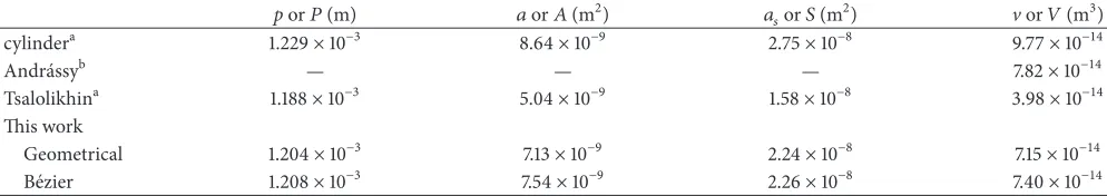
Plotting 𝑦(𝑡) against 𝑥(𝑡) (30) yields the B´ezier curve in the upper half of Figure 1(a). Since the nematode is symmetrical the lower boundary is just−𝑦(𝑡) against𝑥(𝑡), which is also shown in Figure 1(a). At least two features of the form defined by (30) are inappropriate: at the anterior end the B´ezier curve forms a pair of loops and at the posterior end

𝑑𝑦/𝑑𝑥approaches zero. The former is a common feature of polynomial interpolation through more than a small number of points [32]. The latter is overcome by fitting a B´ezier curve clockwise through the coordinates on both sides of the nematode (Figure 1(b)). This 13-coordinate extended representation is reasonable at the posterior, but the Runge effect is amplified at the anterior. However, it is clear from Figure 1(b) that the lower surface is better described than the upper surface. In fact all except the anterior supplementary

coordinate are described well by the lower curve. This observation and the symmetry of the nematode prompted the use of that part of the curve from the anterior supplementary coordinate (1, 0) to the first of Cobb’s coordinates (0.001,

−0.004) to model both the upper and lower boundaries of the nematode (Figure 1(c)). The dotted line underneath Figure 1(c) indicates the portion of the B´ezier curve that was used to generate the upper side of the nematode by reflection around the horizontal axis. The remainder of the anterior boundary was completed by linear interpolation from the anterior supplementary coordinate(0, 0)to (0.001, 0.004) and to (0.001,−0.004).

5. Comparison of Estimates of

𝑝

,

𝑎

,

𝑎

, and

V

The geometric and B´ezier representations ofA. antarcticus

described here are bounded by the cylindrical model and they enclose Tsalolikhin’s model (2) completely (Figure 2). As (2) can be rewritten as

𝑉_𝑇= 1₂𝜋𝐿₃ [(𝑑2+ 𝑑𝐷 + 𝐷₄ 2) + 𝐷₄2] , (31)

it is apparent that (2) represents an average of the volumes of a cone (diameter𝐷and length𝐿) and a conical frustum (length

0.01L

0.1L

0.01L

0.1L

(0.001, −0.004) (1, 0)

0.01L

0.1L

(a)

(b)

(c)

Figure 1: The development of the unweighted B´ezier representation ofAplectus antarcticus.The morphometric data of Cobb [21] (e) and two supplementary coordinates (I, (0, 0) and (1, 0)) are shown. The 7-coordinate version of the unweighted B´ezier representation (27)– (30) is the solid line in (a), which is reflected along the horizontal axis to give the dashed line in (a). The extended 13-coordinate B´ezier representation in (b) is explained in the text, as is the edited extended representation (c) that is derived from it. The dotted line in (c) represents the region from (0.001,−0.004) to (1, 0) that is reflected about the horizontal axis to form the upper boundary. Note that the vertical and horizontal dimensions differ in scale by a factor of 10 relative to the overall length of the nematode (𝐿= 0.6 mm).

is equivalent to (15) for𝑛 = 2, which might be the case for reports of the de Man indices (3).

The geometrical model represents the convex hull ofC (Figure 2), which necessarily provides a minimum estimate of𝑝 and𝑎. The overestimation inherent in the cylindrical estimate and the underestimation arising from Tsalolikhin’s model (2) are clear (Figure 2). To quantify this, the coordi-nates forA. antarcticus(28) were used to calculate𝑝,𝑎,𝑎_𝑠, and

V(or the corresponding values from the B´ezier representation (24)) (Table 1). As would be expected from Figure 2, the B´ezier and geometrical representations yield estimates that are similar and lie between those of the cylindrical and Tsalolikhin’s (2) models. Arbitrarily taking the geometrical representation as a reference, the cylindrical approach yields a volume 36% larger and (2) yields a value that is 44% smaller (Table 1). Even the value obtained from Andr´assy’s equation is 9% larger than the geometrical estimate, whereas the B´ezier estimate is only 3.5% larger (Table 1).

0.01L

0.1L

Figure 2: Comparison of the boundaries on which the estimates in Table 1 are based. The B´ezier (—) and geometric (-⋅-⋅-⋅-) representations are those we describe. The Tsalolikhin (- - - -) and cylindrical (. . . .) approximations have been reported previously. The morphometric data forA. antarcticusreported by Cobb [21] (e) and two supplementary coordinates (I, (0, 0) and (1, 0)) are shown. The vertical and horizontal dimensions differ in scale by a factor of 10 relative to the overall length of the nematode (L= 0.6 mm).

In the case ofA. antarcticusthe error in𝑉_𝑇arising just from the assumption that the point of greatest diameter is at

𝐿/2may be small. Nevertheless, it is instructive to consider a variant of (2) in which the weighting (𝜆) between the conical posterior and an anterior conical frustum can be varied. To do this we write (2) as

𝑉_𝑇(𝜆) = 𝜋𝐿 3 [𝜆 (

𝑑2_{+ 𝑑𝐷 + 𝐷}2

4 ) + (1 − 𝜆)

𝐷2

4 ]

= 𝜋𝐿₃ [𝜆 (𝑑2+ 𝑑𝐷₄ ) +𝐷₄2] ,

(32)

and the error arising from the midlength assumption is

𝜀_𝑇= 𝑉𝑇− 𝑉𝑇(𝜆)

𝑉_𝑇(𝜆) =

1 2

1 − 2𝜆

𝜆 + 𝐷2_{/ (𝑑}2_{+ 𝑑𝐷)}. (33) Applying (33) to the values forA. antarcticus, in which the widest point is located at 0.51Lrather than 0.5L, yields𝜀_𝑇=

−0.0036, so volume is only slightly underestimated, but Cobb [21] reports data for other species for which𝜆is larger. For example, forMonhystera polaris𝑑= 1.5,𝐷= 3.4, and𝜆= 0.64, so𝜀_𝑇=−0.063 which would be a significant underestimate for some purposes, even without any consideration of the other coordinates Cobb [21] reports.

6. Conclusion

Competing Interests

The authors declare that they have no competing interests.

References

[1] N. Muhamad, L. R. Walker, K. C. Pedley, D. C. Simcock, and S. Brown, “The initial kinetics of NH₃/NH₄+ efflux from L₃Teladorsagia circumcincta,”Parasitology International, vol. 61, no. 3, pp. 487–492, 2012.

[2] N. Muhamad, D. C. Simcock, K. C. Pedley, H. V. Simpson, and S. Brown, “The kinetic properties of the glutamate dehy-drogenase ofTeladorsagia circumcinctaand their significance for the lifestyle of the parasite,”Comparative Biochemistry and Physiology B: Biochemistry and Molecular Biology, vol. 159, no. 2, pp. 71–77, 2011.

[3] S. M. Sims, L. T. Magas, C. L. Barsuhn, N. F. H. Ho, T. G. Geary, and D. P. Thompson, “Mechanisms of microenvironmental pH regulation in the cuticle ofAscaris suum,”Molecular and Biochemical Parasitology, vol. 53, no. 1-2, pp. 135–148, 1992. [4] D. C. Simcock, S. Brown, J. D. Neale, S. M. C. Przemeck, and

H. V. Simpson, “L₃and adultOstertagia(Teladorsagia) circum-cinctaexhibit cyanide sensitive oxygen uptake,”Experimental Parasitology, vol. 112, no. 1, 7 pages, 2006.

[5] C. M. Stoscheck, “Quantitation of protein,”Methods in Enzy-mology, vol. 182, pp. 50–68, 1990.

[6] S. M. Sims, N. F. H. Ho, T. G. Geary et al., “Influence of organic acid excretion on cuticle pH and drug absorption by

Haemonchus contortus,”International Journal for Parasitology, vol. 26, no. 1, pp. 25–35, 1996.

[7] B. E. Hopper and E. J. Cairns,Taxonomic Keys to Plant, Soil and Aquatic Nematodes, Alabama Polytechnic Institute, Auburn, Ala, USA, 1959.

[8] L. W. McMurtry, M. J. Donaghy, A. Vlassoff, and P. G. C. Douch, “Distinguishing morphological features of the third larval stage of ovineTrichostrongylusspp.,”Veterinary Parasitology, vol. 90, no. 1-2, pp. 73–81, 2000.

[9] J. A. van Wyk, J. Cabaret, and L. M. Michael, “Morphological identification of nematode larvae of small ruminants and cattle simplified,”Veterinary Parasitology, vol. 119, no. 4, pp. 277–306, 2004.

[10] C. Hong and B. J. Timms, “Host-dependent variation in the morphology of femaleOstertagia circumcincta (Stadelmann, 1894) Ransom, 1907, a nematode parasite of sheep,”Systematic Parasitology, vol. 13, no. 2, pp. 121–124, 1989.

[11] G. Dikmans and J. S. Andrews, “A comparative morphological study of the infective larvae of the common nematodes parasitic in the alimentary tract of sheep,”Transactions of the American Microscopical Society, vol. 52, no. 1, pp. 1–25, 1933.

[12] K. B. Nguyen and G. C. Smart Jr., “Morphometrics of infective juveniles ofSteinernemaspp. andHeterorhabditis bacteriophora

(Nemata: Rhabditida),”Journal of Nematology, vol. 27, pp. 206– 212, 1995.

[13] L. Qiu and R. Bedding, “A rapid method for the estimation of mean dry weight and lipid content of the infective juveniles of entomopathogenic nematodes using image analysis,” Nematol-ogy, vol. 1, no. 6, pp. 655–660, 1999.

[14] G. J. Rau and G. Fassuliotis, “Equal-frequency tolerance ellipses for population studies ofBelonolaimus longicaudatus,”Journal of Nematology, vol. 2, no. 1, pp. 84–92, 1970.

[15] I. Andr´assy, “Die rauminhalts- und gewichtsbestimmung der fadenw¨urmer (Nematoden),”Acta Zoologica Academiae Scien-tiarum Hungaricae, vol. 2, pp. 1–15, 1956.

[16] O. Holovachov, Morphology and Systematics of the Order Plectida Malakhov, 1982 (Nematoda), Wageningen Universiteit, Wageningen, Netherlands, 2006.

[17] J. G. de Man, “Onderzoekingen over vrij in de aarde lev-ende nematoden,” Tijdschrift der Nederlandsche Dierkundige Vereeninging, vol. 2, pp. 78–196, 1876.

[18] J. G. de Man, “Die einheimischen, frei in der reinen Erde und im s¨ussen Wasser lebenden Nematoden,”Tijdschrift der Nederlandsche Dierkundige Vereeninging, vol. 5, pp. 1–104, 1881. [19] N. A. Cobb,A Nematode Formula, New South Wales

Depart-ment of Agriculture, Sydney, Australia, 1890.

[20] H. J. Van Cleave, “Expanding horizons in the recognition of a phylum,”The Journal of Parasitology, vol. 34, no. 1, pp. 1–20, 1948.

[21] N. A. Cobb, Antarctic Marine Free-living Nematodes of the Shakleton Expedition. Contributions to a Science of Nematology I, Williams and Wilkins, Baltimore, Md, USA, 1914.

[22] C. G. Goodchild and G. H. Irwin, “Occurrence of nematodes

Rhabditis anomala and R. pellio in oligochaetes Lumbricus rubellusandL. terrestris,”Transactions of the American Micro-scopical Society, vol. 90, no. 2, pp. 231–237, 1971.

[23] L. K. Eveland, T. Fujino, and B. Fried, “Scanning electron micro-scopical observations ofPellioditis pellio(Nematoda: Secernen-tia),”Transactions of the American Microscopical Society, vol. 109, no. 1, pp. 85–90, 1990.

[24] P. Jensen, “Nematodes from the brackish waters of the southern archipelago of Finland. Benthic species,” Annales Zoologici Fennici, vol. 16, pp. 151–168, 1979.

[25] M. Escuer, A. Palomo, and A. Bello, “The genusOgmaSouthern, 1914 (Nematoda: Criconematidae) in the Iberian Peninsula,”

Nematologica Mediterranea, vol. 18, no. 1, pp. 9–13, 1990. [26] A. C. Stewart and W. L. Nicholas, “New species of Xylidae

(Nematoda: Monhysterida) from Australian ocean beaches,”

Invertebrate Taxonomy, vol. 8, no. 1, pp. 91–115, 1994.

[27] G. Fonseca, W. Decraemer, and A. Vanreusel, “Taxonomy and species distribution of the genusManganonemaBussau, 1993 (Nematoda: Monhysterida),”Cahiers de Biologie Marine, vol. 47, no. 2, pp. 189–203, 2006.

[28] S. B. Fracker, “Variation in Oxyurias: its bearing on the value of a nematode formula,”Journal of Parasitology, vol. 1, no. 1, pp. 22–30, 1914.

[29] A. F. Robinson, “Comparison of five methods for measuring nematode volume,”Journal of Nematology, vol. 16, pp. 343–347, 1984.

[30] H. Engels, “A least squares method for estimation of Bezier curves and surfaces and its applicability to multivariate anal-ysis,”Mathematical Biosciences, vol. 79, no. 2, pp. 155–170, 1986. [31] T. M. Apostol,Calculus, vol. 1, John Wiley & Sons, New York,

NY, USA, 2nd edition, 1967.

[32] C. Runge, “ ¨Uber empirische funkionen und die interpolation zwischen ¨aquidistanten ordinaten,”Zeitschrift f¨ur Mathematik und Physik, vol. 46, pp. 224–243, 1901.

[33] H. J. Atkinson, P. E. Urwin, M. C. Clarke, and M. J. McPher-son, “Image analysis of the growth ofGlobodera pallidaand

[34] S. Das, W. M. L. Wesemael, and R. N. Perry, “Effect of temperature and time on the survival and energy reserves of juveniles ofMeloidogyne spp.,”Agricultural Science Research Journal, vol. 1, pp. 102–112, 2011.

[35] G. D. Tsibidis and N. Tavernarakis, “Nemo: a computational tool for analyzing nematode locomotion,”BMC Neuroscience, vol. 8, article 86, 2007.