University of Southern Queensland
Faculty of Engineering and Surveying
The Effects of Control Point Shape and Distribution in the Creation of
a Numeric Cadastral Data Base
A dissertation submitted by
David Roberts
in fulfilment of the requirements of
ENG4111 and 4112 Research Project
towards the degree of
Bachelor of Spatial Science (Honours) (Surveying)
I
ABSTRACT
For centuries information describing a parcel of land has been presented in the form of a hard copy
parchment or document. The information displayed on the face of such a document has traditionally
shown a direction and a distance along each line of each parcel. Since the advancement of angle and
distance reading instruments the accuracy of such plans has improved substantially. In saying this
surveyors dealing with older plans must determine, based on a hierarchy of evidence, how to deal
with the inconsistences between what is shown on the cadastral survey plan and what is actually
marked on the ground.
Recent advancements in processing power and surveying instrument capabilities have led to the
creation of what is known as a Numeric Cadastral Data Base (NCDB). Most states in Australia
currently utilize what is known as a Digital Cadastral Data Base (DCDB), which has limitations due
to the way it was originally created. A NCDB however is created by entering the cadastral/boundary
information from the original survey plan into a software package and then adjusting the network in
conjunction with the physical survey marks on the ground. The result is a survey accurate data base
which has the potential to be used as a means of better defining parcel boundaries.
This dissertation will investigate the processes involved in the creation of a NCDB and the effects of
control point selection within the cadastral adjustment. The results will show that the closest
representation to the boundaries actual position is achieved from the adjustment by using all of the
original survey marks. It was found that as control is added to the adjustment the mean difference
between the actual boundary corners and the adjusted corners became less over a test area of 49
parcels consisting of 147 corners. The research is supported by the Northern Territory Department of
Lands, Planning and the Environment (DLPE) and will contribute to the developing NCDB of the
II
University of Southern Queensland
Faculty of Health, Engineering and Sciences
ENG4111 & ENG4112 Research Project
Limitations of Use
The Council of the University of Southern Queensland, its Faculty of Health, Engineering and
Sciences, and the staff of the University of Southern Queensland, do not accept any responsibility for
the truth, accuracy or completeness of material contained within or associated with this dissertation.
Persons using all or any part of this material do so at their own risk, and not at the risk of the Council
of the University of Southern Queensland, its Faculty of Health, Engineering and Sciences or the staff
of the University of Southern Queensland.
This dissertation reports an educational exercise and has no purpose or validity beyond this exercise.
The sole purpose of the course pair entitled “Research Project” is to contribute to the overall
education within the student’s chosen degree program. This document, the associated hardware,
software, drawings, and any other material set out in the associated appendices should not be used for
III
Certification
I certify that the ideas, designs and experimental work, results, analyses and conclusions set out in this
dissertation are entirely my own effort, except where otherwise indicated and acknowledged.
I further certify that the work is original and has not been previously submitted for assessment in any
other course or institution, except where specifically stated.
David Roberts
IV
Acknowledgements
This research was carried out in conjunction with the Department of Lands Planning and the
Environment under the guidance of Licensed Surveyors Roland Maddocks and Paul Montefiore. I
extend my sincere appreciation to them both.
Appreciation is also due to Dr Glenn Campbell from the University of Southern Queensland for his
guidance and to Dr Mike Elfick from GeoData Australia for his willingness to answer questions
throughout the term of the project.
Lastly, many thanks are due to my employer Brian Blakeman for his flexibility throughout the year
V
TABLE OF CONTENTS
Contents
Page
ABSTRACT
I
Limitations of Use
II
Certification
III
Acknowledgements
IV
LIST OF FIGURES
VII
CHAPTER 1 -
INTRODUCTION
1
1.1 The Problem
1
1.2 Project Aims, (To investigate the effects of control point shape and distribution in the creation
of a NCDB)
2
1.3
Expected Outcomes and Benefits
3
CHAPTER 2 - LITERATURE REVIEW
4
2.1 Gathering of Information
4
2.1.1 The use of a NCDB in defining boundaries
4
2.1.2
Current Projects/Legislation
5
2.1.3 General Characteristics of a NCDB
6
2.1.4 Geodata, GeoCadastre and GeoSurvey
7
2.1.5
The Adjustment Process and Control Points
8
2.1.6 Previous NCDB Test Procedures
9
2.2 Review of Information
9
CHAPTER 3 - METHODOLOGY
11
3.1 Introduction
11
3.2 NCDB Creation
12
3.2.1 Original Survey Plan and Digital Data Acquisition (The Cadastral Fabric)
12
3.2.2 Field Reconnaissance and Field Work Planning
13
3.2.3
Coordinated Reference Mark (CRM) Placement
14
3.2.4 Conventional Field Traverse
15
3.2.5 GNSS Survey
16
3.2.6 NEWGAN Adjustment
16
VI
CHAPTER 4 - RESULTS
30
4.1 Introduction
30
4.2 Easting and Northing Boundary Corner Comparison
30
4.3 Distance Comparison
32
4.4 Distance Comparison Histograms and Normal Distribution
34
4.5 Manual Reinstatement vs Cadastral Adjustment Distance Vector Plots
35
4.6 Manual Reinstatement vs Cadastral Adjustment Mean Prediction
40
4.7 Control Density Test
41
CHAPTER 5 - DISCUSSION
42
5.1 Introduction
42
5.2 Easting and Northing Boundary Corner Comparison
42
5.3 Distance Comparison
43
5.4 Distance Comparison Histograms and Normal Distribution
45
5.5 Manual Reinstatement vs Cadastral Adjustment Distance Vector Plots
46
5.6 Manual Reinstatement vs Cadastral Adjustment Mean Findings
47
5.7 Summary
48
CHAPTER 6 - IMPLICATIONS AND CONCLUSIONS
49
6.1 Introduction
49
6.2 Implications
49
6.2.1 Points Inside and Outside the Control Configuration
49
6.2.2 Skewed Adjustments
50
6.2.3 Fully Constrained, at What Cost?
50
6.3 Further Research and Recommendations
52
6.4 Conclusions
55
LIST OF REFERENCES
56
APPENDICIES
59
VII
LIST OF FIGURES
Figure 1: Research Area
11
Figure 2 : ACS File provided to the Student by the DLPE
12
Figure 3 : Summary of Survey Marks within the Subject Area
13
Figure 4 : Feno Mark Installation Diagram
15
Figure 5 : NEWGAN Adjustment Summary
17
Figure 6 : Outputted CRMs and ORMs from NEWGAN Adjustment
18
Figure 7 : Parcel Properties
19
Figure 8 : Lines Tab
19
Figure 9 : Original Cadastral Plan Information
20
Figure 10 : Add Control 1
21
Figure 11 : Add Control 2
21
Figure 12 : Adjust Job
23
Figure 13 : Manually Reinstated Lots
24
Figure 14 : Convergence Calculated by Surveying Software
25
Figure 15 : Field Survey vs Original Survey
26
Figure 16 : Regular Quadrilateral 1
27
Figure 17 : Regular Quadrilateral 2
27
Figure 18 : Regular Triangle 1
27
Figure 19 : Regular Triangle 2
27
Figure 20 : Skewed East West Triangle 1
28
Figure 21 : Skewed East West Triangle 2
28
Figure 22 : Skewed North South Triangle 1
28
Figure 23 : Skewed North South Triangle 2
28
Figure 24 : Fully Constrained
29
Figure 25 : Regular Quadrilateral 1 Scatter Plot
30
Figure 26 : Regular Triangle 1 Scatter Plot
31
Figure 27 : Skewed East West Triangle 1 Scatter Plot
31
Figure 28 : Skewed North South Triangle 1 Scatter Plot
31
Figure 29 : Fully Constrained Scatter Plot
32
Figure 30 : Regular Quadrilateral 1 Column Graph
32
VIII
Figure 32 : Skewed East West Triangle 1 Column Graph
33
Figure 33 : Fully Constrained Column Graph
33
Figure 34 : Regular Quadrilateral 1 Histogram
34
Figure 35 : Regular Triangle 1 Histogram
34
Figure 36 : Skewed East West Triangle 1 Histogram
35
Figure 37 : Fully Constrained Histogram
35
Figure 38 : Regular Quadrilateral 1 Distance Difference Vector
36
Figure 39 : Regular Quadrilateral 2 Distance Difference Vector
36
Figure 40 : Regular Triangle 1 Distance Difference Vector
37
Figure 41 : Regular Triangle 2 Distance Difference Vector
37
Figure 42 : Skewed East West Triangle 1 Distance Difference Vector
38
Figure 43 : Skewed East West Triangle 2 Distance Difference Vector
38
Figure 44 : Skewed North South Triangle 1 Distance Difference Vector
39
Figure 45 : Skewed North South Triangle 2 Distance Difference Vector
39
Figure 46 : Fully Constrained Distance Difference Vector
40
Figure 47 : Manual Reinstatement vs Cadastral Adjustment Prediction
40
Figure 48 : Control Density Test
41
Figure 49 : Fully Constrained and 10 Point Traverse
52
1
CHAPTER 1
INTRODUCTION
1.1 The Problem
With the advancement in aerial photography came the potential to measure large areas of the earth’s
surface to a relatively high degree of accuracy. In conjunction with aerial photography cartographers
and surveyors were able to digitize old survey plans into a data base which was later to be known as a
Digital Cadastral Data Base (DCDB). The DCDB was however only as accurate as the digitizing
software and the base map at the time and could not be used as a sole source of boundary definition.
Due to the inaccuracies of the DCDB a new data base is being developed called the Numeric
Cadastral Data Base (NCDB). A NCDB is created by inputting the information from the original
cadastral plan into a software package and then adjusting the area in conjunction with the original
survey marks on the ground, ultimately to find the solution of best fit between the documentary and
physical evidence. The user is left with a mathematically consistent data base which shows the
individual parcels of an area relative to one another to a survey accurate standard.
Each point within the data base has its own coordinate value and the bearings and distances of each
line can also be reviewed. Because this data is already in a digital format to a high degree of accuracy
it has the potential to be loaded straight onto a total station or a global navigation satellite system
(GNSS) for the purpose of marking a parcel boundary.
Queensland is working on a NCDB through a company called SDX (Spatial Data eXchange) and
2
throughout the world in countries such as the USA, South Africa and the Philippines (Elfick,
Mclennan & Somers, unpub).
The Northern Territory is almost at a point where every parcel has been coordinated into a local
NCDB. This has mainly been done by the Northern Territory Government, Department of Lands
Planning and the Environment (DLPE), in conjunction with surveyors from private companies.
Because areas still need to be incorporated into the NCDB the potential for undergraduates to
contribute to the work done by the DLPE presents itself. The student has been assigned an urban area
in the western suburbs of the town of Alice Springs consisting of 280 parcels for research purposes.
1.2 Project Aims, (To investigate the effects of control point shape and
distribution in the creation of a NCDB)
Although NCDB’s are currently being developed in most states of Australia considerable research is
still required before any legal status can be assigned to such a data base. One area in particular is the
effect that control point shape and distribution has within the cadastral adjustment process. This
dissertation will investigate this area of research and aim to determine the effect of control point shape
and distribution in the creation of a NCDB. In order to investigate the project question the following
objectives have been created:
Gather the required information, relevant survey plans and/or digital data, to form the
cadastral fabric to be used within the NCDB.
Conduct the necessary field work by establishing a network of Coordinated Reference Marks
(CRMs) and traverse to original survey marks (ORMs) within the area.
Reduce all field data within the necessary software packages before making the cadastral
adjustment within the adjustment program GeoCadastre.
Using the cadastral fabric, generated from the original survey plans, combined with the data
3
The creation of NCDBs vary from state to state and it should be noted that this project will be
conducted in accordance with the methods put forward by the Northern Territory Department of
Lands, Planning and the Environment. Field work will be conducted in accordance with SP1
standards (Standard for the Australian Survey Control Network Special Publication 1, Version 2.1,
October 2014). In particular the Guidelines for Control Surveys by GNSS V2.1, Guidelines for
Conventional Traverse Surveys V2.1 and Guidelines for Installation and Documentation of Survey
Control Marks V2.1 (
Publications: Surveying Standards and Practices (SP1)
2016).
All data entry and field processing will be done under supervision of the Department of Lands,
Planning and the Environment to ensure quality as there is potential for this work to contribute to the
existing NCDB of Alice Springs. The area consists of 280 parcels and is made up of 33 survey plans
ranging from 1970 to 2014.
1.3
Expected Outcomes and Benefits
The project will provide the reader with specific information in regards to creating an NCDB and
make recommendations on the desired number and configuration of control points to be used during
the cadastral adjustment within the software package GeoCadastre.
The expected outcomes of the project include:
Identification of the process in developing a Numeric Cadastral Data Base using modern
surveying instruments and software packages.
Identify the effects of control point shape and distribution in the cadastral adjustment process
by comparing a range of adjustments using different control configurations to a manually
reinstated area.
Determine the expected accuracies of the Numeric Cadastral Data Base relative to the actual
4
CHAPTER 2
LITERATURE REVIEW
2.1 Gathering of Information
Further literature has been reviewed to develop the ideas towards the research project. The purpose of
the review was to gather relevant information in regards to:
The use of a NCDB in defining boundaries
Current Projects/Legislation
General characteristics of a NCDB
Geodata, GeoCadastre and GeoSurvey
The Adjustment Process and Control Points
Previous NCDB Test Procedures
2.1.1 The use of a NCDB in defining boundaries
A NCDB provides a survey accurate coordinate system which can provide a means of transition from
the current dimensional cadastral system to one based on fixed coordinates (Elfick, unpub, ACGMS).
Modern computer based Geographic Information Systems (GIS) and survey packages such as
Computer Aided Drafting (CAD) programs are position or coordinate orientated. Each point has an
easting, northing and height, in some cases, as well as different attributes such as description code
5
The survey instruments of today also utilise positional data in the form of co-ordinated values and are
able to locate a point on the earth’s surface to a much higher degree of accuracy then previous
methods. Because computer based geographical information systems are position orientated it can be
argued that there is a need for the cadastral system to be in a form compatible with all other
geographical based data sets (Elfick 1997).
In saying this careful considerations must be made if such a system is to be put in place. The
co-ordinate system currently used throughout Australia is the Geocentric Datum of Australia which is
based on the position, or epoch, of Australia in 1994. This forms the datum for grid coordinates Map
Grid of Australia 1994 (MGA94). Since this datum was established the continent of Australia has
moved under the MGA94 grid in a north easterly direction approximately seven centimetres a year
(ICSM 2015). This means that in the near future Australia will most likely adopt a more recent epoch
and in doing so will have to consider the effect on cadastral coordinate systems.
2.1.2
Current Projects/Legislation
Torrens Title is the system of land registration currently used in Australia and is historically based on
surveying land parcels and recording the ownership titles in the land registry. The Torrens system,
introduced in Australia between 1857 and 1875, is a system of title registration where the state
guarantees that the person shown on the title register is the registered proprietor (Dalrymple,
Williamson & Wallace, unpub).
This system proved to be much simpler than the previous method of deeds conveyancing which was
subject to problems caused by the nature of the chain of title. Under Torrens Title surveys of
individual parcel boundaries are carried out in relation to neighbouring parcels to a high mathematical
standard with support from the information shown on the original survey plans. This system has been
in place for 140 years and has proved to be effective. However, some issues do arise when conducting
6
South Australia has started generating an accurate NCDB and Tasmania awarded a tender to generate
and integrate a NCDB into their existing system (Sandy & Harper 2012). Queensland is also working
on a NCDB through a company called SDX (Spatial Data eXchange). Rather than waiting for new
subdivision data SDX will receive spatial information directly where it will then be managed in a
digital environment (Elfick, Mclennan & Somers, unpub). NSW has over 4 million parcels in a
well-managed registry and are currently looking at introducing electronic plan examination during the
registration process (Elfick, Mclennan & Somers, unpub).
Under section 46A of the
Northern Territory of Australia Licensed Surveyors Act
2013
the Surveyor
General may declare an area of land in the Territory to be a coordinated survey area. The act also
states that surveys within a coordinated survey area must be done in accordance with an approved
methodology to delimit land boundaries by geodetic coordinates. The Northern Territory is almost at a
point where every parcel has been coordinated into a local NCDB and in July 2014 three areas were
gazetted and became the first declared areas in Australia, (Sandy 2014). These areas are Gunbalanya,
Milingimbi and Gapuwiak and are remote communities in the Arnhem Land area east of Darwin.
2.1.3 General Characteristics of a NCDB
A NCDB should ideally be constructed directly from original survey plans by entering the data from
the face of the plan into the software package. In general the plans kept within the land titles record
system contain all the necessary information for surveyors to build an NCDB. If the data is adequate
for surveyors to re-establish boundaries, then it is adequate to build a numerical data set (Elfick 2001).
In saying this necessary field verification must be undertaken to ensure a healthy balance between the
adoption of dimensions shown on documents and the existing survey marks on the ground.
For practical reasons a group of between 100 to 300 parcels are worked on at a time
(Maddocks &
West, unpub)
. All the data for each area should be entered and adjusted to a local area and a number
of survey marks coordinated and used as absolute control. The adjustment is then re-run to compute
7
framework has been adequately adjusted the remaining surveys can be added to complete the data
base. Any isolated parcels can be measured with Global Positioning Systems (GPS) or gathered from
previous survey data and brought straight into the system
(Maddocks & West, unpub)
. The final
NCDB is a combination of a number of survey plans and subdivision data where all necessary
information is included in the system.
2.1.4 Geodata, GeoCadastre and GeoSurvey
Geodata Information Systems Pty. Ltd. (Geodata) is a company formed in 2007 to provide specialised
skills in survey and GIS cadastral database management. It is responsible for the creation of the
adjustment software “GeoCadastre” and the survey software “GeoSurvey” which will be used
throughout this project. This software has been developed over the last twenty years by the
recognised leaders from Geodata Michael Elfick and Michael Fletcher. The Environmental Systems
Research Institute (ESRI) has recently bought the rights to use the GeoCadastre software in its GIS
software packages confirming that the Geodata software is one of the most effective models in
cadastral parcel management systems (Smith 2012).
GeoCadastre is a Microsoft Windows based program specifically designed to adjust the survey parcel
networks by least squares methods. Geodata describes GeoCadastre as a record to fabric program
designed to build a parcel network from survey plans and survey data, ultimately the creation of a
NCDB. GeoSurvey, described as a Survey Data and Coordinate Geometry Tool by GeoData, utilises
the adjusted parcel network from GeoCadastre for practical surveying purposes. It allows the user to
view parcel information in geodetic coordinate systems, MGA94, and configure unit settings from
grid bearings to true bearings and grid distances to ground distances. GeoSurvey conversions include
ACS, Autocad, Trimble and LandXML as well as a range of other file types (Software Solutions:
8
2.1.5
The Adjustment Process and Control Points
The adjustment process is a weighted least squares adjustment, where weight is allocated depending
on the time of survey. This information is allocated to the parcel during the initial data input when the
date of the survey is assigned. Parcels with a higher accuracy level from recent plans (higher weight)
adjust less than those with a lower accuracy level from older plans (lower weight) (The Least Squares
Adjustment Process: About the least squares adjustment 2009). Having said this some cadastral
surveyors may argue that those marks closest in time to the original survey have the highest status and
weight.
The first step of the adjustment process determines the transformation parameters (rotation, scale and
translation) between the original coordinates of the control points and the corresponding coordinates
of their underlying parcel points. The control points used in the creation of the NCDB are the Original
Reference Marks, (ORMs), related to the original cadastral plan and should be permanent physical
features which can be adopted by future surveyors. It should be noted that the control point coordinate
values are held fixed in the least-squares adjustment and a minimum of two control points are
required to run the least-squares adjustment (The Least Squares Adjustment Process: About the least
squares adjustment 2009).
If the transformation residuals are within the specified limits, (based on the relationship between the
documentary and physical evidence), the parameters are applied to all the parcel corners to transform
them into the coordinates of the control system. The original bearing and distance of each line from
the initial survey plan input is compared with the bearings and distances in the transformed coordinate
system and any line that exceeds the set bearing and distance tolerance, (set by the user), is reported.
Once the coordinates have been transformed into the control system the adjustment engine varies the
coordinates and determines a best fit solution for all the points in the network (The Least Squares
9
2.1.6 Previous NCDB Test Procedures
After the cadastral data has been entered into the software package and the necessary adjustment
made, by least squares, a comparison can be conducted between the control co-ordinates and the
original cadastral values. An example can be shown within the town of Bachelor NT in a study
conducted by Maddocks. 16 cadastral plans were compiled consisting of 190 parcels and 35
co-ordinated points. Once the parcels had been joined four of the co-co-ordinated points were used as
control and the area adjusted. The remaining points were then used as a check to test the agreement
between the adjusted cadastre and the physical marks on the ground.
It was found that four control points with fixed values held the original parcel dimensions well with
the standard residuals on the test points being 19mm and the largest error 38mm
(Maddocks & West,
unpub)
. It was proven that the quality of the data largely depends on the age of the surveys and for
this reason considerations need to be made when comparing plan measurements to the geodetic
control. When assessing accuracy, it is also necessary to assess the quality of the instruments used at
the time of survey.
Steel chain and theodolite – by regulation needed to be good to 1:5,000 in country with slopes
not exceeding 4 degrees, however it could be as good as 1:10,000.
Invar Chain and theodolite – The expectation of work done with these instruments was
accuracies of better than 1:25,000.
EDM and theodolite – Expected to yield accuracies better than 1:30,000
(Maddocks & West, unpub)
2.2 Review of Information
A NCDB should be constructed directly from original survey plans by entering the data from the face
10
high enough standard to define property boundaries then they are suitable to be used for the creation
of a NCDB. Modern surveying software packages are position orientated as are the instruments of
today which are capable of defining a point on the earth’s surface to a much higher degree of accuracy
than ever before.
The control points used in the creation of the NCDB are the Original Survey Marks related to the
original cadastral plan and should be permanent physical features which can be adopted by future
surveyors. Previous studies have found that if a NCDB is created and adjusted correctly it can produce
results of a high degree of accuracy,
(Maddocks & West, unpub)
. It is important to keep in mind the
11
CHAPTER 3
METHODOLOGY
3.1 Introduction
The aim of this chapter is to precisely describe the method and materials required to create a NCDB.
It will also discuss the procedures used to test the effects of control point shape and distribution within
the cadastral adjustment. Firstly the procedures required to gather the necessary data for a NCDB will
be investigated and then an overview of the cadastral adjustment program GeoCadastre will be
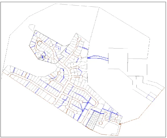
discussed. The area of interest allocated to the student by the DLPE within the Town of Alice Springs
is shown in the aerial image outlined in yellow below.
12
3.2 NCDB Creation
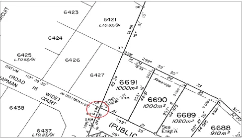
3.2.1 Original Survey Plan and Digital Data Acquisition (The Cadastral Fabric)
The subject area consists of 280 parcels and is made up of 33 survey plans ranging from 1970 to
2014. The information shown within these plans, (boundary dimensions and directions/bearings),
formed the basis of the cadastral fabric. The cadastral fabric is a continuous surface of connected
parcels and represents the original plan information. It is created within GeoCadastre by entering in
the bearing and distance for each line of every parcel from the cadastral plan data. This surface is
adjusted with the physical survey marks on the ground to form the NCDB. As the subject area was of
interest to the DLPE the initial data entry had already been completed.
This file, (the cadastral fabric), was in ACS format, (compatible with GeoCadastre), and represented
the original plan information. The file approximately fell on MGA94 Zone 53 as it had been
temporarily combined with the surrounding adjusted parcels in the local cadastre. All parcel
dimensions and bearings within the cadastral fabric represented original bearings and original ground
distances shown on the cadastral survey plans. In total the ACS file consisted of 898 corners 2,119
[image:21.595.159.437.510.739.2]bearings and 1,941 distances.
13
3.2.2 Field Reconnaissance and Field Work Planning
By using the ACS file provided by the DLPE the total number of original survey marks within the
subject area could be estimated. This was done by looking at each survey plan in chronological order
and plotting the ORMs position within the cadastral fabric. As the file was approximately coordinated
on MGA94 it could be loaded onto a Global Navigation Satellite System (GNSS) controller, and in
conjunction with a GNSS receiver used to search for the ORMs to be used in the creation of the
NCDB.
As the majority of ORMs within the area were drill holes located in the kerb of the road they were
easily identified and when located painted with a white circle to aid in future recovery. A note was
also made if the ORM was located, disturbed or gone. During this process a proposed position to
place the Coordinated Reference Marks (CRMs) was measured. These marks would later be used as
traverse stations to accurately measure the ORMs and will be discussed in more detail in the
following section.
Within the subject area 28 Brass Plugs were located, 10 nails, 76 drill holes and 9 spikes. 31 ORMs
were gone as they had been lost in driveways, footpaths or pram ramps and 89 ORMs were not
located as the back of the parcels were inaccessible and beyond the extent of the research project. This
would not affect the future analysis on the control selection as the area later selected for testing was
fully encompassed by ORMs. It was estimated that 45 CRMs would be required to traverse the ORMs
due to the irregular street network and undulating terrain of the subject area.
Figure 3 : Summary of Survey Marks within the Subject Area
Brass Plugs
Nails
Drill Holes
Spikes
Gone
Unlocated
14
3.2.3
Coordinated Reference Mark (CRM) Placement
In order to gather the required data for the creation of the NCDB a network of CRMs needed to be
established from which the ORMs could be measured. The placement of the CRMs throughout the
subject area was done in accordance with the ICSM Guideline for the Installation and Documentation
of survey Control Marks Special Publication 1 Version 2.1 and the Northern Territory of Australia
Survey Practice Directions – Surveys within Coordinated Survey Areas 2003 (NT). The ICSM
Guidelines state the survey control mark should be made of good quality, durable, corrosion resistant
materials and be placed where it is least likely to be disturbed, damaged or removed.
Under the Northern Territory Practice Directions the surveyor must ensure that the CRM is
constructed of a material that will resist destruction by fire, decay and termites. The CRM itself
should be permanently marked with a unique station identifier to ensure unambiguous identification
and a station identifier associated with the survey mark. The mark should be located in a position that
maximises the use of different measurement techniques and connection to future marks. This was
necessary to ensure that the CRMs could be measured directly using conventional traversing methods
as well as GNSS techniques.
In total 46 new CRMs were placed, 31 by the student and 15 by the DLPE. The majority of the marks
were placed roughly 0.3m from the back of the road kerb at street intersections and at the end of
cul-de-sac’s. These marks, Polyroc FENO Mark, were placed at intervisible locations from which the
ORMs could be measured. The FENO mark, developed in the 1970’s by the French company Faynot
consists of three components; a 610mm anchor or spike, a polyroc head and an aluminium insert.
The FENO mark is placed by first driving the anchor into the ground with the Polyroc Head between
the natural surface and the lip of the anchor. A driving tool is then placed in the anchor tube and
driven down to cause the extension of the three prongs which firmly lock the mark to the ground. The
aluminium insert which has the CRM number and centering hole punch is then inserted into the
15
Figure 4 : Feno Mark Installation Diagram
The aluminium insert was stamped with the unique CRM identifier which consisted of the survey plan
number S16064, allocated by the Surveyor General, followed by the point number, e.g. S16064002.
Part 5 of the Northern Territory of Australia Survey Practice Directions states that the surveyor must
ensure that the CRM is accompanied with a warning tag affixed to a witness mark or other substantial
structure. In the case of the research area a witness plate with recovery information, (magnetic bearing
and distance from the plate to the CRM), and CRM number was placed adjacent to the CRM in the
kerb of the road or footpath.
3.2.4 Conventional Field Traverse
The field traverse was conducted in accordance with the Guideline for Conventional Traverse Surveys
Special Publication
1. The student traversed CRMs 1 - 31 and the DLPE traversed the remaining 32 -
46. A Leica TCR1105 Total Station, (5 second angle measuring accuracy), was used to conduct the
field traverse to accurately measure the position of the ORMs in relation to the CRMs. Before the
commencement of field work the instrument was calibrated at the Morrie Hocking Baseline, Alice
Springs.
Tribrach’s with Optical Plummet and precision carriers, (GDF322 Tribrach with Optical Plummet and
Leica GZR3 Precision Carrier), and Leica GPR1 Circular Prism’s were used with Wooden Tripods,
(Leica GST20 Wooden Tripod), when measuring between traverse stations. Observations to ORMs
less then 30m away were taken using a low set Leica mini prism positioned low on the pole to ensure
16
tripod. This helped eliminate incorrect angle reading errors which are exaggerated as distance
increases, (20 seconds of arc is the equivalent to 10mm over 100m). This equipment satisfied a
Survey Uncertainty, SU, and Relative Uncertainty, RU, of less than 10mm (ICSM 2014).
The field traverse consisted of measuring face left and face right horizontal angles, vertical angles,
horizontal distances and slope distances between traverse stations (CRMs) and radiations to ORMs.
Naming of ORMs were with sequential alpha suffixes clockwise from north, e.g.
S16064023A, S16064023B, S16064023C etc for all marks radiated from CRM S16064023. T
he
mean of any angle did not exceed 10” over an observation greater than 50m. Instrument and target
heights were measured and temperature and pressure readings taken on a regular basis, or at
pronounced changes in conditions.
These readings were input into the atmospheric corrections within the Total Station in the field. This
was done to ensure that the correct ppm (parts per million) correction was applied to the measured
distances. This compensates for errors in the Electric Distance Measurement (EDM) due to
fluctuations in the speed of light caused by temperature and pressure through which light passes
through (Professional Surveyor Magazine
2004). These procedures satisfied a SU and RU of less than
10mm (ICSM 2014).
3.2.5 GNSS Survey
In conjunction with the conventional field traverse CRMs 1-46 were measured by the DLPE using
Static GNSS techniques. Four dual frequency geodetic receivers were used in each session and three
Continually Operating Reference Stations (CORS) were used to resolve the ambiguities. Further
redundancy was achieved by occupying the CRMs twice.
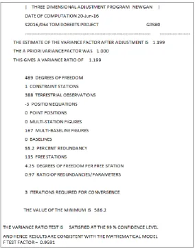
3.2.6 NEWGAN Adjustment
The three dimensional least squares adjustment program NEWGAN was used by the DLPE to
17
were input into the adjustment program as the required terrestrial information was not available for
CRMs 32-46.
In total 115 stations were input into NEWGAN, (3 CORS Stations, 31 CRMs and 81 ORMs). One
CORS station was assigned as constrained. Latitude, Longitude and Elevation gathered from the
GNSS survey were input for the CRMs and for the ORMs an approximate co-ordinate which was
extracted from the cadastral fabric.
The terrestrial directions and distances, (slope), were also input into the program. AHD elevations
were obtained for the CRMs by conventional levelling techniques from neighbouring bench marks
within the area by the DLPE. The following information extracted from the NEWGAN report further
[image:26.595.156.441.362.723.2]summarises the variables of the adjustment.
18
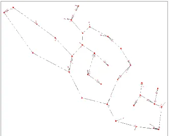
The results file from the NEWGAN adjustment produced MGA94 Zone 53 coordinates and AHD
levels for CRMs 1-31, (shown as squares), and 81 ORMs, (shown as crosses). These coordinates
[image:27.595.132.464.181.448.2]would later be used when testing the cadastral adjustment within GeoCadastre, (see appendix B).
Figure 6 : Outputted CRMs and ORMs from NEWGAN Adjustment
3.2.7 GeoCadastre Cadastral Adjustment
Ten adjustments were made in GeoCadastre using different control shapes resembling similar
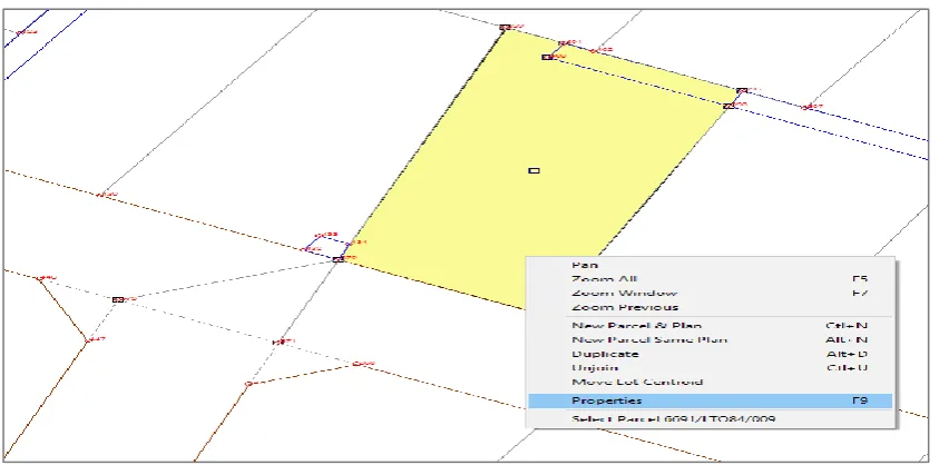
configurations commonly used by Surveyors. The first step within the adjustment is selecting points
within the cadastral fabric of GeoCadastre and assigning them as ‘control’. This is done by first
adding the ORM to the cadastral fabric. To add points to the cadastral fabric the properties of the
19
Figure 7 : Parcel Properties
Once the parcel properties has been selected the ORM can be added by entering the bearing and
distance from the selected parcel corner using the radiation information from the original survey plan.
This is done in the Lines Tab.
[image:28.595.78.560.405.735.2]20
Figure 9 : Original Cadastral Plan Information
The ‘From’ point can be selected from the existing points within the file, however the ‘Bearing’ and
‘Distance’ must be manually entered. The ‘To’ column is the point number given to the new point, if
an existing number is input a new number will automatically be assigned. The ‘Type’ is set to 995 for
a control point; this will hold the connection from the ORM to the boundary corner fixed in the
adjustment and will be represented by a red dashed line.
Once the ORM has been input into to the cadastral fabric it can then be added to the control list to be
used in the least squares adjustment. This is done by selecting the ‘Adjust’ tab and then ‘Control’. In
the Control function ‘Add’ is then selected and the ORM highlighted using the cursor or the point
21
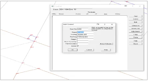
Figure 10 : Add Control 1
The coordinates of the control point displayed at this stage are the unadjusted coordinates from the
cadastral fabric, approximately MGA94 Zone 53 as previously discussed in 3.2.1. It is here that the
measured coordinates and height from the NEWGAN adjustment are input. The correct Name for the
control point should also be entered.
[image:30.595.74.549.500.741.2]22
When manually adding control points the association between the fabric point and the control point
can be immediately established, (E∆ 0.011m and N∆ .015m). Having the control point active will
assign the point as active once the ok box is selected. Active control points are used in the least
squares adjustment, inactive control points are excluded from the adjustment. This procedure is
repeated for each ORM until the desired number of control points has been reached. Within the
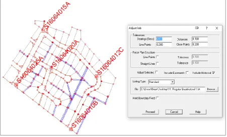
‘Control’ function ‘Adjustment’ is then selected which will open the ‘Adjust Job’ function. Within
the ‘Adjust Job’ the adjustment tolerances can be set which will report on the bearings, distances, line
points and close points which exceed the set tolerances between the difference of the adjusted line and
the original recorded line.
The adjustment settings can also be configured to force line points or straight lines. These options
were not selected for the testing of the adjustment. Parcels can be isolated and adjusted individually
by selecting the ‘Adjust Selected’ box and easements also included in the adjustment by selecting
‘Include Easements’. These two settings were also unselected during the testing of different control
configurations. The ‘Include Historical’ box was selected during the testing phase. As mentioned in
2.1.5 weight is allocated depending on the date of survey which is assigned to each parcel during the
creation of the cadastral fabric.
The ‘Listing Type’ can be configured to produce a more detailed report of the adjustment however as
the adjusted coordinates of the boundary corners were all that was required for future testing, the
standard setting was used. ‘Hold Boundary Fixed’ was not selected as the purpose of the adjustment
was to generate adjusted boundary corners from different ORM configurations. Once all settings have
23
Figure 12 : Adjust Job
The Adjustment will then run and if successful generate an adjustment summary. The report gives a
statistical summary on the number of points and lines in the adjustment and alerts if any tolerances
were exceeded. The maximum and average shift is reported between the original cadastral fabric and
the adjusted parcel corners. A results file is also produced which gives a summary of the effect of the
adjustment on each parcel and every line within the fabric.
A complete list of the final boundary coordinates is given in the results file. These were in the form of
MGA94 Zone 53 coordinates and were extracted from the results file after each adjustment was run.
These coordinates would be used for comparison and future testing of control configuration.
3.3 Preliminary Testing Considerations
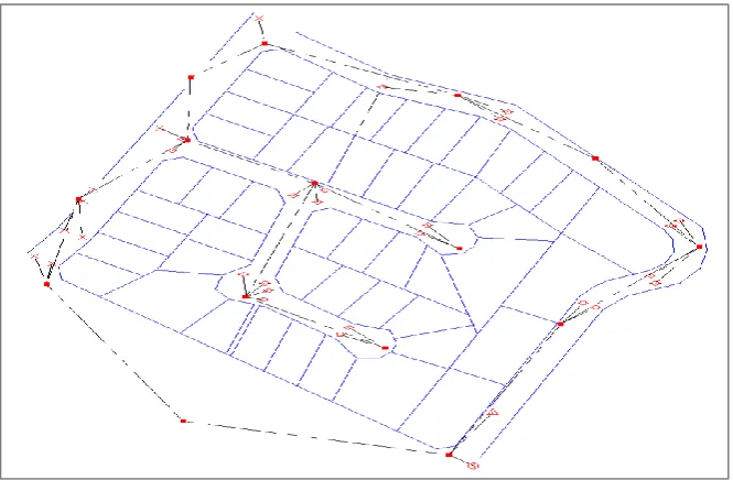
From the adjusted NEWGAN coordinates 15 CRMs were selected which encompassed an area
consisting of 48 parcels, 147 corners and 32 ORMs. The area was reinstated manually which formed a
24
NEWGAN coordinates were MGA94 the area was reinstated in a Universal Transverse Mercator
Projection, (UTM), Map Grid Australia 94 Zone 53. Reinstating the boundaries in MGA94 was
[image:33.595.132.465.157.375.2]necessary as the adjusted boundaries from GeoCadastre would also be in the form of grid coordinates.
Figure 13 - Manually Reinstated Lots
Liscad SEE, Surveying and Engineering Environment Version 12.0, was used to conduct the manual
reinstatement. Unit configurations were set to ground distances and bearings set to Azimuth/True
Bearings. The difference between MGA94 Grid Bearings and True Bearings, (Grid Convergence), in
the subject area was between - 27’ 40’’ and - 27’45”. For example at CRM S16064020A (Lat -23° 42’
5.86”, Long 133° 51’ 4.49”):
Tan Grid Convergence =
–Sin Lat point. Tan (Long point – Long CM)
Where CM is the Central Meridian (135° for zone 53)
Lat Point is the latitude of the point of interest
Long Point is the Longitude of the point of interest
(Department of Sustainability and Environment)
Tan Grid Convergence =
-Sin -23.7016277778. Tan(133.851247222 – 135)
25
=
-0.00806046094181
=
Arc Tan (-0.0080604694181)
=
-0.461820391419 (Decimal Degree’s)
=
- 27’ 43”
The same convergence is achieved when analysing the point within Liscad as seen in the figure
below.
Figure 14 : Convergence Calculated by Surveying Software
Cadastral survey plans within Alice Springs use grid bearings which are based on a local grid of the
town. The local grid was determined by measuring an azimuth from the centre of the town, at
ANZAC Fundamental to Mt. Everard, which became the datum of the grid. At this line the
observation was a true bearing however as surveys were taken further from the datum line the
bearings no longer resembled a true bearing. The subject area was roughly 3.2km west from the initial
point of the local grid. When comparisons made between the field data, with units configured to true
bearings, and the original survey plan data the convergence between the local grid and true bearings
was negligible. Some comparisons between the manual reinstatement and the original survey plan can
26
Figure 15 - Field Survey vs Original Survey
From the NEWGAN coordinates, with units configured to ground distances and the azimuth to true
bearings, the subject area was reinstated from the ORM’s using the local cadastral grid bearings and
distances from the original survey plans. Excess and shortage was distributed evenly throughout the
area so that no lot was favoured over another. No major disagreement was found between the original
survey plans and the measured field data. This became the base file which would be used to compare
the position of the boundary corners created after each adjustment within GeoCadastre.
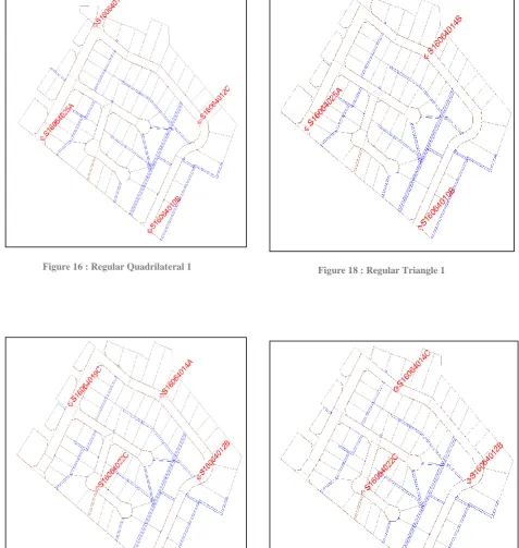
3.4 Test Cadastral Adjustment Configurations
Initially 9 cadastral adjustments were conducted in GeoCadastre using configurations commonly used
in surveying practices. The resulting 147 boundary corners from each adjustment would then be
compared to the corners from the manual reinstatement in 9 separate comparison files. The different
configurations included two Regular Quadrilateral, two Regular Triangle, two Skewed East West, two
Skewed North South and one Fully Constrained adjustment. It should be noted that the skewed
adjustments were included to deliberately resemble a poor adjustment and would not be normally
27
Figure 16 : Regular Quadrilateral 1
[image:36.595.68.546.131.635.2]Figure 17 : Regular Quadrilateral 2
Figure 18 : Regular Triangle 1
[image:36.595.72.552.403.674.2]28
[image:37.595.74.295.119.359.2]Figure 20 : Skewed East West Triangle 1
Figure 21 : Skewed East West Triangle 2
Figure 22 : Skewed North South Triangle 1
[image:37.595.73.543.414.665.2]29
30
CHAPTER 4
RESULTS
4.1 Introduction
If we compare the coordinates of the 147 corners generated from each adjustment to the manual
reinstatement the results can be expressed in a number of different ways. This chapter displays the
findings of the test adjustments through a series of graphs and visual plots. A detailed discussion of
the findings will be presented in Chapter 5. Four different graphical representations of the findings
have been included in this chapter to aid the reader in understanding the relationship between the
manual reinstatement and the GeoCadastre/Cadastral adjustment’s.
4.2 Easting and Northing Boundary Corner Comparison
These graphs compare the difference in easting and northing between the manual reinstatement and
the cadastral adjustment. The horizontal axis represents the boundary corner and the vertical axis
represents the difference in easting and northing between the two points.
Figure 25 : Regular Quadrilateral 1 Scatter Plot
-0.100
-0.080
-0.060
-0.040
-0.020
0.000
0.020
0.040
0.060
0.080
0.100
1
21
41
61
81
101
121
141
D
is
ta
n
c
e
(
m
)
Boundary Corner
Regular Quadrilateral 1 GeoCadastre vs Manual Reinstatement Coordinate
Comparison
∆ E
31
[image:40.595.73.525.282.487.2]Figure 26 : Regular Triangle 1 Scatter Plot
[image:40.595.70.531.540.741.2]Figure 27 : Skewed East West Triangle 1 Scatter Plot
Figure 28 : Skewed North South Triangle 1 Scatter Plot
-0.100
-0.080
-0.060
-0.040
-0.020
0.000
0.020
0.040
0.060
0.080
0.100
1
21
41
61
81
101
121
141
D
is
ta
n
c
e
(
m
)
Boundary Corner
Regular Triangle 1 GeoCadastre vs Manual Reinstatement Coordinate Comparison
∆ E
∆ N
-0.100
-0.080
-0.060
-0.040
-0.020
0.000
0.020
0.040
0.060
0.080
0.100
1
21
41
61
81
101
121
141
D
is
ta
n
c
e
(
m
)
Boundary Corner
Skewed East West Triangle 1 GeoCadastre vs Manual Reinstatement Coordinate
Comparison
∆ E
∆ N
-0.100
-0.080
-0.060
-0.040
-0.020
0.000
0.020
0.040
0.060
0.080
0.100
1
21
41
61
81
101
121
141
D
is
ta
n
c
e
(
m
)
Boundary Corner
Skewed North South Triangle 1 GeoCadastre vs Manual Reinstatement Coordinate
Comparison
∆ E
32
Figure 29 : Fully Constrained Scatter Plot
4.3 Distance Comparison
If the distances between the cadastral adjustment corner and the manual reinstatement corner are
compared the results can be expressed by a column graph. The horizontal axis represents the
boundary corner and the vertical axis the difference between the position of the GeoCadastre
boundary corner and the manually reinstated corner.
Figure 30 : Regular Quadrilateral 1 Column Graph
-0.100
-0.080
-0.060
-0.040
-0.020
0.000
0.020
0.040
0.060
0.080
0.100
1
21
41
61
81
101
121
141
Dis
ta
n
c
e
(m
)
Boundary Corner
Fully Constrained GeoCadastre vs Manual Reinstatement Coordinate Comparison
∆ E
∆ N
0
0.01
0.02
0.03
0.04
0.05
0.06
0.07
0.08
1
21
41
61
81
101
121
141
D
is
ta
n
c
e
(
m
)
Boundary Corner
33
Figure 31 : Regular Triangle 1 Column Graph
Figure 32 : Skewed East West Triangle 1 Column Graph
Figure 33 : Fully Constrained Column Graph
0
0.01
0.02
0.03
0.04
0.05
0.06
0.07
0.08
1
21
41
61
81
101
121
141
D
is
ta
n
c
e
(
m
)
Boundary Corner
Regular Triangle 1 GeoCadastre vs Manual Reinstatement Distance Comparison
(μ = 0.023m, σ = 0.016m)
0
0.01
0.02
0.03
0.04
0.05
0.06
0.07
0.08
1
21
41
61
81
101
121
141
D
is
ta
n
c
e
(
m
)
Boundary Corner
Skewed East West Triangle 1 GeoCadastre vs Manual Reinstatement Distance
Comparison
(μ = 0.029m, σ = 0.017m)
0
0.01
0.02
0.03
0.04
0.05
0.06
0.07
0.08
1
21
41
61
81
101
121
141
D
is
ta
n
c
e
(
m
)
Boundary Corner
34
4.4 Distance Comparison Histograms and Normal Distribution
These histograms represent the number of times a boundary corner generated from the cadastral
adjustment fell within a specified difference to the manual reinstatement. Using the distance
comparison means and standard deviations we can also create a normal distribution curve to analyse
the spread of the data and the probability of arriving at a value.
Figure 34 : Regular Quadrilateral 1 Histogram
Figure 35 : Regular Triangle 1 Histogram
0
0.01
0.02
0.03
0.04
0.05
0.06
0.07
0.08
0.09
0
10
20
30
40
50
60
70
80
90
0
10
20
30
40
50
60
70
80
90
Fr
e
q
u
e
n
c
y
Bin (mm)
Regular Quadrilateral 1 Histogram with Normal Curve
Frequency
Probalility E
0
0.01
0.02
0.03
0.04
0.05
0.06
0.07
0.08
0.09
0
10
20
30
40
50
60
70
80
90
0
10
20
30
40
50
60
70
80
90
Fr
e
q
u
e
n
c
y
Bin (mm)
Regular Triangle 1 Histogram with Normal Curve
Frequency
35
Figure 36 : Skewed East West Triangle 1 Histogram
Figure 37 : Fully Constrained Histogram
4.5 Manual Reinstatement vs Cadastral Adjustment Distance Vector Plots
The following vector plots have been generated to examine the direction and magnitude of the
difference between the manual reinstatement and the cadastral adjustment. The direction of the arrow
is from the manually reinstated corner to the outputted corner from the GeoCadastre adjustment. The
length of the line displays the difference in metres between the two points in conjunction with the
scale bar. The blue triangles represent the position of the control points used in the adjustment.
0
0.01
0.02
0.03
0.04
0.05
0.06
0.07
0.08
0.09
0
10
20
30
40
50
60
70
80
90
0
10
20
30
40
50
60
70
80
90
Fr
e
q
u
e
n
c
y
Bin (mm)
Skewed East West Triangle 1 Histogram with Normal Curve
Frequency
Probalility E
0
0.01
0.02
0.03
0.04
0.05
0.06
0.07
0.08
0.09
0
10
20
30
40
50
60
70
80
90
0
10
20
30
40
50
60
70
80
90
Fr
e
q
u
e
n
c
y
Bin (mm)
Fully Constrained Histogram with Normal Curve
Frequency
36
Figure 38 : Regular Quadrilateral 1 Distance Difference Vector
[image:45.595.130.468.431.728.2]37
Figure 40 : Regular Triangle 1 Distance Difference Vector
[image:46.595.126.472.431.718.2]38
Figure 42 : Skewed East West Triangle 1 Distance Difference Vector
[image:47.595.115.483.426.727.2]39
Figure 44 : Skewed North South Triangle 1 Distance Difference Vector
[image:48.595.109.489.421.725.2]40
Figure 46 : Fully Constrained Distance Difference Vector
4.6 Manual Reinstatement vs Cadastral Adjustment Mean Prediction
In order to analyse the effects of control point density, 6 additional adjustments were run removing
points from the fully constrained configuration by five at a time. It was predicted that as more points
are removed, the mean difference between the manual reinstatement and the cadastral adjustment
[image:49.595.112.484.70.321.2]would become greater.
Figure 47 : Manual Reinstatement vs Cadastral Adjustment Prediction
0.000
0.005
0.010
0.015
0.020
0.025
0.030
0.035
5
10
15
20
25
30
P
o
int
t
o
P
o
int
D
if
fe
re
n
c
e
M
e
a
n
(
m
)
No. of Control Points
41
4.7 Control Density Test
This graph presents the findings after having run the adjustments mentioned in 4.6 and shows us that
as control is extracted from the adjustment the mean difference between the manual reinstatement and
[image:50.595.69.538.206.432.2]the cadastral adjustment becomes greater.
Figure 48 : Control Density Test
0.000
0.005
0.010
0.015
0.020
0.025
0
5
10
15
20
25
30
M
e
a
n
D
if
fe
re
n
c
e
(
m
)
No. of Control Points
42
CHAPTER 5
DISCUSSION
5.1 Introduction
The results obtained in Chapter 4 revealed that the configuration and density of control within the
cadastral adjustment has a direct effect on the final position of the boundary corner. This chapter will
discuss in detail the results obtained in Chapter 4 and will then lead into a deliberation on the
implications of the results in the following chapter.
5.2 Easting and Northing Boundary Corner Comparison
When comparing the coordinates of the manual reinstatement to the cadastral adjustment a scatter plot
can be generated to analyse the relationship between the two data sets. If the difference between the
manual reinstatement and the cadastral adjustment is significant then we would expect the scatter plot
to vary from the middle of the graph at the zero difference line. If the two data sets resemble similar
coordinates over the 147 corners then we would expect that the scatter plot be clustered around the
centre of the graph.
When analysing the regular quadrilateral configuration we can see that the easting of the corners
generated from the cadastral adjustment resembled the easting of the manual reinstatement slightly
better than that of the northing. We can also see from the graph that the largest difference in the
easting was 38mm and the largest difference in the northing 53mm. The standard deviation between
the regular quadrilateral and the manual reinstatement was 11mm in the easting and 26mm in the
43
If we look at the regular triangle configuration it can be seen that both the difference in easting and
northing fluctuate around the centre of the graph. Using this configuration gave a largest difference in
easting of 71mm and a largest difference in northing of 48mm. The standard deviation of the data set
was 21mm in the easting and 18mm in the northing.
Interesting observations can be made when analysing the skewed east west triangle and skewed north
south triangle scatter plot. It can be seen that if the control is skewed in an east west running line then
the effect on the northing will be greater than the effect on the easting. The same can be said when the
control is running in a north south direction. If the control is skewed in a north south running line then
the effect of the easting will be greater than that of the northing. This is supported by the high and low
differences between the data sets.
With the skewed east west configuration the largest difference in the easting was 32mm and the
largest difference in the northing was 77mm. With the skewed north south triangle the largest
difference in easting was 84mm and the largest difference in the northing was 57mm. It was found
that the standard deviation between the manual reinstatement and the skewed east west triangle was
13mm in the easting and slightly more in the northing with 31mm. The skewed north south triangle
had a standard deviation of 29mm in the easting and slightly less in the northing of 19mm.
When analysing the fully constrained scatter plot it can be seen that the data is much more clustered
around the centre of the graph giving a better representation of the manual reinstatement. The largest
difference in easting was 15mm and the largest difference in northing was 34mm. The standard
deviation in the easting and northing was therefore much lower than all other configurations with a
5mm standard deviation in easting and 8mm standard deviation in northing.
5.3 Distance Comparison
If the distances between the cadastral adjustment corner and the manual reinstatement corner are
44
between the two data sets a mean difference can be calculated as all distances are positive. This could
not be done when analysing the difference in easting and northing as values can be negative when
comparing coordinates. If the data is represented by differences close to zero then the adjustment has
closely resembled the manual reinstatement.
The regular quadrilateral column graph shows us that the difference between the two data sets
fluctuated over the 147 corners. At points around corners 21, 61, 81 and 121 the difference between
the cadastral adjustment and the manual reinstatement was within 10mm however the difference often
reached 50mm over the rest of the graph. The mean difference generated from the regular
quadrilateral was 25mm with a standard deviation of 15mm when comparing the distance vector.
The regular triangle generated similar results when comparing the difference in distance between the
two data sets over the 147 corners. Again at points around corners 21, 61, 81,100 and 141 the