Preventive Medicine
&
Public Health
Preventive Medicine
&
Public Health
J Prev Med Public Health 2017;50:311-319 • https://doi.org/10.3961/jpmph.17.040Hazardous Alcohol Use in 2 Countries: A Comparison
Between Alberta, Canada and Queensland, Australia
Diana C. Sanchez-Ramirez1, Richard Franklin2, Donald Voaklander1,21Injury Prevention Centre, School of Public Health, University of Alberta, Edmonton, AB, Canada; 2World Safety Organization, Collaborative Centre
for Injury Control and Safety Promotion, College of Public Health, Medical and Veterinary Sciences, James Cook University, Townsville, OLD. Australia
Original Article
Objectives: This article aimed to compare alcohol consumption between the populations of Queensland in Australia and Alberta in Canada. Furthermore, the associations between greater alcohol consumption and socio-demographic characteristics were explored in each population.
Methods: Data from 2500 participants of the 2013 Alberta Survey and the 2013 Queensland Social Survey were analyzed. Regression analyses were used to explore the associations between alcohol risk and socio-demographic characteristics.
Results: A higher rate of hazardous alcohol use was found in Queenslanders than in Albertans. In both Albertans and Queenslanders, hazardous alcohol use was associated with being between 18 and 24 years of age. Higher income, having no religion, living alone, and being born in Canada were also associated with alcohol risk in Albertans; while in Queenslanders, hazardous alcohol use was also associated with common-law marital status. In addition, hazardous alcohol use was lower among respondents with a non-Catholic or Protestant religious affiliation.
Conclusions: Younger age was associated with greater hazardous alcohol use in both populations. In addition, different socio-demo-graphic factors were associated with hazardous alcohol use in each of the populations studied. Our results allowed us to identify the socio-demographic profiles associated with hazardous alcohol use in Alberta and Queensland. These profiles constitute valuable sources of information for local health authorities and policymakers when designing suitable preventive strategies targeting hazard-ous alcohol use. Overall, the present study highlights the importance of analyzing the socio-demographic factors associated with al-cohol consumption in population-specific contexts.
Key words: Alcohol drinking, Risk factors, Alberta, Queensland
Received: March 14, 2017 Accepted: July 14, 2017
Corresponding author: Richard Franklin, PhD
1 James Cook Drive, Townsville, QLD 4811, Australia Tel: +61-7-5781-5939
E-mail: richard.franklin@jcu.edu.au
This is an Open Access article distributed under the terms of the Creative Commons Attribution Non-Commercial License (http://creativecommons.org/licenses/by-nc/4.0/) which permits unrestricted non-commercial use, distribution, and repro-duction in any medium, provided the original work is properly cited.
INTRODUCTION
Alcohol imposes a significant economic and social burden worldwide. It is a causal factor of many diseases, as well as a
pISSN 1975-8375 eISSN 2233-4521
precursor to injury and violence [1]. As the harmful effects of alcohol are not constrained to a given country, studies com-paring the use of alcohol between countries have been under-taken [2,3]. However, such studies have mostly described the size of the problem, but have not further explored the socio-demographic factors associated with it. Furthermore, the com-parison of alcohol consumption across countries can be a use-ful mechanism to identify context-specific characteristics that may help tailor alcohol policies in specific cultural, political, and economic settings.
based on the Westminster system of government and have 3 tiers of government (local, state, and national). In addition, both countries have implemented approaches controlling the physical availability and the affordability of alcohol [4,5]. At the regional level, the province of Alberta in Canada and the state of Queensland in Australia have similar socioeconomic characteristics (i.e., a population of around 4 million [6,7], an annual gross domestic product close to 290 million (local cur-rency), as well as both agriculture-based and resource-based economies), which make the comparative study of alcohol consumption between them pertinent.
Size of the Problem and Context
According to the Organization of Economic Cooperation and Development (OECD), an estimated 8 liters of alcohol per capita were consumed in Canada in 2012 [8]. In Alberta, the amount of pure alcohol consumed per person 15 years and older has increased from 8.7 liters in 1993 to 9.4 liters in 2013. The Alberta Gaming and Liquor Commission’s performance measures survey carried out in 2015 reported that 73% of Al-bertans consumed alcohol, of whom 10% would be consid-ered problem drinkers [9]. Thus, approximately one out of 10 Albertans of any age is a problem drinker, as defined by the government of Alberta.
In 1993, the government of Alberta switched from publicly controlled liquor stores to private retail outlets. Since that time, the total number of liquor retailers has increased from 803 (1993) to 2136 (2017) [9]. Currently, there are also 9125 li-quor licenses for food and beverage providers through restau-rants, bars, private clubs, and public event facilities. There is one retail liquor outlet for every 2050 Albertans and a liquor li-cense in effect for each 458 Albertans. In addition, with the privatization of services came changes in the hours of opera-tion, from business hours (10 am to 6 pm) Monday through Saturday to extended evening hours (2 am) and Sunday sales. Liquor is distributed through privately owned and govern-ment-approved warehouses where retail outlets purchase at a wholesale price that includes the manufacturers’ cost; federal customs, excise, and tax charges; recycling costs; and the Al-berta government’s flat mark-up tax. For example, a beer less than or equal to 11.9% alcohol by volume had a $1.25 mark-up rate as of August 5, 2016 [10].
Australians consumed an estimated 10 liters of pure alcohol per capita per year in 2011, which is more than Canadians and close to the OECD average [8]. In 2010, 93% of Queenslanders
14 years or older reported having consumed alcohol at some time in the past 12 months, with 47% drinking weekly and 11% drinking daily [11].
Over the last decade, the total number of liquor retailers in Queensland has increased from 5550 (2003) to 7432 (2014) [12], which translates to a liquor license in effect for each 657 Queenslanders. All liquor licenses are issued with approved trading hours, which are usually from 10 am to midnight. However, it is possible to apply for extended trading hours, ei-ther on a one-off basis or permanently. On regular days, all late-trading licensees must also participate in the 3 am lock-out. Mark-up prices of alcohol sales are established by policy based on product type and alcohol percentage. For example, an individual container of up to 48 liters of beer exceeding 3.5% alcohol by volume had a mark-up of $47.96 ($0.99/L) as of August 1, 2016 [13].
To the best of our knowledge, previous studies have focused mainly in the comparison of alcohol consumption between countries, and further research exploring the associations be-tween greater alcohol consumption and socio-demographic factors in populations from different countries is lacking. The identification of context-specific characteristics of population groups with hazardous alcohol use will provide valuable infor-mation to health planners and policy makers in designing strat-egies to reduce alcohol-related problems. Therefore, this article aimed to tackle the knowledge gap in this field by comparing alcohol consumption between the populations of Queensland in Australia and Alberta in Canada. Furthermore, associations between hazardous alcohol use and socio-demographic char-acteristics were explored in each population.
METHODS
ap-proved the survey questions and data collection protocols. In-formed consent for participation in the study was obtained verbally from responders at the time of enrollment.
The Alberta survey aimed for a total sample size of 1200 households across Alberta, with a minimum of 400 respon-dents in metropolitan Edmonton, 400 in metropolitan Calgary, and 400 from the remainder of the province (other areas in Al-berta). The QSS13 aimed for a minimum sample size of 1200, with 800 or more from southeast Queensland and 400 from the remainder of Queensland. The a priori estimated sample errors at the 95% confidence interval (CI) were ±2.8 and ±2.7 for the entire samples of Alberta and Queensland, respectively. The surveys were administered by trained interviewers in Alberta (from June 18 to July 28, 2013) and in Queensland (from July 2 to August 4, 2013) through the PC-based Ci3 Computer-Assisted Telephone Interviewing (CATI) system (Sawtooth Technologies, Northbrook, IL, USA) installed on a local network at the PRL at each institution. A random selec-tion approach was used to ensure that all respondents from the households across the province of Alberta and the state of Queensland had an equal chance of being contacted. For both surveys, samples were drawn from the telephone database by using a computer program to select, with replacement, a sim-ple random samsim-ple of telephone numbers. Duplicate tele-phone numbers were purged from the computer list. Within the household, 1 eligible person 18 years of age or older who, at the time of the survey, was living in a dwelling unit was se-lected as a responder. Additional algorithms were used in each survey to ensure an equal yet random selection of male and female participants.
The survey instrument consisted of 3 components: 1) a stan-dard introduction; 2) questions that reflected the specific in-terests of the university and the community researchers par-ticipating in the study, such as patterns of alcohol consump-tion; and 3) demographic questions. The Research Ethics Board at the UA and the Human Ethics Research Review Panel at CQU (H13/06-120, QSS13) reviewed and approved the sur-vey questions and data collection protocols.
Socio-demographic Characteristics
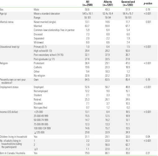
Characteristics including sex, age, marital status, education, religion, housing situation, employment status, income, num-ber of children and adults living at home, and being a native of the country studied (Canada/Australia) were analyzed (Table 1).
Alcohol Consumption and Hazardous Alcohol Use
Patterns of alcohol consumption were assessed using the Alcohol Use Disorder Identification Test (AUDIT) [14] in which the participants were asked about their alcohol consumption (i.e., frequency, quantity) during the previous 30 days. Among people who reported consuming at least 1 drink of any alco-holic beverage during the past 30 days, further questions about alcohol consumption were formulated and recoded based on the AUDIT score as following:a) Number of DAYS on which you had a least one drink of any alcohol beverage during the past 30 days. It was codified as 0, none; 1, 1 day; 2, 2-4 days; 3, 5-15 days; and 4, 16-30 days; b) On the days when you drank, number of DRINKS on average during the past 30 days? It was codified as 0, 0-2 drinks; 1, 3-4 drinks; 2, 5-6 drinks; 3, 7-9 drinks; and 4, if ≥10 drinks; and c) Considering all types of alcoholic beverages, number of TIMES during the past 30 days you had 6 or more drinks on an occasion? It was codified as 0, none; 2, 1-7 times; 3, 8-12 times; and 4, if ≥13 times.
Hazardous alcohol use was calculated adding the scores giv-en above (a+b+c). It was considered positive if the resulting score was ≥3 in females and ≥4 in males.
Statistical Analysis
Descriptive statistics were used to present the demographic findings and patterns of alcohol consumption and alcohol risk among the study populations (Alberta and Queensland) and among the population groups with alcohol risk. Percentages were used for categorical variables and means (standard devi-ations [SD]) for continuous variables. The chi-square test or Student t-test was used to analyze the differences in the distri-bution of the variables between the 2 populations. Associa-tions between hazardous alcohol use and demographic char-acteristics among Albertans and Queenslanders were ana-lyzed through multivariate logistic regression analyses.
Statistical significance was accepted for p-values <0.05. All analyses were performed using SPSS version 23.0 (IBM Corp., Armonk, NY, USA).
RESULTS
Descriptive Findings
was 41.2%. In both groups studied, there was oversampling in the 55 and above age categories, and undersampling in the under-35 age categories. Otherwise, the demographics of the participants reasonably approximated the general population. Approximately half of the population included in the study were males (50.6%), and the mean age of the whole study group was 54.5 years (SD, 16.1 years). Albertans were
[image:4.595.45.554.86.589.2]signifi-cantly younger (p<0.001) and had a higher educational level than Queenslanders (p<0.001). In addition, a higher percent-age of the participants from Alberta had no children living in the house (p=0.04) and were living alone (p<0.001) compared with participants from Queensland. The distribution of marital status, employment status, and income were also significantly different between both populations studied (Table 1).
Table 1. Description of the populations included in the study
All
(n=2500) (nAlberta =1207) Queensland (n=1293) p-value
Sex Male 50.6 49.3 51.9 0.19
Age (y) Mean±standard deviation 54.5±16.1 52.4±16.4 56.4±15.7 <0.001
Range 18-101 18-94 18-101
Marital status Never married (single) 13.1 14.6 11.7 0.001
Married 63.7 59.4 67.7
Common-law relationship / live-in partner 5.9 6.4 5.4
Divorced 7.3 8.8 6.0
Separated 2.0 2.2 1.9
Widowed 8.0 8.6 7.4
Educational level (y) Primary (0-7) 1.0 0.4 1.5 <0.001
High school (8-13) 39.4 28.2 50.0
Post-secondary school (14-16) 32.1 37.9 26.7
Post-graduate (≥17) 27.4 33.5 21.8
Religion Protestant 38.4 29.1 47.0 <0.001
Catholic 19.6 20.3 18.9
Other 9.4 18.3 1.2
No religion 32.6 32.2 32.9
Presently own or rent your
residence? Own 84.5 83.5 85.4 0.19
Employment status Employed 52.6 56.7 48.8 <0.001
Not employed 12.2 9.0 15.1
Student 2.1 3.3 1.0
Retired 25.3 26.1 24.6
Disabled 7.1 3.7 10.3
Not specified 0.7 1.2 0.2
Income (US dollar) <25 000 13.1 8.4 18.5 <0.001
25 000-49 999 15.5 12.5 18.9
50 000-74 999 14.7 16.2 13.1
75 000-99 000 12.3 13.3 11.1
100 000-124 999 14.6 15.7 13.5
≥125 000 29.8 33.9 24.9
Children living in household Yes 31.1 29.1 33.0 0.04
No. of adults living in household (including
the participant)
1 2.2 22.0 16.1 <0.001
2 1.0 56.0 62.7
≥3 1.1 22.0 21.2
Born in Canada / Australia Yes 79.0 80.1 78.0 0.21
Alcohol Consumption
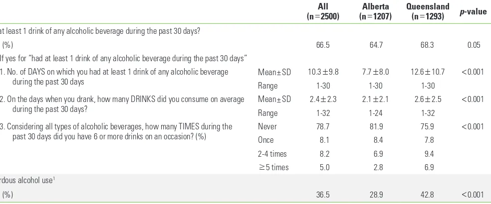
Sixty-five percent of Albertans and 68% of Queenslanders reported having had at least 1 drink of any alcoholic beverage during the past 30 days (p=0.052). Queenslanders reported having alcohol on more days during the past 30 days (p<
0.001), when drinking, drank more alcoholic beverages on av-erage (p<0.001), and were more likely to have had 6 or more drinks on a given occasion (p<0.001) than Albertans. Conse-quently, Queenslanders showed a higher level of hazardous alcohol use than Albertans (p<0.001) (Table 2).
Factors Associated With Alcohol Risk in Both
Populations Studied
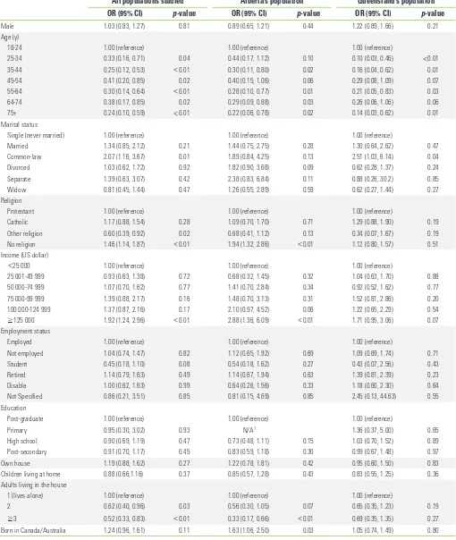
Hazardous alcohol use was associated with being between 18 and 24 years of age (Table 3), having common-law marital sta-tus (odds ratio [OR], 2.07; 95% CI, 1.16 to 3.67; p=0.01), having no religion (OR, 1.46; 95% CI, 1.14 to 1.87; p=0.003), and having an income of ≥$125 000 (OR, 1.92; 95% CI, 1.24 to 2.96; p=
0.003). Conversely, lower rates of hazardous alcohol use were associated with reporting a non-Catholic or Protestant religious affiliation (OR, 0.60; 95% CI, 0.39 to 0.92; p=0.02) and with liv-ing with 1 (OR, 0.62; 95% CI, 0.40 to 0.96; p=0.03) or more (OR, 0.52; 95% CI, 0.33 to 0.83; p=0.006) adults in the house.
Factors Associated With Alcohol Risk in Albertans
In the population of Alberta, hazardous alcohol use was as-sociated with being between 18 and 24 years of age (Table 3),having no religion (OR, 1.94; 95% CI, 1.32 to 2.86; p=0.001), having an income of ≥$125 000 (OR, 2.88; 95% CI, 1.36 to 6.09; p=0.006) and being born in Canada (OR, 1.63; 95% CI, 1.06 to 2.50; p=0.03). Living with 2 or more adults in the house was associated with lower rates of hazardous alcohol use (OR, 0.33; 95% CI, 0.17 to 0.66; p=0.002).
Factors Associated With Alcohol Risk in
Queenslanders
In a crude regression model, male Queenslanders were more likely to exhibit hazardous alcohol use than females (OR, 1.47; 95% CI, 1.18 to 1.84; p=0.001). However, the significance of the association between sex and hazardous alcohol use dis-appeared once additional relevant demographic variables were incorporated into the multivariate analysis (p=0.21) (Ta-ble 3). Among the population of Queensland, hazardous alco-hol use was associated with being between 18 and 24 years of age (Table 3) and having common-law marital status (OR, 2.51; 95% CI, 1.03 to 6.14; p=0.04).
DISCUSSION
A higher rate of hazardous alcohol use was found in Queenslanders than in Albertans, and a different combination of socio-demographic factors was associated with hazardous alcohol use in each of those populations. To the best of our knowledge, this is one of the first studies to use a common ap-Table 2. Alcohol consumption and hazardous alcohol use
All
(n=2500) (nAlberta =1207) Queensland (n=1293) p-value Had at least 1 drink of any alcoholic beverage during the past 30 days?
Yes (%) 66.5 64.7 68.3 0.05
If yes for “had at least 1 drink of any alcoholic beverage during the past 30 days” 1. No. of DAYS on which you had at least 1 drink of any alcoholic beverage
during the past 30 days Mean±SD 10.3
±9.8 7.7±8.0 12.6±10.7 <0.001
Range 1-30 1-30 1-30
2. On the days when you drank, how many DRINKS did you consume on average
during the past 30 days? Mean±SD 2.4
±2.3 2.1±2.1 2.6±2.5 <0.001
Range 1-32 1-24 1-32
3. Considering all types of alcoholic beverages, how many TIMES during the
past 30 days did you have 6 or more drinks on an occasion? (%) NeverOnce 78.78.1 81.98.4 75.97.8 <0.001
2-4 times 8.2 6.9 9.4
≥5 times 5.0 2.8 6.9
Hazardous alcohol use1
Yes (%) 36.5 28.9 42.8 <0.001
SD, standard deviation.
[image:5.595.60.552.86.291.2]Table 3. Associations between hazardous alcohol use and socio-demographic characteristics
All populations studied Alberta’s population Queensland’s population OR (95% CI) p-value OR (95% CI) p-value OR (95% CI) p-value
Male 1.03 (0.83, 1.27) 0.81 0.89 (0.65, 1.21) 0.44 1.22 (0.89, 1.66) 0.21
Age (y)
18-24 1.00 (reference) 1.00 (reference) 1.00 (reference)
25-34 0.33 (0.16, 0.71) 0.04 0.44 (0.17, 1.12) 0.10 0.10 (0.03, 0.46) <0.01
35-44 0.25 (0.12, 0.53) <0.01 0.30 (0.11, 0.80) 0.02 0.16 (0.04, 0.62) 0.01
45-54 0.41 (0.20, 0.85) 0.02 0.40 (0.15, 1.06) 0.06 0.29 (0.08, 1.09) 0.07
55-64 0.30 (0.14, 0.64) <0.01 0.28 (0.10, 0.77) 0.01 0.21 (0.05, 0.83) 0.03
64-74 0.38 (0.17, 0.85) 0.02 0.29 (0.09, 0.88) 0.03 0.26 (0.06, 1.06) 0.06
75+ 0.24 (0.10, 0.59) <0.01 0.22 (0.06, 0.78) 0.02 0.14 (0.03, 0.62) 0.01
Marital status
Single (never married) 1.00 (reference) 1.00 (reference) 1.00 (reference)
Married 1.34 (0.85, 2.12) 0.21 1.44 (0.75, 2.75) 0.28 1.30 (0.64, 2.62) 0.47
Common-law 2.07 (1.16, 3.67) 0.01 1.89 (0.84, 4.25) 0.13 2.51 (1.03, 6.14) 0.04
Divorced 1.03 (0.62, 1.72) 0.92 1.82 (0.90, 3.68) 0.09 0.62 (0.28, 1.37) 0.24
Separate 1.39 (0.63, 3.07) 0.42 2.38 (0.83, 6.84) 0.11 0.88 (0.26, 30.2) 0.85
Widow 0.81 (0.45, 1.44) 0.47 1.26 (0.55, 2.89) 0.59 0.62 (0.27, 1.44) 0.27
Religion
Protestant 1.00 (reference) 1.00 (reference) 1.00 (reference)
Catholic 1.17 (0.88, 1.54) 0.28 1.09 (0.70, 1.70) 0.71 1.29 (0.88, 1.90) 0.19
Other religion 0.60 (0.39, 0.92) 0.02 0.68 (0.41, 1.12) 0.13 0.34 (0.07, 1.67) 0.19
No religion 1.46 (1.14, 1.87) <0.01 1.94 (1.32, 2.86) <0.01 1.12 (0.80, 1.57) 0.51
Income (US dollar)
<25 000 1.00 (reference) 1.00 (reference) 1.00 (reference)
25 001-49 999 0.93 (0.63, 1.38) 0.72 0.68 (0.32, 1.45) 0.32 1.04 (0.63, 1.70) 0.88
50 000-74 999 1.07 (0.70, 1.62) 0.77 1.41 (0.70, 2.84) 0.34 0.92 (0.52, 1.62) 0.77
75 000-99 999 1.39 (0.88, 2.17) 0.16 1.48 (0.70, 3.13) 0.31 1.52 (0.81, 2.86) 0.20
100 000-124 999 1.37 (0.87, 2.16) 0.17 2.10 (0.97, 4.52) 0.06 1.22 (0.65, 2.29) 0.54
≥125 000 1.92 (1.24, 2.96) <0.01 2.88 (1.36, 6.09) <0.01 1.71 (0.95, 3.06) 0.07
Employment status
Employed 1.00 (reference) 1.00 (reference) 1.00 (reference)
Not employed 1.04 (0.74, 1.47) 0.82 1.12 (0.65, 1.92) 0.69 1.09 (0.69, 1.74) 0.71
Student 0.45 (0.18, 1.10) 0.08 0.54 (0.18, 1.62) 0.27 0.43 (0.07, 2.56) 0.43
Retired 1.14 (0.79, 1.63) 0.49 1.14 (0.67, 1.94) 0.63 1.39 (0.81, 2.39) 0.23
Disable 1.00 (0.62, 1.63) 0.99 0.64 (0.26, 1.56) 0.33 1.18 (0.60, 2.30) 0.64
Not Specified 0.86 (0.21, 3.51) 0.85 0.81 (0.15, 4.69) 0.85 2.45 (0.13, 44.63) 0.55
Education
Post-graduate 1.00 (reference) 1.00 (reference) 1.00 (reference)
Primary 0.95 (0.30, 3.02) 0.93 N/A1 1.36 (0.37, 5.00) 0.65
High school 0.90 (0.69, 1.19) 0.47 0.73 (0.48, 1.11) 0.15 1.03 (0.70, 1.52) 0.89
Post-secondary 0.91 (0.70, 1.17) 0.45 0.83 (0.59, 1.18) 0.30 0.99 (0.67, 1.48) 0.97
Own house 1.19 (0.88, 1.62) 0.27 1.22 (0.78, 1.81) 0.42 0.95 (0.60, 1.50) 0.83
Children living at home 0.88 (0.66,1.16) 0.37 0.85 (0.57, 1.28) 0.43 0.83 (0.55, 1.25) 0.36
Adults living in the house
1 (lives alone) 1.00 (reference) 1.00 (reference) 1.00 (reference)
2 0.62 (0.40, 0.96) 0.03 0.56 (0.30, 1.05) 0.07 0.65 (0.35, 1.23) 0.19
≥3 0.52 (0.33, 0.83) <0.01 0.33 (0.17, 0.66) <0.01 0.69 (0.35, 1.35) 0.27
Born in Canada/Australia 1.24 (0.96, 1.61) 0.11 1.63 (1.06, 2.50) 0.03 1.05 (0.74, 1.49) 0.80
Multivariate logistic regression analyses used alcohol risk as the dependent variable. OR, odds ratio; CI, confidence interval; N/A, not applicable.
proach to compare alcohol consumption and factors associat-ed with it between 2 populations from different countries.
A similar percentage of Albertans and Queenslanders re-ported having consumed alcohol during the past month. However, based on an analysis of patterns of alcohol con-sumption, we found that Queenslanders showed a higher rate of hazardous alcohol use than Albertans. This finding is not particularly surprising, due to the fact that higher alcohol con-sumption per capita has been described in Australia than in Canada [8]. Availability-limitations policies, implemented by increasing the price of alcohol and regulating the context (places or times) where consumers can obtain alcohol, have proven to be cost-effective ways to control alcohol consump-tion [15]. From the perspective of context, based on the infor-mation presented in the introduction about alcohol taxes and the number of alcohol licenses per population in Alberta and Queensland, we can infer that affordability (lower costs) may have a greater influence on hazardous alcohol consumption than availability (more licenses). However, further studies comparing the effects of alcohol policy on hazardous alcohol consumption between countries are needed.
In the overall population studied, hazardous alcohol use was associated with being between 18 and 24 years of age. This finding is in line with a previous study that established that mean alcohol consumption rose sharply during adolescence, peaked at around 25 years, and then declined and plateaued during mid-life [16]. In addition, our study found no difference in hazardous alcohol use by educational level; however, higher income was associated with hazardous alcohol use, in accor-dance with previous evidence [17]. These results are likely relat-ed to the high incomes earnrelat-ed by those working in the resource sectors in both countries, which have agricultubased and re-source-based economies. Workers in the oil and gas industries in Alberta [18] and in the mining industry in Queensland [19] have higher average earnings than those in other industries. In addition, the cyclic nature of those jobs, with long periods of rest vs. periods of intense work, combined with the isolated lo-cation of the workplaces, might be possible work stress factors influencing higher alcohol consumption [20]. Further studies are needed to confirm this hypothesis and its implications.
Other socio-demographic characteristics such as having no religion, living alone, and being born in Canada were also as-sociated with hazardous alcohol use among Albertans. Previ-ous research has suggested religiosity as protective factor against the early onset of alcohol use and later development
of alcohol problems [21]. Loneliness, probably due to the modern way of living in industrialized societies, has also been recognized as a cause and consequence of alcohol abuse [22]. Greater alcohol-related problems have been reported among Canadian-born individuals than among immigrants [23], per-haps as a consequence of other factors, such as better socio-economic status.
In Queenslanders, hazardous alcohol use was also associat-ed with common-law marital status. Previous studies have found lower alcohol consumption in married and common-law people, when grouped into a single category, than among single or divorced individuals [24,25]. However, we found that the patterns of alcohol consumption seemed to be different in common-law couples than in married people, and therefore these groups should be explored separately.
Lower rates of hazardous alcohol use was found among those having a religious affiliation other than Catholic or Prot-estant when the overall population was analyzed. Evidence has shown that Mormons, Jews, and Muslims are less likely to use alcohol than Catholics and liberal Protestants [26,27]. This association was not significant in Alberta or Queensland when analyzed separately, probably due to the small numbers of people with non-Catholic or Protestant religious affiliation in each population.
The homogenous design and implementation of data col-lection constitute a key strength of the present research. To the best of our knowledge, this is the first study to compare alcohol consumption between regions of 2 different, yet com-parable, countries. An additional strength of the present study was the analysis of the specific socio-demographic character-istics associated with hazardous alcohol use in each of the populations studied.
the fact that this demographic group has been particularly af-fected by the shift towards exclusive use of mobile phones.
This study presents the key socio-demographic factors asso-ciated with hazardous alcohol use in the populations of Alber-ta and Queensland. These results can be used by health plan-ners and policymakers to design and implement strategies de-signed to reduce hazardous alcohol use in those populations. From a policy perspective, it is important to consider that poli-cies with the goal of controlling alcohol consumption by af-fecting its cost (i.e., taxes and volumetric pricing) are more likely to impact populations with lower incomes, which have already a lower rate of hazardous alcohol use, whereas popula-tions with higher incomes are less likely to be affected. Conse-quently, efforts should be directed to the identification of more effective ways to tackle alcohol use in the higher-income group, which could be harder to reach through some of the traditional methods used to control alcohol consumption. Par-ticular care should be taken when considering the potential effect of raising alcohol prices on alcohol consumption among younger adults. Although it is possible that a substantial in-crease in the price of alcohol could help to restrict the con-sumption of alcohol in this population group, higher alcohol prices can also lead to the consumption of other recreational drugs prior to (or in combination with) alcohol intake, increas-ing the potential risk of injuries or other health problems.
The comparison of alcohol-related policies between both lo-cations is outside the scope of this study. Nevertheless, based on the fact that the mark-up rate of alcohol in Queensland seems to be lower than in Alberta and the oppose pattern was found in hazardous alcohol use, we speculate that alcohol-re-lated policies that impact affordability by increasing alcohol prices could have a positive effect in those regions despite their overall high socioeconomic status. Overall, current and novel strategies should be planned according to the character-istics of the population exhibiting hazardous alcohol use in each context.
In conclusion, younger age was associated with hazardous alcohol use in both populations. In addition, different socio-demographic factors were associated with hazardous alcohol use in each of the populations studied. Our results allowed us to identify the socio-demographic profiles associated with hazardous alcohol use in Alberta and Queensland. These pro-files constitute valuable sources of information for local health authorities and policymakers when designing suitable preven-tive strategies targeting alcohol use. Overall, the present study
highlights the importance of analyzing the socio-demograph-ic factors associated with alcohol consumption in population-specific contexts.
ACKNOWLEDGEMENTS
The authors acknowledge the Population Research Labora-tories of the Department of Sociology at the University of Al-berta and the Institute for Health and Social Science Research at Central Queensland University for their assistance with data collection.
CONFLICT OF INTEREST
The authors have no conflicts of interest associated with the material in this paper.
ORCID
Diana C. Sanchez-Ramirez http://orcid.org/0000-0003-1637-4309
Richard Franklin http://orcid.org/0000-0003-1864-4552
REFERENCES
1. World Health Organization. Global status report on alcohol and health 2014 [cited 2016 Jul 5]. Available from: http://apps. who.int/iris/bitstream/10665/112736/1/9789240692763_ eng.pdf.
2. Bloomfield K, Stockwell T, Gmel G, Rehn N. International com-parisons of alcohol consumption. Alcohol Res Health 2003;27 (1):95-109.
3. Rehm J, Rehn N, Room R, Monteiro M, Gmel G, Jernigan D, et al. The global distribution of average volume of alcohol con-sumption and patterns of drinking. Eur Addict Res 2003;9(4): 147-156.
4. Howard SJ, Gordon R, Jones SC. Australian alcohol policy 2001-2013 and implications for public health. BMC Public Health 2014;14:848.
6. Statistics Canada. Population by year, by province and territo-ry; 2016 [cited 2016 Jul 5]. Available from: http://www.statcan. gc.ca/tables-tableaux/sum-som/l01/cst01/demo02a-eng.htm. 7. Queensland Government. Population growth, Queensland,
December quarter 2014; 2015 [cited 2016 Jul 5]. Available from: http://www.qgso.qld.gov.au/products/reports/index. php.
8. Organization for Economic Cooperation and Development. Tackling harmful alcohol use: economics and public health policy; 2015 [cited 2016 Jul 5]. Available from: http://iogt.org/ wp-content/uploads/2015/03/OECD-report-2015.pdf. 9. Alberta Gaming and Liqour Commission (AGLC). AGLC survey
of Albertans 2015 [cited 2017 Sep 14]. Available from: https:// aglc.ca/sites/aglc.ca/files/aglc_files/quickfacts_liquor.pdf. 10. Alberta Gaming and Liquor Commission (AGLC). Alcohol
mark-up rate schedule [cited 2017 Sep 14]. Available from: https:// www.cfta-alec.ca/wp-content/pdfs/English/DisputeResolu- tion/Beer/25-Alberta-Liquor-and-Gaming-Commission-Mark-up-Rate-Schedule-Effective-August-5-2016.pdf.
11. Australian Institute of Health and Welfare. 2010 National drug strategy household survey; 2011 [cited 2016 Jul 5]. Available from: http://www.aihw.gov.au/WorkArea/DownloadAsset. aspx?id=10737421314.
12. Department of Justice and Attorney-General. Liquor statistics [cited 2016 Jul 5]. Available from: http://www.justice.qld.gov. au/corporate/business-areas/liquor-gaming/liquor/statistics. 13. Australian Taxation Office. Excise rates for alcohol [cited 2016
Jul 5]. Available from: https://www.ato.gov.au/Business/Ex- cise-and-excise-equivalent-goods/Alcohol-excise/Excise-rates-for-alcohol/.
14. Babor TF, Higgins-Biddle J, Saunders JB, Monteiro MG. AUDIT, the alcohol use disorders identification test: guidelines for use in primary care. 2nd ed. Geneva: World Health Organization; 2001, p. 19.
15. Babor TF, Caetano R, Casswell S, Edward G, Giesbrecht N, Gra-ham K, et al. Alcohol: no ordinary commodity: research and public policy. 2nd ed. New York: Oxford University Press; 2010, p. 103-146.
16. Britton A, Ben-Shlomo Y, Benzeval M, Kuh D, Bell S. Life course trajectories of alcohol consumption in the United Kingdom using longitudinal data from nine cohort studies. BMC Med 2015;13:47.
17. Keyes KM, Hasin DS. Socio-economic status and problem al-cohol use: the positive relationship between income and the DSM-IV alcohol abuse diagnosis. Addiction 2008;103(7):1120-1130.
18. Alberta Learning Information Service. Oil and gas well drilling and related workers and services operators [cited 2017 Aug 8]. Available from: https://occinfo.alis.alberta.ca/occinfopreview/ info/browse-wages/wage-profile.html?id=8412.
19. Australian Bureau of Statistics. Employee earnings, benefits and trade union membership, Australia, August 2013; 2014 [cited 2016 Jul 5]. Available from: http://www.abs.gov.au/aus-stats/abs@.nsf/mf/6310.0.
20. Frone MR. Work stress and alcohol use. Alcohol Res Health 1999;23(4):284-291.
21. Porche MV, Fortuna LR, Wachholtz A, Stone RT. Distal and proximal religiosity as protective factors for adolescent and emerging adult alcohol use. Religions (Basel) 2015;6(2):365-384.
22. Akerlind I, Hörnquist JO. Loneliness and alcohol abuse: a re-view of evidences of an interplay. Soc Sci Med 1992;34(4):405-414.
23. Auger N, Hamel D, Martinez J, Ross NA. Mitigating effect of immigration on the relation between income inequality and mortality: a prospective study of 2 million Canadians. J Epide-miol Community Health 2012;66(6):e5.
24. Chilcoat HD, Breslau N. Alcohol disorders in young adulthood: effects of transitions into adult roles. J Health Soc Behav 1996;37(4):339-349.
25. Curran PJ, Muthén BO, Harford TC. The influence of changes in marital status on developmental trajectories of alcohol use in young adults. J Stud Alcohol 1998;59(6):647-658.
26. Bartkowski JP, Xu X. Religiosity and teen drug use reconsid-ered: a social capital perspective. Am J Prev Med 2007;32(6 Suppl):S182-S194.
27. Michalak L, Trocki K, Bond J. Religion and alcohol in the U.S. National Alcohol Survey: how important is religion for absten-tion and drinking? Drug Alcohol Depend 2007;87(2-3):268-280.