Statistical Approaches for Signal Processing with Application to Automatic Singer Identification

Theses

Thesis/Dissertation Collections

6-2016

Statistical Approaches for Signal Processing with

Application to Automatic Singer Identification

Shiteng Yang

[email protected]

Follow this and additional works at:

http://scholarworks.rit.edu/theses

This Thesis is brought to you for free and open access by the Thesis/Dissertation Collections at RIT Scholar Works. It has been accepted for inclusion in Theses by an authorized administrator of RIT Scholar Works. For more information, please [email protected].

Recommended Citation

M

THESIS

Statistical Approaches for Signal

Processing with Application to

Automatic Singer Identification

Author:

Shiteng YANG

Supervisor:

Dr. Ernest FOKOUÉ

A thesis submitted in partial fulfillment of the requirements for the degree of Master of Science in Applied Statistics

in the

Applied Statistics Graduate Program School of Mathematical Sciences

College of Science

Ernest Fokoué

, Associate Professor, School of Mathematical Sciences

Date

Thesis Advisor

Joseph Voelkel

, Professor, School of Mathematical Sciences

Date

Committee Member

Declaration of Authorship

I, Shiteng YANG, declare that this thesis titled, “Statistical Approaches for

Sig-nal Processing with Application to Automatic Singer Identification” and the work presented in it are my own. I confirm that:

• This work was done wholly or mainly while in candidature for a research degree at this University.

• Where any part of this thesis has previously been submitted for a degree or any other qualification at this University or any other institution, this has been clearly stated.

• Where I have consulted the published work of others, this is always clearly attributed.

• Where I have quoted from the work of others, the source is always given. With the exception of such quotations, this thesis is entirely my own work.

• I have acknowledged all main sources of help.

• Where the thesis is based on work done by myself jointly with others, I have made clear exactly what was done by others and what I have contributed myself.

Signed:

“Thanks to my solid academic training, today I can write hundreds of words on virtually any topic without possessing a shred of information, which is how I got a good job in journalism.”

ROCHESTER INSTITUTE OF TECHNOLOGY

Abstract

Ernest Fokoué

School of Mathematical Sciences

Master of Science in Applied Statistics

Statistical Approaches for Signal Processing with Application to Automatic Singer Identification

by Shiteng YANG

Acknowledgements

I would first like to thank my thesis advisor Prof. Ernest Fokoué for the contin-uous support of my MS study and related research, for his patience, motivation, and immense knowledge. His guidance helped me in all the time of research and writing of this thesis. The door to his office was always open whenever I ran into a trouble spot or had a question about my research or writing. He consistently al-lowed this paper to be my own work, but steered me in the right direction when-ever he thought I needed it. I could not have imagined having a better advisor and mentor for my MS study.

Besides my advisor, I would like to thank the rest of my thesis committee: Prof. Joseph Voelkel and Prof. Peter Bajorski, for their insight comments and encour-agement, but also for the hard question which incented me to widen my research from various perspectives.

Finally, I must express my very profound gratitude to my parents for providing me with unfailing support and continuous encouragement throughout my years of study and through the process of researching and writing this thesis. This ac-complishment would not have been possible without them. Thank you.

Contents

Declaration of Authorship i

Abstract iii

Acknowledgements iv

1 Introduction 1

1.1 Background . . . 1

1.1.1 The attribute of singing voice . . . 2

1.1.2 Singer identification and speaker recognition . . . 2

1.1.3 Auditory features . . . 3

1.1.4 Other researchers’ works on singer identification . . . 4

1.1.5 Contribution . . . 4

1.2 Thesis Organization. . . 4

2 Feature Extraction Techniques 6 2.1 Principal Component Analysis . . . 6

2.1.1 PCA via Eigenvalue Decomposition . . . 7

2.1.2 PCA and Singular Value Decomposition . . . 9

2.1.3 PCA of High-dimension and Low-sample-size . . . 10

2.2 Mel-frequency Cepstral Coefficient . . . 11

2.2.1 Pre-emphasis . . . 12

2.2.2 Frame Blocking . . . 13

2.2.3 Hamming Windowing . . . 13

2.2.4 Fourier Transform . . . 15

2.2.5 Mel Filter Bank Processing . . . 16

2.2.6 Discrete Cosine Transform. . . 19

3 Classification Technique 20 3.1 Support Vector Machine . . . 20

3.1.1 Binary SVM . . . 21

3.1.2 Multi-Class SVM . . . 25

3.2 Gaussian Mixture Model . . . 27

3.2.1 K-means Clustering . . . 29

3.2.2 EM Algorithm. . . 31

4 Singing Voice Detection and Separation 34 4.1 Singing Voice Detection . . . 35

4.1.1 Traditional Method - Double GMM . . . 35

4.1.2 Improved Method - Single GMM . . . 37

4.2 Singing Voice Separation . . . 38

4.2.1 Non-negative Matrix Factorization . . . 39

5 Implementation of Automatic Singer Identification 46

5.1 Auto-SID Overview. . . 46

5.1.1 System Configuration . . . 46

5.1.2 Singer Classifier. . . 47

5.2 Dataset Introduction . . . 48

5.2.1 Music Recordings Collection . . . 48

5.2.2 Source Matrix Construction and Feature Matrix Selection. . 49

5.3 Experiments and Results of Pre-processing Techniques . . . 51

5.3.1 Singing Voice Detection - Double and Single GMM . . . 51

5.3.2 Singing Voice Separation - NMF and RPCA . . . 53

5.4 Experiments and Results of Singer Identification . . . 54

5.4.1 Analysis on Time Domain - PCA . . . 54

5.4.2 Analysis on Frequency Domain - MFCC . . . 57

5.4.3 Source Matrix Type Comparison . . . 58

5.4.4 Testing Segment Length Comparison . . . 59

5.4.5 Auto-SID with or without Singing Voice Separation . . . 60

5.5 Conclusion . . . 60

A Seleted Code 63 A.1 R Code in Performing Singing Voice Detection . . . 63

A.2 Matlab Code in Performing Background Music Removal . . . 67

List of Figures

2.1 Block diagram of the MFCCs calculation . . . 12

2.2 The effect of pre-emphasis . . . 13

2.3 Hamming Window . . . 14

2.4 Effect of multiplying a hamming window . . . 15

2.5 An example of Fourier Transform. . . 17

2.6 The transform between mel-scale and hertz-scale. . . 18

2.7 Example of triangular filter bank . . . 18

3.1 The maximum-margin separating hyperplane . . . 22

3.2 The decision boundary in the non-linear SVM . . . 24

3.3 Comparison of distribution modeling . . . 29

3.4 Demonstration of K-means clustering . . . 31

4.1 The block diagram of double GMM. . . 36

4.2 The block diagram of single GMM . . . 37

4.3 Spectrum of a music clips . . . 41

4.4 An example of components decomposed by NMF . . . 42

4.5 The spectrogram of WH after component selection . . . 43

4.6 Example RPCA results . . . 45

4.7 The block diagram of RPCA . . . 45

5.1 The block diagram of Auto-SID system . . . 47

5.2 The difference of the MFCC features between non-vocal and vocal segments . . . 52

5.3 Example of the RPCA separated audio tracks . . . 54

5.4 The pattern of prediction accuracy on time domain . . . 56

5.5 The effect of different number of PCs on MPA. . . 57

List of Tables

5.1 Singers and Albums . . . 49

5.2 Example of the source matrix . . . 50

5.3 Detection accuracy comparison . . . 52

5.4 The evaluation results of NMF and RPCA . . . 53

5.5 Number of Principal Components . . . 55

5.6 Training performance on time domain . . . 55

5.7 Testing accuracy comparison . . . 56

5.8 The singer identification performance on frequency domain . . . . 58

5.9 Comparison of source matrix type . . . 59

5.10 Comparison of testing length . . . 60

Chapter 1

Introduction

1.1

Background

As the digital music becoming more and more popular, music databases, both professional and personal, are growing fast. Technologies are needed for effi-ciently categorizing and retrieving these music collections, so that customers can be provided with powerful functions for browsing and searching musical content. The singer identification is such a technique that can be employed to identify the singer of a song by analyzing the auditory features of the music signal ([Kim and Whitman,2002],[Liu and Huang,2002]). With this capability involved in a music system, the users can easily get to know the singer’s information of an arbitrary song, or retrieve all songs performed by a particular singer in a distributed music database [(Zhang and Packard,2003)].

Searching for songs using the singer’s name is the most common method in mu-sic retrieval system. However, till now, the mumu-sic information retrieval system is based on text tags of singer’s names and song titles, not on characteristics of his or her voice. If the singer’s name is not known, a user could hardly find songs he wants. Hence, study based on using vocal segment in a song for retrieval is rather necessary [(Zhang and Packard,2003)]. A more direct way of singer identifica-tion is to retrieve the names of singers through the singer’s voice ([Fujihara et al.,

2010]). Furthermore, this technology can also be used to cluster songs of similar voices of singers in a music collection, or search for songs which are similar to a query song in terms of the singer’s voice.

in which the company will typically not have a copy of the original audio data for comparison.

1.1.1 The attribute of singing voice

The singing voice is the oldest musical instrument and one with which almost everyone has a great deal of familiarity ([Rao, Ramakrishnan, and Rao, 2009]). Given the importance and usefulness of vocal communication, it is not surprising that our auditory physiology and perceptual apparatus has evolved to a high level of sensitivity to the human voice. Once we are exposed to the sound of a particular person’s speaking voice, it is relatively easy to identify that voice, even with very little training. For the most part the same holds true with regards to the singing voice. Once we become familiar with the sound of a particular singer’s voice, we can usually identify the voice, even when hearing a piece for the first time. Not only is the voice the oldest musical instrument, it is also one of the most complex from an acoustic standpoint. This is primarily due to the rapid acoustic variation involved in the singing process. In order to pronounce different words, a singer must move their jaw, tongue, teeth, etc., changing the shape and thus the acoustic properties of their vocal tract. No other instrument exhibits the amount of physical variation of the human voice. This complexity has affected research in both analysis and synthesis of singing ([Kim,2001]).

In spite of this complexity, voice identification is almost effortless to us. But per-haps what is more remarkable is that even in the presence of interfering sounds, such as instruments or background noise, we can still identify the voice of a fa-miliar singer. Thus, our process of identification most likely depends on features invariant to these environmental variations.

1.1.2 Singer identification and speaker recognition

A significant amount of research has been performed on speaker recognition from digitized speech for applications such as verification of identity. These systems for the most part use features similar to those used in speech recognition. Many of these systems are trained on pristine data (without background noise) and per-formance tends to degrade in noisy environments. And since they are trained on spoken data, they perform poorly to singing voice input. For more on speaker recognition systems, see ([Mammone, Zhang, and Ramachandran,1996]).

distinguishing the characteristic features of one voice from another. The task of singer recognition is largely complicated because the singer’s voice is totally tangled with a non-stationary background signal ([Mammone, Zhang, and Ra-machandran,1996]). It is a difficult task to get original solo voice data (without background accompaniment) for directly extracting the singer’s vocal characteris-tics. Another important issue is caused by the requirement of training the system to differentiate between the various sound sources in the music recordings such as vocals, background accompaniments and background noises.

1.1.3 Auditory features

Singer identification belongs to artist identification in content-based Music Infor-mation Retrieval, there are many researches in this field and many research re-sults. Singer identification is mainly made up of two parts: feature extraction and classifier. Some methods are based on speech recognition, feature extrac-tion exemplified by Mel-frequency Cepstral Coefficient (MFCC) ([Zhang, 2003], [Khine, Nwe, and Li,2008], [Khine, Nwe, and Li,2007]), Liner Prediction Cepstral Coefficient (LPCC) ([Khine, Nwe, and Li,2007]), and models, by way of exam-ple, Gaussian Mixture Model (GMM) ([Chang,2009], [Fujihara et al.,2010]), Hid-den Markov Model (HMM) ([Nwe and Wang,2004]) and Support Vector Machine (SVM) ([Maddage, Xu, and Wang,2004]).

Recently, some new methods are proposed in feature extraction, for instance, Oc-tave Frequency Cepstral Coefficients (OFCC) ([Khine, Nwe, and Li, 2008]), Log Frequency Power Coefficients (LFPC) ([Nwe and Wang,2004]) and Timbre Cep-stral Coefficient ([Khine, Nwe, and Li,2007]). In ([Fujihara et al.,2010]), the ac-companiment sound is reduced using Goto’s PreFEst ([Goto,2004]) method, and LPMCCs and delta-F0s are employed as feature vectors. In ([Chang,2009]), pitch information is considered as features. In ([Bartsch and Wakefield,2004]), the vi-brato is extracted to identify the singing voice of human. However, this algo-rithm is affected by the accompaniment music. The researchers proposed that the non-negative matrix factorization (NMF) can be used to separate the singing voice from the accompaniment music in ([Chanrungutai and Ratanamahatana,

1.1.4 Other researchers’ works on singer identification

Many researches have been done on the field of singer identification mainly for music information retrieval systems. Kim et al. proposed a method to auto-matically determine the singer’s identity using the various acoustic attributes ex-tracted from songs ([Kim and Whitman,2002]). But this method failed to consider the impact of background music on the singer’s voice signal.

A method for singer identification based on spectrum, proposed by Bartsch and Wakefield, operated well only for ideal cases that contained the audio samples with singer’s voice only ([Bartsch and Wakefield,2004]).

In "Singer identification based on vocal and instrumental models" proposed by Maddageet al. the singer was identified using both low-level features and music structure knowledge ([Maddage, Xu, and Wang,2004]). But this method was not suitable for short test music recordings with more instrumental section.

Another method proposed by Fujiharaet al. was identifying the singer from poly-phonic musical audio signals including sounds of various instruments ([Fujihara et al.,2005]). But accurate melody extraction from polyphonic music was found to be a difficult task.

1.1.5 Contribution

Considering the existing researches in this thesis, we would like to propose new methods to resolve two fundamental problems. First, for singing voice detection, based on the traditional method known as double GMM which has been widely used by other researchers for many years, we propose an improved method known as single GMM which is proved to have better detection performance. Second, in order to remove the background music from the music recordings, we performed singing voice separation. Two statistical approaches are studied, Non-negative Matrix Factorization (NMF) and Robust Principal Component Analysis (RPCA). From the experimental result, it turns out that RPCA outperforms NMF.

1.2

Thesis Organization

Chapter 2

Feature Extraction Techniques

This chapter introduces two different methods for feature extraction: principle component analysis (PCA) and mel-frequency cepstral coefficient (MFCC). As we know, in digital signal processing, the data structure of high-dimension and low-sample-size (HDLSS) is always encountered. The analysis of HDLSS data can be performed by PCA and MFCC in the way of feature extraction. On the other hand, PCA is the method performed on the time domain, while MFCC is the technique implemented on the frequency domain.

Section 2.1 introduces the technique of principle component analysis. It is often used as a method to emphasize variation and extract out strong patterns in a data set. Although PCA is always regarded as a approach for multicollinearity rem-edy, essentially it can be used for feature extraction due to its distinct property in dimensionality reduction. Generally, principle components can be obtained via eigenvalue decomposition of XTX or singular value decomposition of X. But when HDLSS data structure shows up, these kinds of method can not be used any more sinceXTX is not singular in this case. In order to solve HDLSS problem, eigenvalue decomposition ofXXT is employed.

Section 2.2 introduces the method of mel-frequency cepstral coefficient. MFCC uses non-linear audio perception to mimic human listening features and is based upon the fact that human hearing perception can not perceive frequencies above 1000Hz. It performs the transformation for the signal from time domain to fre-quency domain and maps the transformed signal in hertz onto mel scale by using triangular overlapping windows. By now, MFCC is the most widely used feature extraction method for speech recognition system.

2.1

Principal Component Analysis

processing, multivariate quality control, mechanical engineering and etc ([Abdi and Williams,2010]).

PCA uses the orthogonal transformation to covert the correlated variables into the principle components that are linearly uncorrelated. The number of princi-ple components can be equal or less than the number of original variables. The importance of principle components is determined by the eigenvalues which can be used to measure the component ability on variation explanation ([Abdi and Williams,2010]). The first principle component has the largest eigenvalue which means that it has explained as much of the variability as possible, and all of the principle components are orthogonal to each other due to the reason that they are the eigenvectors of the symmetric covariance matrix.

The most important property of PCA is dimensionality reduction ([Richardson,

2009]). This property is very helpful for visualising and processing the datasets with very high dimensionality. Moreover, it is also reasonable to reduce the noise in the dataset through this method. If the variables in original matrix contain the gaussian noise which is independently identical distributed, then the princi-ple components in transformed matrix will also contain the noise with same at-tribute. The signal to noise ratio in the first few principle components which have a large proportion of variance will be very high. This is due to the fact that these components have explained most of the variability in the dataset, while the noise variance in each column stayed the same. Therefore, PCA can concentrate most of the signal into the first few principle components. The later components can be discarded without great loss since the signal to noise ratios in these components are very low.

2.1.1 PCA via Eigenvalue Decomposition

Principle component analysis can be performed by eigenvalue decomposition of

XTX, e.g. ([Jolliffe,2002]). Specifically, suppose that we have a datasetXn×pwith

nobservations andpvariables, heren > pand each column is centered at 0. Each row represents a different repetition of the experiment, and each column in the matrix is a random variable that gives a particular kind of feature.

Xn×p =

     

x11 x12 · · · x1p

x21 x22 · · · x2p

..

. ... . .. ...

xn1 xn2 · · · xnp

     

V ar(X) = Σ =      

σ₁2 σ12 · · · σ1p

σ21 σ22 · · · σ2p

..

. ... . .. ...

σp1 σp2 · · · σ2p

     

=E(X−E[X])T(X−E[X])

Since each variable in the dataset has been centered at 0, the equation showed above can be simplified to

V ar(X) =EXTX

And the corresponding sample variance-covariance matrix is

S= 1

n−1

     

xT₁x1 xT1x2 · · · xT1xp

xT₂x1 xT2x2 · · · xT2xp

..

. ... . .. ...

xT_px1 xTpx2 · · · xTpxp

      (2.1)

The above matrix is assumed to be positive definite and symmetric. The variance of each variable is located at the diagonal entry and the covariance between each two variables is located at the off-diagonal entry. In order to remedy the multi-collinearity, we linearly transform datasetX into a new dataset T in which the covariance between any two variables is exactly zero. The goal can be achieved by the way of eigenvalue decomposition of the matrixXTX([Jolliffe,2002]). The eigenvalues and eigenvectors of matrixXTX can be obtained through this equation:

XTX=WΛWT (2.2)

Here Λ = diag(λ1, λ2,· · · , λp) is ap×pdiagonal matrix in which the

eigenval-ues are located at the diagonal entry and λ1 ≥ λ2 ≥ · · · ≥ λp ≥ 0. W = [W1, W2,· · ·, Wp]is ap×porthogonal matrix, normally known as loading matrix,

in which the column vectorsWjare the eigenvectors. Moreover, each eigenvector

is subject to the constraint that

W_jTWj = p

X

i=1

Specifically, PCA performs the orthogonal linear transformation of datasetX in this way:

T1 =w11X1+w21X2+· · ·+wp1Xp=XW1

T2 =w12X1+w22X2+· · ·+wp2Xp=XW2

.. .

Tp =w1pX1+w2pX2+· · ·+wppXp =XWp

(2.3)

The variableTjin the transformed datasetT = [T1, T2,· · ·, Tp]is known as

princi-ple component and the covariance between each of component is equal to zero. So these principle components are linearly uncorrelated with each other. The equa-tion in 2.3can also be simplified to

T =XW (2.4)

There exists an important fact about this linear transformation that the trace of the matrixXTXis equal to the sum of the eigenvalues, e.g. ([Jolliffe,2002]). And also, notice that the trace is actually equal to the sum of variance of the variables in datasetXor transformed datasetT.

trace(XTX) = p

X

i=1

λi= (n−1) p

X

i=1

V ar(Xi) = (n−1) p

X

i=1

V ar(Ti) (2.5)

Therefore, based on the Equation 2.5and the fact thatλ1 ≥λ2 ≥ · · · ≥λp ≥0, it

is rarely necessary to keep all the principal components. Generally, we only keep the first L principle components which preserve 95% variation. The remaining components will be discarded without great information loss. This will gives a truncated transformation, that is

TL=XWL (2.6)

Where the transformed matrixTLnow has n rows but only L columns.

2.1.2 PCA and Singular Value Decomposition

Specifically, the singular value decomposition can be performed in this way:

X =U SVT (2.7)

Here,Sis a rectangular diagonal matrix withnrows andpcolumns. The positive numberssilocated at the diagonal entry are known as the singular values ofX.U

is a square matrix ofn×nsize, the columns of which are known as the left singular vectors ofX. AndW is ap×pmatrix whose columns are called the right singular vectors ofX. Moreover, both left singular vectors and right singular vectors are orthogonal unit vectors ([Giordani,2014]).

Based on the Equation 2.7, the matrixXTXcan be written as

XTX=V SUTU SVT =V S2VT

Compared with the eigenvalue decomposition ofXT_{X, we can see that the right}

singular vectorsV of X are equivalent to the eigenvectorsW of XTX and the singular valuessiofXare equal to the square roots of the eigenvaluesλiofXTX.

Therefore, in the singular value decomposition, the transformed matrixT can be written as

T =XW =U SVTV =U S (2.8)

So each column vector ofT is calculated by one of the left singular vectors ofX

multiplied by the corresponding singular value.

2.1.3 PCA of High-dimension and Low-sample-size

The data matrixXused in the above subsection is assumed to have an > p struc-ture that the number of the observations is greater than the number of the vari-ables. So the matrixXTX is non-singular or known as full rank matrix. When the data matrix of high-dimension and low-sample-size shows up,XTX will be-come singular and PCA can not be performed by either eigenvalue decomposition ofXTXor singular value decomposition of Xunder this situation. Fortunately, HDLSS problem can be solved by the eigenvalue decomposition ofXXT ([Shen, Shen, and Marron,2013],[Yata and Aoshima,2015]).

The eigenvalues and eigenvectors ofXXT can be calculated by the equation

XXT _=UΛUT

⇓

XXTU =UΛ

Then by pre-multiplying both sides of Equation 2.9byXT, we have

(XTX)(XTU) = (XTU)Λ

LetZ =XTU, then

XTXZ =ZΛ

⇓

XTX=ZΛZT

(2.10)

From Equation 2.10, we can see that the matrixZis equivalent to the loading ma-trixW in the Equation 2.2. So the principal components can be obtained through

T =XZ=X(XTU) (2.11)

2.2

Mel-frequency Cepstral Coefficient

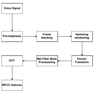
For any vocal signal recognition system, the first thing needed to be considered about is which method should be employed to extract the auditory features from signal. A good auditory feature should have the ability to extract out the com-ponent which carries information that can be used for identifying the linguis-tic message. By now, various feature extraction methods have been proposed, such as Linear Prediction Coefficients (LPC), Linear Prediction Cepstral Coeffi-cients (LPCC) ([Wong and Sridharan, 2001]), mel-frequency cepstral coefficients (MFCC) ([Logan et al.,2000]) and so on. And the most widely used features are mel-frequency cepstral coefficients (MFCCs). This extraction method was first mentioned by Bridle and Brown in 1974, further improved by Mermelste in 1976 and have been state of the art ever since ([Muda, Begam, and Elamvazuthi,2010]). The steps of the MFCCs calculation are showed as follows and can also be viewed visually in Figure2.1

• Step1: Pre-emphasis

• Step2: Frame blocking

• Step3: Hamming windowing

• Step4: Fourier transform

• Step5: Mel filter bank processing

FIGURE2.1: MFCC block diagram

2.2.1 Pre-emphasis

In the speech signal, the signal-to-noise ratio (SNR) in the low-frequency is actu-ally lower than the one in the high-frequency. Since the high-frequency band was suppressed during the sound production mechanism of humans, it is necessary to perform a preliminary analysis on the speech signal before transforming it from time domain to frequency domain, in order to increase the energy of signal at high frequency. This preliminary analysis is known as pre-emphasis. Specifically, a filter called first-order finite impulse response is used in this process, that is:

s2[n] =s[n]−a∗s[n−1] (2.12)

Here,s[n]is the input signal ands2[n]is the output. Moreover, whether this filter

FIGURE2.2: The effect of pre-emphasis withα= 0.95

2.2.2 Frame Blocking

Although the speech signal is time varying, its characteristics stay stationary in a sufficiently short period of time interval. For this reason, speech signal is pro-cessed in short time intervals. Specifically, the input speech signal is divided into frames of 20 to 50 ms and each frame overlaps its previous frame by a pre-defined size. The reason of overlapping is to smooth the transition from frame to frame. If the sampling rate is 16000 Hz and each frame has 320 sample points, then the frame length is320/16000 = 20ms. Moreover, if the pre-defined size of overlap-ping is 10 ms, then the frame rate is1000/10 = 100frames per second.

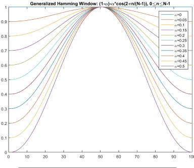
2.2.3 Hamming Windowing

function employed in MFCC is called hamming window function. The equation of this function is given by

w[n] = (1−α)−αcos

2πn

N −1

,0≤n≤N−1 (2.13)

Where N is the number of samples in each frame. Different values of α corre-sponds to different curves for the hamming windows as shown in the Figure 2.3.

FIGURE2.3: Hamming window with differentα

With the hamming window defined above, the result of windowing signal is shown below:

y[n] =s[n]×w[n] (2.14)

notice that the peak now become sharper and more distinct in the frequency re-sponse.

FIGURE2.4: Effect of multiplying a hamming window

2.2.4 Fourier Transform

Next, the frames obtained from previous step need to be transformed from time domain into frequency domain. This transformation process is performed by Fourier transform. This transform method is firstly introduced by Joseph Fourier in 1822 and has been playing a very important role in signal processing as a bridge between time domain and frequency domain.

Specifically, the equation of Fourier Transform can be written as

ˆ

f(ξ) =

Z ∞

−∞

f(x)e−2πixξdx (2.15)

eix=cosx+isinx

Equation 2.15shows the transform process from time domain to frequency do-main. And also, the inverse transform from frequency domain to time domain is given by

f(x) =

Z ∞

−∞

f(ξ)e2πiξxdξ (2.16)

Here,xcan be any real number.

Figure 2.5gives an example of Fourier transform. The signal used in this example has a very short time period. So this process can also be called short time fourier transform. Fourier transform can only be performed on the signal with a very short time period since the stationary assumption can not be satisfied on the signal with a long time period.

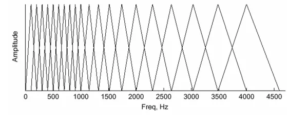
2.2.5 Mel Filter Bank Processing

The frequency is perceived by human ear in the non-linear way. Some researches have shown that the scaling is linear up to 1 kHz and logarithmic above that. The Mel-scale filter bank is a band pass filtering and can be used to characterize the human ear perceiveness of frequency. The signal in each frame obtained from previous steps is passed through Mel-scale band filter in order to modify and re-group it into some components and features.

Since the human perception of the frequency contents of sounds for speech sig-nals does not follow a linear scale, thus, instead of measuring frequency in Hz, a subjective pitch is measured on a scale called Mel-scale. This Mel-scale frequency is a linear frequency spacing below 1000 Hz and a logarithmic spacing above 1000 Hz. Moreover, Mel-frequency is proportional to the logarithm of the linear fre-quency, reflecting similar effects in the human’s subjective aural perception. As a reference point, the pitch with a 1000 Hz tone and 40 dB above the perceptual hearing threshold, is defined as 1000 mels. The transform between hertz-scale and mel-scale is give by

mel=

(

f f ≤1000

2595log10(1 +f /700) f >1000

(2.17)

FIGURE2.5: An example of Fourier Transform

A set of M triangular filters are used to calculate a weighted sum of filter spectral components so that the output of process is close to a Mel scale. Each filter’s magnitude frequency response is triangular in shape and equal to unity at the center frequency and decrease linearly to zero at center frequency of two adjacent filters. A triangular filter of lengthLcan be written as

Mm[l] = 1−

l−L−1 2 L−1

2

FIGURE2.6: The transform between mel-scale and hertz-scale

and the log energy of each triangular bandpass filter can be calculated by

E[m] =ln

" _L X

l=0

|xa[l]|2Mm[l]

#

, m= 1,2, ..., M (2.19)

The reason for using the triangular filter is that the magnitude spectrum, such that the harmonics are flattened, need to be smoothed in order to obtain the envelop of the spectrum with harmonics. This indicates that the pitch of a speech signal is generally not included in MFCC. As a result, when the input audio tracks have the same timbre but different tones, then, a speech recognition system will behave more or less the same. An example of triangular filter bank is given in Figure 2.7. Notice that as the frequency increases, the filters would cover a wider band and a short length of overlapping is needed to eliminate the discontinuity.

2.2.6 Discrete Cosine Transform

In this step, Discrete Cosine Transform (DCT) is applied on the M log energyE[m]

obtained from previous step to calculate MFCC. The formula of DCT can be writ-ten as

c[q] = M

X

m=1

E[m]cos

πq(m−0.5)

M

, q= 1,2,3, ... (2.20)

Chapter 3

Classification Technique

This chapter introduces two widely used statistical machine learning classification techniques: Support Vector Machine (SVM) and Gaussian Mixture Model (GMM). In the field of data analysis, machine learning is a method that can be used to create complex models or algorithms and make themselves to prediction. These models and algorithms make it available for researchers, data scientists, engineers and analysts to make reliable decisions and uncover hidden insights by learning from historical relationships and trends in the data.

Section 3.1 introduces support vector machine. It is a supervised learning algo-rithm that can be used for classification and regression analysis. Given a set of training data points, each labelled for belonging to one of two classes, an SVM training algorithm fits a model that assigns a new data point into one class or the other, making this algorithm a non-probabilistic binary linear classifier.

Section 3.2 introduces Gaussian mixture model. It is a parametric probability den-sity function represented as a weighted sum of Gaussian component densities. GMMs are commonly used as a parametric model of the probability distribution of continuous measurements or features in a biometric system, such as vocal-tract related spectral features in a speaker recognition system. Parameters of the GMMs are initialized via K-means clustering and iteratively adjusted via Expectation-Maximization (EM).

3.1

Support Vector Machine

straight hyperplane that can be used to separate the data points of one class from another ([Chapelle,2007]). In 1995, SVM was further improved with the advent of soft margin which was proposed by Cortes and Vapnik.

3.1.1 Binary SVM

Support vector machine has been described as a state of the art technique in binary classification since its invention by Cortes and Vapnik in 1995. More formally, a support vector machine builds a hyperplane or set of hyperplanes in a high or infinite dimensional space, which can be used for classification, regression or other tasks. Intuitively, a good classification can be achieved by the hyperplane that has the largest distance to the nearest data point of any class, this distance is known as margin ([Mathur and Foody,2008]). Normally, the larger the margin the lower the generalization error of the classifier.

Mathematically, suppose that we have a training vectors~xi ∈ <p,i= 1,2, ..., n, in

two classes, and the label vectory ∈ {1,−1}n. We want to find the maximum-margin hyperplanes that can separate the data points ~xi labelled yi = 1 from

the data points labelledyi = 1so that the distance between the hyperplane and

the nearest point~xi from either group is maximized. Any hyperplane can be

de-scribed by the equation

~

w·~x−b= 0

Wherew~is a coefficient vector,~xis a data point on thep-dimensional space andbis a constant. The maximum-margin separating hyperplane is shown on Figure 3.1

[(Mathur and Foody,2008)]. The two parallel dot lines are the hyperplanes used to separate the two classes of data. The region between these two hyperplanes is known as the margin and the so-called maximum-margin hyperplane is the solid line that lies halfway between them ([Wang, 2005]). Moreover, the data points lying on the dot lines are called the "support vectors". The dot line hyperplanes can be defined by

~

w·~x−b= 1

and

~

w·~x−b=−1

FIGURE 3.1: The maximum-margin separating hyperplane is shown as a solid line

constraint to prevent the data points from falling into the margin. The constraint can be described by

(

~

w·~xi−b≥1 , yi = 1

~

w·~xi−b≤ −1 , yi =−1

Under this constraint, each data point must lie on the correct side of the margin. The above constraint can also be simplified as

yi(w~ ·~xi−b)≥1,for all1≤i≤n

So, the optimization problem can be written as

minimize kw~k, subject to:yi(w~ ·~xi−b)≥1

and the SVM classifier is given by

The margin discussed above is also known as hard margin. Hard margin can be used only when the training data points are linearly separable. To extend SVM to the cases in which the data can not be linearly separated and prevent SVM classi-fier from over-fitting with noisy data, soft-margin SVM is introduced by using the hinge loss function which can be written as

max(0,1−yi(w~ ·x~i−b))

This hinge lose function is equal to zero if the data point lies on the correct side of the margin. When the data point lies on the wrong side of the margin, this function’s value is proportional to the distance from the margin. Then, we wish to minimize " 1 n n X i=1

max(0,1−yi(w~ ·x~i−b))

#

+λkw~k2

where the parameterλcan be used to determine the trade-off between increasing the margin size and ensuring that the data point lies on the correct side of the margin. If the training data are linearly separable, then the soft margin SVM will be identical to the hard margin SVM for sufficiently small values of λ. So the optimization problem of linear soft-margin SVM can be given by

minimize_n1Pn

i=1εi+λkwk2

subject to:yi(xi·w+b)≥1−εi,andεi ≥0,for alli.

whereεi =max(0,1−yi(w·xi+b)). And the classifier of linear soft-margin SVM

can be written as

f(x) =sign

n

X

i=1

αiyixTi x+b

!

(3.2)

whereαandbare the estimated coefficients.

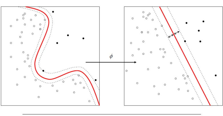
In addition to the linear soft-margin SVM, non-linear SVM can also be used for the data that is not linearly separable ([Doucet et al.,2007]). In non-linear SVM, a linear decision boundary is created by projecting the data through a non-linear functionφto a space with a high dimension. This means that data points which can not be separated by a straight line in their original spaceI are lifted to a feature spaceF where there can be a straight hyperplane that separates the data points of one class from an other. When projecting that hyperplane back to the input spaceI, it would have the form of a non-linear curve, as is shown in Figure

FIGURE3.2: The decision boundary in the non-linear SVM

min

w,b,εi

kwk2 2 +C

Pn

i=1εi

subject toyi(wTφ(xi) +b)≥1−εi,andεi ≥0,for alli.

wherewis the weight vector,C is the regularization constant which can be used to determine the trade-off between maximizing the margin and the number of training data points within the margin, and the mapping functionφprojects the training data into a suitable feature spaceF so as to allow for nonlinear decision surfaces. The non-linear SVM decision rule is simply to replace thex vectors in Equation 3.2with functionφ(x),

f(x) =sign

n

X

i=1

αiyiφ(xi)·φ(x) +b

!

(3.3)

The functionK(x, xi) = φ(x)Tφ(xi) is known as the kernel function. Since the

outcome of the decision function only relies on the dot-product of the vectors in the feature spaceF, it is not necessary to perform an explicit projection to that space. As long as a functionKhas the same results, it can be used instead. This is known as the kernel trick. So, the decision rule in Equation 3.3can be modified as

f(x) =sign

n

X

i=1

αiyiK(x, xi) +b

!

(3.4)

Popular choices for the kernel function are the Gaussian Radial Base Function

K(xi, x) =exp(−

and the polynomial kernel

K(xi, x) = (xi·x+c)d

It is important to notice that there is no such criterion that can be used to deter-mine which kernel is the best one. The kernel function selection is usually based on empirical practice and the comparison of prediction accuracy of SVM models using different kernels.

3.1.2 Multi-Class SVM

Originally, support vector machine (SVM) was designed for binary classification. However, the discrimination for more than two categories is often required in the real-world problems. Therefore, the multi-class pattern recognition has many ap-plications such as intrusion detection, speech recognition, and bioinformatics. The multi-category classification problems are usually divided into a series of binary problems so that the binary SVM can be directly applied ([Mathur and Foody,

2008]). Two representative methods are one-versus-rest and one-versus-one ap-proaches. Another methods are to directly deal with the multi-class problem in one single optimization processing such as the one by Crammer and Singer ([Duan and Keerthi,2005]). This kind of method combines multiple binary-class optimization problems into one single objective function and simultaneously achieves classification of multiple classes.

One-versus-rest method is probably the earliest used approach for muti-class SVM classification. It constructs k separate binary classifiers where k is the number of classes. The m-th binary classifier is trained using the data from the m-th class as positive examples and the remainingk−1classes as negative examples. Mathematically, givenn training data(xi, yi), wherexi ∈ Rp, i = 1,2, ..., n and

yi ∈ {1,2, ..., k}is the class ofxi, them-th SVM model solves the following

opti-mization problem

min

wm_,bm_,ξm

1 2(w

m₎T_wm_+CPn

i=1ξim

subject to:

(wm)Tφ(xi) +bm≥1−ξim,ifyi =m, (wm)Tφ(xi) +bm ≤ −1 +ξim,ifyi6=m,

ξ_im≥0, i= 1,2, ..., n

where the training dataxiare mapped to a higher dimensional space by the

determined by the decision function that gives the largest value. This decision rule can be written as

f(x) = argmax

m=1,2,...,k

(wm)Tφ(x) +bm

(3.5)

The disadvantage of the one-versus-rest approach is the imbalanced training data set. If all classes have an equal size of training samples, then the ratio of positive to negative samples in each individual classifier is_k−1₁. So, in this case, the symmetry of the original problem is lost.

Another classical method for multi-class SVM is the one-versus-one approach. This method buildsk(k−1)/2classifiers where each one is trained based on the data from two classes. For the training data from theith and thejth classes, the optimization problem is given by

min

wij_,bij_,ξij

1 2(w

ij₎T_wij _+CPT

t=1ξ ij t

subject to:

(wij)Tφ(xt) +bij ≥1−ξijt ,ifyt=i, (wij₎T_φ(x

t) +bij ≤ −1 +ξtij,ifyt=j,

ξij_t ≥0

After all k(k−1)/2 classifiers are constructed, the future testing is performed through voting strategy. Applying each classifier to a test sample would give one vote to the winning class and this test sample would be labeled to the class with the most votes. The number of classifier built by the one-versus-one method is much larger than the one-versus-rest method. However, the training speed of one-versus-one is much faster than one-versus-rest due to the reason that the size of quadratic programming in one is smaller than that of one-versus-rest.

Instead of creating several binary classifiers, a more natural way is to distinguish all classes in one single optimization processing, as proposed by Crammer and Singer. For ak-class problem, this method designs a single objective function for training allk-binary SVMs simultaneously and maximize the margins from each class to the remaining ones. The Crammer and Singer’s multi-class SVM method is performed by solving the following optimization problem:

min

wm,ξi

1 2

PK

m=1wTmwm+CPn_i=1ξi

suject tow_yT_iϕ(xi)−wtTϕ(xi)≥1−δyi,t−ξi i= 1,2, ..., n, t∈ {1,2, ..., K}

(3.6)

whereδi,j is the Kronecker delta, defined as 1 for i = j and as 0 otherwise. The

resulting decision function can be written as

argmaxmfm(x) =argmaxmwTmϕ(x) (3.7)

Note that the constraintsξi ≥0, i= 1,2, ..., n,are implicitly indicated in the

mar-gin constraints of Equation 3.6 whentequalsyi. The disadvantage of Crammer

and Singer’s method is the large computational complexity caused by the size of the resulting Quadratic Programming (QP) problem.

3.2

Gaussian Mixture Model

A gaussian mixture model is a weighted sum ofM component gaussian density functions which can be written as

p(~x|λ) = M

X

i=1

wig(~x|~µi,Σi) (3.8)

where~xis a D-dimensional data vector with continuous values,wi, i= 1,2, ..., M,

are the mixture weights which satisfy the constraint thatPM

i=1wi = 1, andg(~x|~µi,Σi), i= 1,2, ..., M, are the component gaussian density functions which can be written as

g(~x|~µi,Σi) =

1 (2π)D/2_|Σ

i|1/2

exp

−1

2(~x−~µi)

0

Σ−_i 1(~x−~µi)

(3.9)

Here,~µiis the mean vector andΣi is the variance-covariance matrix. A gaussian

λ={wi, ~µi,Σi}, i= 1,2, ..., M

The parameters in these components can be shared or tied, such as having a com-mon variance-covariance matrix. Moreover, the covariance matrices,Σi, can be

full rank or constrained to be diagonal. The choice of model configuration, such as number of components, full or diagonal covariance matrices and parameter shar-ing, is normally determined by the amount of data that is available to estimate the GMM parameters and how the GMM can be used in a particular biometric application.

Gaussian mixture model is the pattern recognition classifier most widely used in speaker recognition system due to its capability of representing a large class of sample distribution ([Huang et al., 2005]). One of the distinct properties of GMM is its ability to form smooth approximations to arbitrarily shaped densi-ties. The uni-modal gaussian model represents feature distributions by a position (mean vector), a elliptic shape (covariance matrix) and a vector quantizer (VQ). The nearest neighbor model represents feature distributions by a discrete set of characteristic templates. However, GMM represents these feature distributions in the way of acting as a hybrid between these two models by using a discrete set of gaussian functions, each with their own mean and covariance matrix, to allow a better modeling capability ([Reynolds, Quatieri, and Dunn,2000]). These three distribution models are compared in Figure 3.3. Plot(a) shows the histogram of a single feature variable extracted from a sample audio track, plot(b) shows the dis-tribution of this feature variable using uni-modal gaussian model, plot(c) shows shows a GMM and its ten underlying component densities, plot(d) shows a his-togram of the data assigned to the VQ centrod locations of a 10 element codebook. In a word, GMM not only provides a smooth overall distribution fit but also its components clearly detail the multi-modal nature of the density. The main at-traction of the GMM arises from its ability to provide smooth approximations to arbitrarily-shaped densities of long-term spectrum that are considered to be re-lated to the characteristics of the singer’s voice rather than the specific lyrics or tune.

There are several techniques available for estimating the parameters of a GMM, and the most popular and well-established method is maximum likelihood (ML) estimation. ML estimation aims to find such model parameters that the likelihood of the GMM can be maximized. Suppose we have a sequence ofN training feature vectorsX={~x1, ..., ~xN}, then the GMM likelihood can be written as

p(X|λ) = N

Y

i=1

FIGURE3.3: Comparison of distribution modeling

However, there is no closed-form solution to the maximization of the likelihood function in this case, because of its nonlinearity. Fortunately, the estimates of ML parameter can be acquired iteratively using the expectation-maximization (EM) algorithm due to the reason that it is rather straightforward to perform maximiza-tion even though it is non-linear funcmaximiza-tion. The basic idea of the EM algorithm is to estimate a new modelλ¯ using an initial model λso thatp(X|λ¯) ≥ p(X|λ)

([(McLachlan and Krishnan, 2007)]). The new model λ¯ then becomes the initial model for the next iteration and the process is repeated until some convergence threshold is reached. The initial model is typically derived by using some form of vector quantization (VQ) estimation, such asK-means clustering.

3.2.1 K-means Clustering

K-means clustering is a method of vector quantization and has been widely used for cluster analysis in data mining ([Wagstaff et al.,2001]). It aims to partition n

observations intokclusters in which each observation belongs to the cluster with the nearest mean. Mathematically, given a set of observationsXn×p={~x1, ..., ~xn},

is to divide these n observation intok clusters, S = {S1, S2, ..., Sk}, so that the

within-cluster sum of squares (WCSS) can be minimized. Here, WCSS is the sum of distance functions of each point in the cluster to thekcenters. The optimization problem ofk-means clustering can be written as

argmin S k X i=1 X

~x∈Si

k~x−µik2

whereµiis the mean vector in clusterSi. There are three steps ink-means

cluster-ing as shown below:

• Step1: Initialization

• Step2: Assignment

• Step3: Update

The first step aims to set up the k initial means. Commonly used initialization methods are Forgy and Random Partition. The Forgy method randomly chooses

kobservations from the data set and uses these as the initial means. The Random Partition method first randomly assigns a cluster to each observation and the ini-tial mean is the mean calculated from each cluster. The Forgy method tends to spread the initial means out, while Random Partition places all of them close to the center of the data set. Random Partition method is generally preferable for algorithms such as thek-harmonic means and fuzzyk-means. For the expectation maximization and standardk-means algorithms, the Forgy method of initializa-tion is preferable.

The second step is to assign each observation to the cluster whose mean yields the least within-cluster sum of squares (WCSS). Since the sum of the squares is the squared Euclidean distance, this is intuitively the nearest mean. This process can be given by the equation

S_i(t)=

xp:

xp−m

(t) i 2 ≤

xp−m

(t) j

2

∀j,1≤j≤k

(3.11)

where eachxp is assigned to exactly oneSt, even if it could be assigned to two or

more of them.

optimum, and the result may depend on the initial clusters. Figure 3.4shows this algorithm visually.

FIGURE3.4: Demonstration of K-means clustering

3.2.2 EM Algorithm

The EM algorithm can be started by either initializing the algorithm with a set of initial parameters and then conducting an E step, or by starting with a set of initial weights and then doing a first M step. The initial parameters, such as weights, mean vectors and covariance matrices, can be chosen in two ways. The first way is to select K random data points as initial means and use the covariance matrix of the whole data set for each of the initial K covariance matrices. The second way is to use some heuristic method, such ask-means clustering algorithm which can cluster the data first and then define weights based on k-means memberships. Mathematically, suppose that we have a data setD = {~x1, ..., ~xn}, where~xi is a

d-dimensional vector. Assume that all the points are generated in an IID fashion from an underlying densityp(~x). Here,p(~x)is defined as a finite mixture model withKcomponents

p(~x|Θ) = K

X

k=1

αkpk(~x|zk, θk) (3.12)

wherepk(~x|zk, θk are mixture components,1≤k≤K. z = (z1, ..., zK)is a vector

ofK binary indicator variables that are mutually exclusive and exhaustive. The

αkis the mixture weights, representing the probability that a randomly selected~x

was generated by componentk, wherePK

k=1αk = 1. The complete set of

param-eters for a mixture model withKcomponents is

Θ ={α1, ..., αK, θ1, ..., θK}

Given parameterΘ, the membership weight of data point~xi in cluster kcan be

written as

wik =p(zik = 1|~xi,Θ) =

pk(~x|zk, θk)·αk

PK

m=1pm(~xi|zm, θm)·αm

(3.13)

Here, the membership weights shown above are the probabilities that reflect the uncertainty, given~xi andΘ, about which of theK components generated vector

~xi.

EM algorithm can be defined as follows. This algorithm is an iterative algorithm which starts from some initial estimate ofλ, and then proceeds to iteratively up-dateλuntil convergence is detected. Each iteration consists of an E-step and an M-step.

• E-step

Denote the current parameter values as Θ. Compute membership weights wik

componentsαk, 1 ≤ k ≤ K. Note that for each data point~xi, the membership

weights have the constraint thatPK

k=1wik = 1. So, this will leads to anN ×K

membership weight matrix, where each of the rows sum to 1.

• M-step

This step aims to use the membership weights obtained in E-step to calculate new parameter values. LetNk=PNi=1wik, the column sum of the membership weight

matrix. Then, the new mixture weights can be obtained through

αnew_k = Nk

N ,1≤k≤K. (3.14)

The new mean vector is calculated in a manner similar to how we could compute a standard empirical average, except that thei-th data vector~xi has a fractional

weightwik. The equation of new mean vector is given by

~ µnew_k =

1 Nk N X i=1

wik·~xi,1≤k≤K (3.15)

The new covariance matrix can be calculated by

Σnew_k =

1 Nk N X i=1

wik·(~xi−~µnewk )(~xi−~µnewk )t (3.16)

This equation is similar in form to how we would normally compute an empirical covariance matrix, except that the contribution of each data is weighted bywik.

Note that this is a matrix equation of dimensionalityD×Don each side.

The iteration process of EM algorithm will be stopped when the convergence is detected. Generally, convergence can be detected by computing the value of the log-likelihood. This log-likelihood is defined as follows

logl(Θ) = N

X

i=1

logp(~xi|Θ) = N X i=1 log K X k=1

αkpk(~xi|zk, θk)

!

(3.17)

Chapter 4

Singing Voice Detection and

Separation

This chapter introduces two singing voice pre-processing techniques: singing voice detection and singing voice separation. Generally, the region in a popular song can be classified into two different parts. The first part is known as the vocal seg-ment. This segment not only has the singer’s voice but also involves background music. So it is actually a mixture of singing voice and instrumental sound. The second part is called the non-vocal segment. This segment only involves back-ground music and is irrelevant to the singer identification. So, in order to improve the performance of singer identification system, this segment should be removed out from the music recording.

Section 4.1 introduces the technique of singing voice detection. This technique aims to extract out the vocal segment from a popular music recording. Two ap-proaches are discussed here. The first approach is known as double GMM and has been most widely used by other researchers for many years. However, this tradi-tional method is so time consuming that we have to build two separate Gaussian mixture models. And also, the detection accuracy of this method is not satisfying. In order to remedy these disadvantages, an approach known as single GMM is proposed here.

Likewise, the singing voice contained in a song can be considered as relatively sparse in nature. Both algorithms are performed in the mono-channel music and belong to the field of blind source separation.

4.1

Singing Voice Detection

The singing voice is one of the most important characteristics of music. With the immense and growing body of music data, information on the singing voice could be used as a valuable tool for the automatic analysis of song content in the field of music information retrieval and many other applications. As the first pre-processing step in Auto-SID system, the problem of singing voice detection can be stated as follows: for a given song, classify each segment as being of either the pure instrumental type (known as the non-vocal segment) or as a mixture of singing voice and background music (known as the vocal segment) ([Regnier and Peeters,2009]).

In addition to the double GMM and single GMM, there also exists some other singing voice detection methods. In ([Berenzweig and Ellis, 2001]), Berenzweig and Ellis used Posterior Probability Features (PPF) obtained from the acoustic classifier of a general-purpose speech recognizer to derive a variety of statistics and models which allowed them to train a vocal detection system. In ([Chou and Gu,2001]), Chou and Gu have proposed a technique using a combination of har-monic coefficient based features, conventional Mel-frequency Cepstral Coefficient (MFCC) and log energy features in a GMM-based Speech/Music Discriminator (SMD) system to detect the singing voice. Kim and Whitman ([Kim and Whit-man, 2002]) have proposed a technique to detect the singing voice based on an analysis of the energy within the frequencies bounded by the range of vocal en-ergy. This has been achieved using a combination of an IIR filter and an inverse comb filter bank.

4.1.1 Traditional Method - Double GMM

Music recordings have got both vocal and non-vocal regions within it. Here, the non-vocal regions are those regions of the music recordings having no voice con-tents within them. As far as singer identification is concerned, the non-vocal re-gions are irrelevant. The singing voice detection is performed in order to find and reject the non-vocal regions in a music recording. For that purpose, a stochastic recognizer needs to be built to differentiate between vocal and non-vocal segments in the music recording.

The block diagram of this process is given in Figure 4.1. In the training phase, two audio tracks are collected from internet database. The first audio track involves vocal-only music and is denoted as vocal track. The second audio track contains instrumental-only music and is known as non-vocal track. The features of these two audio tracks are extracted out through MFCC and further used for training two separate Gaussian mixture models, the vocal GMM (λV) and the non-vocal GMM (λN). The parameters of the Gaussian mixture model like mixture weights, covariance matrices and mean vectors are initialized by k-means clustering algo-rithm and modified by expectation-maximization (EM) algoalgo-rithm.

FIGURE4.1: The block diagram of double GMM

In the testing phase, the music recording is firstly decomposed into a set of seg-ments of one second length. Then for each segment, its MFCC feature matrix is calculated and the column mean of this matrix is input into the vocal and non-vocal GMMs for log-likelihood value calculation. Finally, the segment type is de-termined by these values and the decision rule can be given by the equation

K=logP(~xmean|λV)−logP(~xmean|λN)

K >0,vocal segment.

K ≤0,non-vocal segment.

The vocal segments will be saved for further analysis while the non-vocal seg-ments have to be discarded.

4.1.2 Improved Method - Single GMM

Although the double GMM discussed above has been widely used, some defects exist within this method. First, double GMM is very time consuming due to the reason that two Gaussian mixture models have to be built. Second, the vocal GMM (λV) is trained by using the features extracted from the vocal track which is actually a mixture of singing voice and background music. As a result, the vocal GMM is so sensitive to the background music that the detection accuracy has been seriously affected.

In order to remedy these disadvantages, another approach known as single GMM is proposed in this thesis. The block diagram of single GMM is given in Figure

4.2. As with double GMM, the recognizer in single GMM also has two phases: training and testing. However, instead of building two Gaussian mixture models, the single GMM only has to train the non-vocal one (λN) and the decision rule for determining the segment type is also changed. The reason why only non-vocal GMM be trained is that the data used in this model is actually pure instrumental sound. Since the log-likelihood values calculated in the testing phase can be re-garded as a similarity measurement between two audio signals, then the segment with the smallest log-likelihood value tends to have the largest ratio of singing voice to background music.

According to this fact, the segment type can be determined by ranking strategy and the decision rule can be given by the following equation:

Ki=logP(~xi|λN),1≤i≤M ∈K~

Select 10 segments

which have smallest values amongK~

(4.2)

Here,M is the number of segments.

4.2

Singing Voice Separation

The vocal segment obtained from previous step is actually a mixture of singing voice and background music. Since the data used for singer identification is ac-tually extracted from singer’s voice, then the instrumental sound should be re-garded as noise and we need to find a way to segregate the singing voice from background music. This segregation process is know as singing voice separation and it has many applications in real world such as lyrics recognition and align-ment, singer identification and music information retrieval.

The singing voice separation is a very challenging problem due to the fact that it is very difficult to determine the relationship between the number of observed signals and that of sources ([Huang et al.,2012]). Moreover, we must also need to confirm the type of sources in the mixed music recordings. Although both the singing voice and the speaking sound are produced by vocal tract, the speech separation techniques can not be directly used for singing voice separation. This is mainly caused by the interfering sounds like background music. In a real acoustic environment, the music accompaniment is correlated with the singing voice but uncorrelated with the speech ([Hsu and Jang,2010]). As a result, it is extremely hard for us to segregate the singing voice from accompaniment.

4.2.1 Non-negative Matrix Factorization

Non-negative matrix factorization (NMF), also know as non-negative matrix ap-proximation, is an algorithm for multivariate data analysis where a matrixVn×mis

factorized into the product of two matricesWn×randHr×mas shown in Equation

4.3, with the property that all of the three matrices have no negative elements. Because of this non-negative property, the resulting matrices become easier to in-spect.

V ≈W H (4.3)

Specifically, suppose that we have a set ofp-dimensional vectors, and these vectors construct a matrixV ofp×nsize wherepis the number of variables andnis the number of examples. This matrix is then approximately decomposed into a matrix

W ofp×rsize and a matrixH ofr×nsize. Normally,r is chosen to be smaller thannorpso thatW andH are smaller than the original matrixV. This leads to a compressed version of the original data matrix.

In order to findW andH, two cost functions have been proposed so that the qual-ity of the approximation can be quantified. The first cost function is constructed using the square of the Euclidean distance betweenV andW H as shown in Equa-tion 4.4.

kV −W Hk2 =X ij

(Vij −(W H)ij)2 (4.4)

This is lower bounded by zero, and clearly vanishes if and only ifV =W H. An-other cost function is based on the divergence ofV andW Has shown in Equation

4.5.

D(V||W H) =X ij

Vijlog

Vij (W H)ij

−Vij+ (W H)ij

(4.5)

Like the first cost function, this cost function is also lower bounded by zero, and vanishes if and only ifA = B. It reduces to the Kullback-Leibler divergence, or relative entropy, whenP

ij

Vij =P ij

(W H)ij = 1, so thatV andW H can be regarded

as normalized probability distributions. Therefore, the optimization problem can be written as

Problem 1:Minimize kV −W Hk2 with respect toW andH,

Problem 2: MinimizeD(V||W H)with respect toW andH,

subject to the contraintsW, H ≥0

These two optimization problems can be solved by multiplicative update rules which are demonstrated as follows.

Theorem 1: The Euclidean distancekV −W Hk is non-increasing under the up-date rules

Haµ←Haµ (W

T_V) aµ

(WT_{W H)} aµ

Wia←Wia (V H

T₎ ia

(W HHT₎ ia

(4.6)

The Euclidean distance is invariant under these updates if and only ifW andH

are at a stationary point of the distance.

Theorem 2:The divergenceD(V||W H)is non-increasing under the update rules

Haµ ←Haµ

P

iWiaViµ/(W H)iµ

P

kWka

Wia ←Wia

P

µHaµViµ/(W H)iµ

P

vHav

(4.7)

The divergence is invariant under these updates if and only ifW andH are at a stationary point of the divergence.

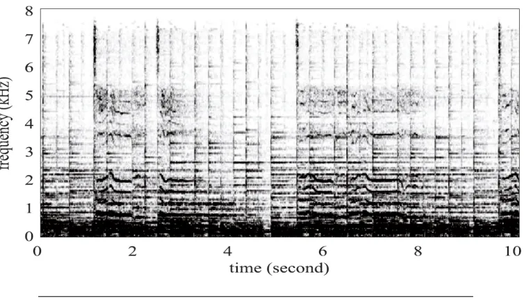
For a vocal segment obtained from singing voice detection step, its spectrum can be regarded as an input matrixV of NMF, as is showed in Figure 4.3. The non-negative value at any position(f, t)in matrixV is the amplitude of the signal at frequency-binf and framet. Here, suppose that the matrixV hasT columns and

Frows. After a decomposition using NMF, we will obtain a matrixW containing

Rbasis vectors of lengthFand a matrixHcontaining the coefficients of each basis vector along the time axis ([Helen and Virtanen,2005]).

The resulting matrices become sparse due to the non-negative constraint. As a result, we can conclude that each basis vector contains the frequencies that are produced simultaneously. For the music accompaniment, the simultaneous fre-quencies can be regarded as timbres or harmonics of each note. So, the value of

FIGURE 4.3: Spectrum of a music clips as an input matrix V of NMF, where dark color represents high amplitude and vice versa

view of these facts, for singing voice separation, the basis vectors of instrumental sound are detected and removed, instead of that of the singing voice.

The singing voice separation using NMF has three steps. The input music sig-nal is firstly transformed from time domain to frequency domain so that it can be factorized by NMF. Then, NMF is performed before the component selection. If the selected components contain the frequencies extracted from the music accom-paniment, we should use some filters in the refinement stage to eliminate them. Finally, the singing voice is reconstructed. The details of these steps are showed as follows.

• Step 1: Pre-processing and Decomposition

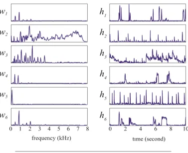
Firstly, the mono-channel music recording is downsampled at the sampling rate of 16,000 Hz. Then it is transformed from time domain to frequency domain using Discrete Fourier Transform (DCT) with the Hamming window of 32 ms frame size and 16 ms overlapping. Then, the NMF input can be initialized by the magnitude or amplitude of the spectrum. In addition, the number of basis componentsR is initialized to 64. The resulting matricesW andH can be obtained through the NMF of the input matrixV. The basis vectors ofW and the coefficients inHalong the time axis are showed in Figure 4.4.

• Step 2: Component Selection

FIGURE4.4: An example of components decomposed by NMF into matrices W (left) and H (right)

decomposed by NMF might not separate each note of each instrumental sound correctly. However, these instruments except for percussion tend to be played continuously in time. On the basis of these ideas, the coefficients in matrixHare considered as the tool which can be used to show us how each component varies along the time axis. For example, all the graphs in the right column of Figure

4.4 are the coefficients of basis components in the left column. We can see that

h2 andh5are rhythmic which means that the sound of this component is played

rhythmically. Therefore, these two components should be eliminated. Normally, the singing voice produced by human does not last for a long period. According to this, if the basis spectrum of a music clip lasts too long, then it is most likely that this spectrum is not from the singing voice. For example, in Figure 4.4,h3 is

obviously a continuous event and therefore it should be removed.

• Step 3: Signal Reconstruction

and lack of phase information. In order to fix this, the new spectrum is calculated in the way that the complex value in any position is the product of each individual element in this matrix and the original spectrum in the same position.

FIGURE 4.5: The spectrogram of WH after component selection, where dark color represents high amplitude and vice versa

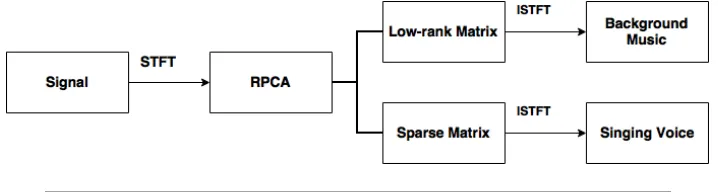
4.2.2 Robust Principal Component Analysis

Robust Principal Component Analysis (RPCA