Faculty of Engineering and Surveying
Validation of the Sydnet, Continuously Operating Reference
Stations for use in Global Navigation Satellite System surveying
A dissertation submitted by
Mr. Jamie Richard Black
In fulfilment of the requirements of
Bachelor of Spatial Science (Surveying)
Contents
Section Page
1.
Introduction
1
1.1 Problem Statement 1
1.2 Project Aim 1
1.3 Project Background 3
1.4 Research Justification 6
1.5 Summary 7
2.
Literature Review
8
2.1 Introduction 8
2.2 GNSS Overview 8
2.2.1 Static GNSS Surveying 8
2.2.2 Real Time Kinematic Surveying 9
2.2.3 Continuously Operating Reference Stations (CORS) and Networks 10
2.3 Operational CORS Networks 13
2.3.1 Sydnet 13
2.3.2 SunPOZ 16
2.3.3 MELBpos 17
2.4 Sydnet testing to date 18
2.5 Standards, Legislation and Directions 20
2.6 Summary 21
3.
Research Method
22
3.1 Introduction 22
3.2 Planning the Control Network 22
3.2.1 Two dimensional class and order of network control marks 24
3.2.2 Height class and order of network control marks 24
3.3 Resources 25
3.3.1 Personnel 25
3.3.2 Equipment 25
3.3.3 Software 27
3.4 Field Test Technique 28
3.4.1 Fast Static 28
3.4.2 RTK Static 30
3.5 Data Processing 32
3.5.1 Acquisition of Sydnet data 32
3.5.2 Leica Geo Office (LGO) 34
3.5.3 Data and Error Analysis 34
3.5.4 Conformity to NSW legislation 35
3.6 Conclusion 35
4.
Results
36
4.1 Introduction 36
4.2 Leica Geo Office Processing 36
4.3 Accuracy 38
4.3.1 Horizontal Accuracy 39
4.3.2 Vertical Accuracy 44
4.4 Precision 51
4.5 Reliability 59
5.
Analysis
61
5.1 Introduction 61
5.2 Horizontal Accuracy 61
5.2.1 Static Observations 62
5.2.2 RTK Observations 66
5.3 Height Accuracy 67
5.3.1 Static Observations 68
5.3.2 RTK Observations 70
5.4 Precision 71
5.5 Reliability 73
5.6 Conclusion 74
6.
Conclusion
76
6.1 Introduction 76
6.2 Conclusions 76
6.2.1 Horizontal Accuracy 76
6.2.2 Vertical Accuracy 76
6.2.3 Precision 77
6.2.4 Reliability 77
6.3 Recommendations 77
6.4 Final Remark 79
7.
References
80
8.
Appendices
82
List of
Figures
Page
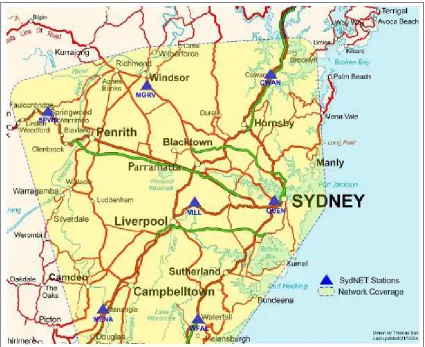
1.1 Sydnet Configuration – Sydney basin only 4
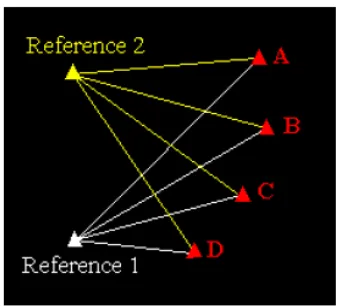
2.1 Rapid Static Baselines 9
2.2 VRS field set-up procedure 11
2.3 Leica Spider 12
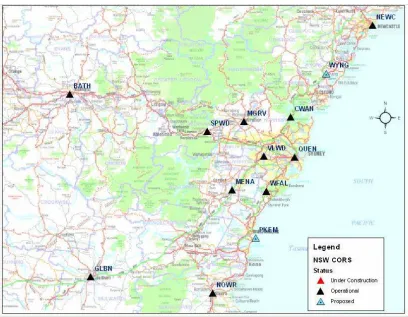
2.4 CORS locations over NSW
14
2.5 SunPOZ CORS network 16
2.6 MELBpos CORS network 17
3.1 Location of SCIMS Network Control Marks 23
3.2 SCIMS State Survey Mark (SSM) 108024 29
3.3 RTK observation as TS 1582 ‘COOK’ 30
3.4 RTK observation at SSM 108024 31
3.5 Post processing data acquisition website 33
4.1 Chippendale CORS satellite window 15/07/2008 38
4.2 Average two-dimensional static observed coordinates and respective σ 40 4.3 Individual static baseline calculations to PM 52389 and respective σ 41 4.4 Average two-dimensional RTK observed coordinates and respective σ 42 4.5 Average RTK single baseline solutions over two separate observations 43 4.6 Average static observations & average RTK observations compared to SCIMS
MGA values of network control marks 44
4.7 Average static height observations and respective σ 46
4.8 Individual baseline height observations 47
4.9 Average RTK observed heights and respective σ 48
4.10 Individual RTK height observations to all network control marks 49 4.11 Average static observations & average RTK observations compared to SCIMS
AHD71 values of network control marks 51
4.12 95% confidence interval of average static observations 52 4.13
Day to day comparison of static observations and standard deviation of data sets 53 4.14 95%Confidence Interval of average RTK observations (Excluding PM 52389) 54 4.15
Day to day comparison of RTK observations and standard deviation of data sets 55 4.16 %Confidence Interval of average static heights
56 4.17 Comparison of heights from day to day static observations and standard
deviations of data sets 57
4.18 95%Confidence Interval of average RTK heights (excluding PM 52389)
58 4.19 Comparison of heights from day to day RTK observations and standard
5.1 TS 2888 ‘Long Reef’ 63
5.2 Large pine causing possible obstruction at SSM 24639 65
5.3 Overhanging trees virtually covering the available sky at TS 1582 ‘COOK’ 65
5.4 SSM 108024 and possible multipath object to the west 67
List of
Tables
Page
3.1 Control Network Class and Order 23
3.2 Static observation instruments and accessories 26
3.3 RTK observation instruments 27
5.1 Variance of static observations to TS 2888 62
5.2 Individual static baseline observations to TS 2888 63
Abstract
Permanent Global Navigation Satellite System (GNSS) networks of Continuously Operating Reference Stations (CORS) are becoming routinely used for surveying activities, including maintenance of the geodetic datum, deformation monitoring and land surveying. These networks consist of several fixed GNSS antennas and receivers that operate on a 24-hour basis and provide positional information to those who request it. Before a network can be used in survey application it must be validated to ensure the results required for specific tasks are achievable.
The NSW Department of Lands (DOL) has developed a network of CORS, predominantly covering the Sydney basin called Sydnet. The network objective was to provide a user with centimetre accurate coordinates, regardless of their position, using static and real-time kinetic (RTK) applications. This dissertation tested and validated the coordinate information provided by Sydnet against class 2A and class B for horizontal and class LB and class LC for AHD heights of coordinated permanent survey marks found in the northern suburbs and northern beaches of Sydney. The outcome determined whether the information provided could position a user with an accuracy and precision that is acceptable under current legislation.
The aim was to evaluate and critically analyse the horizontal and vertical results of GNSS observations using Sydnet with respect to accuracy, precision and reliability.
Research into the Sydnet system was critical to determine its functionality and limitations before, a network of control marks was planned to test these limits. The test network was based on careful planning to ensure that the special selection of known coordinated survey marks chosen, provided the necessary geometry along with mocking field simulated situations i.e. sky obstructions. The essential field observation data was collected in a manner that conformed to the ICSM SP1 standard to make certain the best possible outcome for tests 1 and 2 were achieved which were as follows:
Test 1: Rapid static GNSS observations undertaken were to comply with a Class B survey requiring
two occupations of seven of the eight marks in the network and three occupations of the eighth mark all for a half hour period.
Test 2: Real-time static application occupied each mark in the network firstly, for a ten minute period
from two separate base CORS and secondly, for a one minute period from the same two base CORS on a separate day.
Through Leica Geo Office and Microsoft Excel software, the data was processed to determine observed values at each network control mark, and then compared with the true value of each mark, with the final outcome determining Sydnet’s accuracy, precision and reliability.
Candidates Certification
I certify that the ideas, designs and experimental work, results, analysis and conclusions set out in this dissertation are entirely my own efforts, except where otherwise indicated and
acknowledged.
I further certify that the work is original and has not been previously submitted for assessment in any other course or institution, except where specifically stated.
Your Full Name Jamie Richard Black
Student Number: 50032304
Acknowledgments
This research was carried out under the principal supervision of Mr Glenn Campbell and Mr Peter Gibbings of the University of Southern Queensland whom have provided great advice and guidance throughout.
Simon McElroy of the NSW Department of Lands has provided a great deal of assistance in the generation of this paper. His knowledge and skills in this field have been of benefit to the learning process. He has guided me from the beginning with enthusiasm and kindness.
My employer Connell Wagner (CW) has been the funding machine behind this project and I would especially like to thank CW’s NSW survey discipline leader Graham Tweedie for allowing me many hours to research, use the necessary equipment and analyse the captured data.
1.
Introduction
1.1
Problem Statement
Continuously Operating Reference Station (CORS) networks are becoming a common means of conducting GNSS observations throughout the world. CORS networks are found in many countries and cities and are used for applications like geodetic and tectonic plate monitoring, machine guidance and land surveying.
Sydnet is one such CORS network that offers both static and real time kinematic (RTK) operations throughout the Sydney region in the state of New South Wales, Australia. Although the system has been implemented since 2002 (Kinlyside, 2006), the RTK component of Sydnet has only become available to users since May 2008 (DoL, 2008).
Survey firms now have the opportunity to use Sydnet for static and real time observations in survey applications. Prior to use in project applications that will go to clients with an expectation of correctness, Sydnet must be validated by each firm to ensure their knowledge of the system and its limitations.
1.2
Project Aim
Task 1: Research the background into the development of the Sydnet CORS system
It was essential to this project that the development of the Sydnet system was understood to determine its purpose and functionality.
Task 2: Plan a control network of permanent survey marks for use in the validation application
A significant part of the validation process involved a planned network of Survey Control Information Management System (SCIMS) permanent survey marks that had sufficient class and order in both horizontal and vertical manners. It was important to maintain good geometry and use a diverse selection of marks that have been coordinated using different methods
o i.e. EDM traversing and GPS observations.
Task 3: Identify and select a methodology to complete a validation of the GNSS network
There were many methods that can be used to locate the marks chosen in the GNSS network. Some methods are better than others and it was important to determine the ‘best’ method to ensure a minimisation of errors. In order to achieve this, the Intergovernmental Committee on Survey and Mapping (ICSM), Standards and Practices for Control Surveys (SP1) was researched and adopted.
Task 4: Become familiar with the instrumentation
Task 5: Analyse and evaluate field data
This objective ties in heavily with the aim of the project and was the core to the validation of the Sydnet system. The data received from the SV’s was processed using Leica Geo Office to determine the accuracy and precision of data delivered by each adopted CORS base.
Static measurements at each survey mark were post processed with respect to the four nearest CORS.
RTK measurements involve the adoption of a single reference station at a time due to network limitations currently offering single base only.
The results will then be analysed to determine the differences between static and RTK solutions when compared to the specific survey mark occupied. All coordinates are on MGA.
The results of the analysis will then be evaluated to determine the ‘useability’ of Sydnet in survey projects by comparison against legislative requirements and/or specific project limitations.
1.3
Project Background
Figure 1.1: Sydnet Configuration – Sydney basin only (Rizos et al., 2004)
Global Positioning Systems (GPS), more recently called Global Navigation Satellite Systems (GNSS), have been evolving at a rapid rate since the early 1970’s. Since the initial development by the United States of America (USA) government for military use, many changes have come about to allow the general public access to GNSS. Surveyors have taken advantage of the availability of the system and in doing so have developed an advanced method of taking measurements of the earth.
GNSS applications range from standard modes of differential GNSS, using pseudo-range techniques to precise carrier phase measurements, using ambiguity-solving algorithms. Pseudo-range GNSS can provide solutions up to 0.25 of a metre but is generally accepted as metre accurate (Leica
There are limits that exist for conventional differential GPS that restrict the length of survey baselines to approximately 10 - 20km (Gibbings et al., 2005) before atmospheric differences can distort the signals received, making the ambiguity-solving component difficult to impossible. Corrections can be calculated and applied to post processed surveys however RTK surveys cannot be updated with corrections in the field, unless a post processing adjustment has occurred.
The development of CORS networks has once again revolutionised GNSS technology. Currently used in many cities and countries around the world, CORS networks are rapidly becoming ‘the more sensible approach’ to GNSS surveying. A common practice for CORS networks is to adopt a Virtual Reference Station (VRS), allowing corrections to be processed by more than one CORS and providing a virtual base station in the local area to be surveyed. Using this method can provide for results of centimetre to sub-centimetre accuracies.
The NSW DOL has in place a network of CORS, however at this stage has not yet decided upon the application of network RTK, hence at present, only single base RTK is available from certain sites in the Sydney basin and nearby rural areas. Whether using a VRS or single base RTK, adopting a CORS as a base station not only eliminates theft possibilities by abolishing the need for a localised base station, but can also provide correction data for atmospheric bias over the survey baseline required regardless of the length (provided both CORS and user receiver can receive signals from the same series of satellites (SV’s) to solve phase ambiguities).
The surveying industry like many others is regulated by legislation on a State by State basis and with recent inclusions into the Surveying Regulation 2006 (NSW), determining specific accuracies of both Terrestrial Positioning Systems (TPS) and GNSS use, it is important that the CORS network provides results that enable surveyors to complete day to day surveys within the limits of the regulation. This topic has been chosen to determine whether or not the data provided by each CORS enables surveyors to achieve results that are within the set limits and if not, whether there are alternate methods to help provide compliance to the legislation.
1.4
Research Justification
Many firms around the world have more recently placed a strong focus on Quality Assurance as a way of verifying results or products prior to their release to clientele. The surveying industry lies within the list of firms that requires these measures; therefore it is becoming increasingly important to be able to understand how results have been derived in order to verify them. Validating Sydnet using known methods and standards provides an understanding hence the verification process is enabled.
As surveyors, we must know that the results we are observing are within specific accuracy and that we can have confidence in them. This is paramount to a successful survey firm, where results are often passed on to clients who expect correctness.
Confidence in results goes hand in hand with knowing the limits of a system. Sydnet, which is in its early stages of release for use, requires validation on the part of each user. This allows users to determine the limits in which they can apply the use of Sydnet in project application. At the same time the reliability of the system can be determined to provide the user with a reasonable idea of survey completion percentages using Sydnet in the field.
1.5
Summary
This research was expected to result in an analysis that determined whether Sydnet GNSS surveys comply with current NSW legislation and the needs of users. It is essential for survey firms to be able to rely on data provided by external sources e.g. DOL Sydnet system and obtain the best possible results by adopting good standards of practice like ICSM SP1, section B for GNSS surveys.
A review of literature for this research will identify the current acts and regulations in place to maintain quality standards across the NSW board. Current standards and practices will be reviewed to
2.
Literature Review
2.1
Introduction
With CORS systems in use all around the world, there is a certain need for review of current operation limitations, accuracy, precision and reliability testing. Many countries have adopted CORS systems for monitoring and surveying purposes and on Australia’s eastern sea board, CORS networks are in place in capital cities with the intention of expansion into state wide networks like GPSnet in Victoria. .
Throughout this chapter it is intended to firstly take a look into methods of conventional GNSS surveys to understand the limitations of their application; and secondly review current literature with respect to CORS networks located on the eastern sea board of Australia with particular interest in Sydnet’s prior accuracy, precision and reliability testing. Other CORS networks in Victoria and Queensland will also be investigated along with their current operations.
Standards and regulatory requirements must also be reviewed to understand what limitations can be placed upon observations from Sydnet, with a major objective of establishing whether the observations have the ability to comply. NSW Surveying Regulation 2006 is to be reviewed along with the Surveyor General’s Directions No.9, GPS Surveys, for this purpose. Standards exist that must be examined to ensure proper methods are applied to observations hence ICSM SP1 will also be reviewed.
2.2
GNSS Overview
2.2.1 Static GNSS Surveying
Good survey practice, as shown in Figure 2.1, requires the occupation of each station (shown A, B, C and D) twice from two separate receivers. This offers redundancy and an independent check on the original observations. This process does have limits as stated in the Department of Sustainability and Environment (DSE), Surveying Using Global Navigation Satellite Systems (2003), where it is indicated classic static methods (not shown here) and rapid static methods (see Figure 2.1) provide best results when the baselines are less than 10km and 5km respectively.
[image:20.595.248.419.424.577.2]Other limitations can be found in personnel resources and time management. To operate such a technique generally requires the use of at least two people but may require more dependent on the number of receivers. Effectively the time taken to complete the survey is double that of the required work with two occupations of each station. Time and personnel savings may be viable without the requirement of extra instrumentation when adopting permanent reference stations.
Figure 2.1: Rapid Static Baselines (DSE, 2003)
2.2.2 Real Time Kinematic Surveying
allows the comparison of a calculated position from the SV’s with the known position of the mark. The difference (or correction) can then be transmitted via radio link to the roving unit. The roving unit then uses its calculated position from the SV’s and then applies the correction data it is receiving from the base station by radio to determine an accurate position in real time.
This technique itself has revolutionised GPS surveys and the technicalities involved in the process are far beyond the scope of this project, however RTK does have many limitations. Solving the ambiguities for real time application involves the same parameters as static surveys requiring data from SV’s to reach both receivers. The essential feature of RTK surveys is the correctional data received from the base station. If radio contact cannot be made, correctional data cannot be received at the rover end, deeming the resultant position inadequate. Often distance and topography are the reasons for loss of radio contact. Typically low strength radio signals can range between 1 to 3 kilometres but can be dependant on topography i.e. generally areas with undulating terrain will have an adverse affect on radio contact ability.
2.2.3 Continuously Operating Reference Stations (CORS) and Networks
The concept of a Continuously Operating Reference Station is a 24-hour a day, 7 day a week operating base station that logs data available to those with authorised access. This data can be accessed for the period in which the surveyor requires and can be delivered by email in the desired format for application within the GNSS processing software. When placed strategically around a specific area (e.g. the Sydney basin) the received data from each CORS can be processed simultaneously and provide an operational network of base stations.
Although many of these systems operate throughout Australia, the methods used to determine the real time position of the user does vary.
Many networks use the Trimble Virtual Reference System (VRS) whereby multiple reference stations are used to obtain the best possible solution for a position in the local area. A virtual reference station is then created about that position with all corrections being supplied as though there was an existing base station present at that point (shown in Figure 2.2 below).
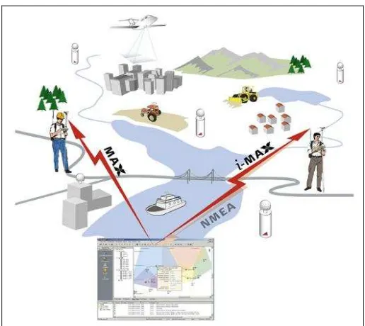
Figure 2.2: VRS field set-up procedure (Vollath et al., 2002)
Figure 2.3: Leica Spider (Source: Leica Geosystems, 2006a)
Yet another option and the most relevant to this project is the Raw Data Broadcasting. Different to a network solution system, this model provides users with a single base solution from an individual reference station. To eliminate the distant dependant errors, corrections are broadcast from a NCC and received by the user, where computations are performed to provide a solution (Rizos et al., 2003).
2.3
Operational CORS Networks
2.3.1 Sydnet
Background
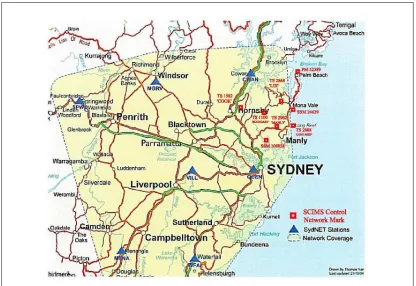
Figure 2.4: CORS locations over NSW (Source: DOL
<http://sydnet.lands.nsw.gov.au/images/MetroNETCoverage.jpg>)
Operations and Implementation
To promote the network it must be proven that conventional GNSS techniques are deficient and/or limited in providing results for specific applications. Rizos et al. (2003, 2004) outline the limits of the standard mode of precise differential GPS (DGPS) positioning and presents network RTK as the solution to these limits. Unfortunately, to operate a RTK network that covers a large area there are many complications that must be overcome. Perhaps one of the more crucial of these is the
Another crucial feature is the time taken to determine AR for RTK applications, measured in seconds. It is important that the locations of the base stations be spread appropriately to be able to model distant-dependant errors and enable accurate point positioning, rapidly solving AR, and thus enabling centimetre accurate real-time position.
Using standard DGPS, correction data is relayed via radio on a specific frequency from the base station to the receiver. Advancements in technology have now allowed real-time correction data to be transmitted by GSM mobile network or by wireless internet connection in the field. The hardware must have the capability to receive this data if a CORS network is to be utilised in RTK surveys. It must also be noted that mobile coverage plays an integral part in the ability to receive correctional data (i.e. No mobile coverage = No network RTK).
Users Ability
Static GNSS surveying methods are the same as conventional methods except for one major difference. This difference is removal of the need for a local base station. Using any particular base station (generally the closest) eliminates the requirement for a local base station effectively saving on time and cost of the survey.
Users must register to be able to gain access to the Sydnet Receiver INdependent Exchange (RINEX) data. Once registered, users are able to access Sydnet data from any particular base station, via the DOL website <http://sydnet.lands.nsw.gov.au/sydnet/login.jsp>. Upon receipt of the data, it can be uploaded into compatible software and used as a reference station.
Assuming that all users have their instruments configured correctly, the benefit and ease of use of the system is apparent. The process is really as simple as turning on the instrument, waiting for the automatically configured internet connection to occur, then simply choose the required base station and wait for initialisation (generally under 60 seconds).
2.3.2 SunPOZ
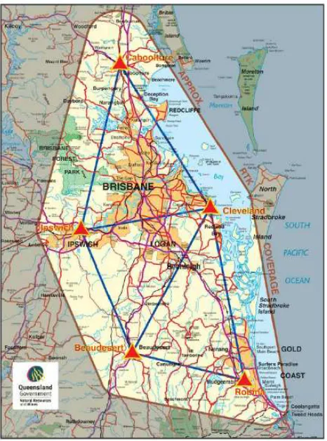
[image:27.595.218.451.430.744.2]The Queensland Department of Natural Resources and Water (NRW) have developed a CORS network that utilises the VRS system. Located in the states south-east in the metropolitan regions, SunPOZ is providing users with results comparable to, and in some respects superior to, classic RTK techniques. These results have determined that the SunPOZ system has achieved average accuracy to the order of 13mm in a two dimensional vector format with a 95% Confidence Interval (CI) of +/- 20mm. The accuracy of height average achieved a remarkable 5mm with a 95% CI of +/- 56mm (Gibbings et al., 2005).
2.3.3 MELBpos
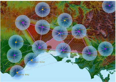
MELBpos has been developed to service the greater Melbourne regional area in the southern state of Victoria. Much like SunPOZ, Victoria Lands has opted for a VRS network solution for RTK application. Five stages of testing conducted in late 2005 and June 2006 consisted of:
i) Accuracy and precision testing ii) Daily repeatability
iii) Influence of inter receiver distance
iv) Comparison of data from different manufactures
v) Advantages and disadvantages of different format messages
[image:28.595.131.536.453.740.2]The results of over 160 hours of observed data produced results to determine the accuracy of easting, northing and ellipsoidal heights were 3mm, 4mm and 4mm respectively. Precision results were 4mm, 6mm and 10mm in easting, northing and ellipsoidal heights (Gordini et al., 2006)
2.4
Sydnet testing to date
The operational ‘go-ahead’ was given to Sydnet users on 1 May 2008 (see Appendix D). Prior to this date there has been testing conducted on the CORS network as a whole with mixed results. Roberts et al. (2007) have provided results of the primary testing of the Sydnet CORS network in its beta phase with mixed results over the Sydney basin.
It is an important factor to know how each CORS has been assigned its coordinates and AHD value. Through personal communication with a DOL Geodesy Senior Surveyor, Simon McElroy, it has been established that the two dimensional coordinates have been obtained by six sets of observations, each over a twenty-four hour period with the final position based on the ITRF2000 Cartesian coordinates (McElroy, 2006). Heights have been assigned to each CORS locally by simultaneously observing the original Australian National Levelling Network (LAL1) marks in the local areas of each reference station. Two sets of one-hour static observation periods was the method applied and processed with NGS antenna models and precise orbit data. Each CORS is tied to a minimum of 3 or 4 marks. In some cases where the original LAL1 marks have been destroyed or disturbed, checks have been performed on LBL2 marks (McElroy, personal communication, 2008).
Phipps has investigated the discrepancies found in AHD values of observed versus SCIMS
coordinated marks in the eastern and southern suburbs of Sydney. It was concluded that there were systematic biases in the values obtained from observations however further study is required to determine whether the differences in height are due to errors in AHD71 and the AUSGeoid98 model or errors in the Sydnet correction data. The conclusion to Phipps’ investigation outlines the relevance and need for testing in other regions of Sydney.
A discussion with a DOL Geodesy Senior Surveyor, Simon McElroy, has also provided evidence that discrepancies in Sydnet heights could be from several sources. He has indicated that not only are there uncertainties with Ausgeoid98 – Ellipsoid separation values in relation to the location of the reference stations but also errors associated with the general receiving of SV data. In several test sessions conducted in mid 2007, the range in RL varied by as much as 130mm and 175mm for baselines of 8km and 19km in length respectively when recording data as individual positions over the same mark at a 1 second epoch rate. It must be noted that the ranges include some severe
observation spikes and generally the ranges fell within 50mm. As time increased through the observation period, average results became more reliable due to the sample size increasing.
Aside from testing of accuracy and precision, the DOL has thoroughly tested and documented a receiver’s performance with respect to internet connection times, float solution times, fixed ambiguity times, ambiguity resolution success rate, ambiguity re-initialisation times and ambiguity initialisation success rate of many types of receivers (McElroy, 2007) hence any further study is not required.
2.5
Standards, Legislation and Directions
As previously discussed, there are standards required when conducting GNSS surveys. For the purposes of this project the Inter-Governmental Committee of Surveying and Mapping (ICSM),
Standards and Practices for Control Surveys (SP1) version 1.7, September 2007 has been adopted. In order to achieve the required results these standards must be followed.
The chosen network of survey marks has each been assigned a particular class and order under Part A, Section 2.2 of SP1. Survey Techniques, under Part B, Section 2, requires review for method clarity. Under sub-section 2.6 titled Global Positioning Systems (GPS) a complete run down of methods exist including: planning a GPS survey, requirements for GPS observations, specified observation
requirements for various GPS techniques, analysis of data and field note requirements.
The Surveying Regulation 2006 regulates legislative requirements for cadastral surveys in NSW. Significant changes have been made in the 2006 Regulation to accommodate for the increase of GNSS use in cadastral applications (previously called GPS surveys in 2001). An important change is the alteration of accuracy requirements. Under clause 25 (2) of the Surveying Regulation 2006, it is stated ‘In making a survey, a surveyor must measure all lengths to an accuracy of 10 mm + 15 parts per million (ppm) or better at a confidence interval of 67%’. An example would show that a baseline of 1km in length should provide coordinates to an accuracy of 25mm, being one standard deviation from the mean value of the observations. Like wise a 10km baseline provides expected accuracies of 160mm. Previously, in 2001, an accuracy of 6mm + 30ppm at a 95% confidence level was stipulated, which rendered GNSS usage poor over longer length baselines and was really more concentrated on accuracies within TPS methods of survey.
The Surveyor Generals Direction No.9, December 2004, outlines the limitations, GPS measurement validation process, choice of observation technique, guidelines for GPS surveys, information to show on Deposited Plans and analysis of Least Squares Adjustment. Much of the document refers to the ICSM SP1, which outlines the national standards by which surveys are assigned their level of accuracy.
2.6
Summary
The value of Sydnet is apparent from the preceding literature. To enable surveyors to be able to gain centimetre accuracy across the Sydney basin in real-time by adopting a single CORS provides a major boost to the industry. There are remaining problems with the system in regards to AHD values across Sydney, which require further attention along with the testing of data on a smaller scale, both horizontally and vertically i.e. the intention of this project is to test the northern suburbs and beaches area of Sydney.
3.
Research Method
3.1
Introduction
It is important when undertaking GNSS observations for validation purposes that sound method and technique are applied to minimise errors and provide for the best possible observation results. For these reasons, the method used in this project is laid out in this Chapter to enable replication by others who wish to conduct the same testing or similar testing of their own. This will also enable others to interpret the observed results whether for their own knowledge or verification purposes.
The aim of this chapter is to outline the method applied when conducting the validation of the Sydnet CORS network to ensure confidence in the results presented.
Throughout this Chapter are the details of the method used to gain results for the intention of validation. Important aspects of planning the control network are included to enable understanding of the sites and how and why each mark was chosen. A resource list is included to give insight into the resource requirements for the same or similar works to be undertaken. Field testing techniques are provided to allow a user to easily replicate the procedure used to gain the results, which are used for the comparison against known coordinated marks. Finally data processing technique is presented to allow easy understanding of the process involved in determining observation coordinates and how the results will be tested and analysed.
3.2
Planning the Control Network
provided the full details of survey marks, from their history and their current condition to current MGA coordinates and AHD71 value. DOL SIX viewer provided a remotely sensed image over the whole of NSW allowing each control mark to be viewed from a sky view to predict the observation clarity.
Figure 3.1: Location of SCIMS Network Control Marks
[image:34.595.126.542.157.443.2]Each particular mark has been assigned a class and order with respect to the coordinate quality. Following is a list of each mark, class and order and research into the coordination method.
Table 3.1: Control Network Class and Order
SCIMS Mark GDA94
Class GDA94 Order Coordination Method AHD Class Order AHD Coordination Method
PM 52389 B 2 HAVOC LC L3 UNKNOWN
SSM 24639 B 2 HAVOC LC L3 UNKNOWN
SSM 108024 B 2 GEOLAB LC L3 LEVADJ
TS 1100 B 2 HAVOC LB L2 UNKNOWN
TS 1582 2A 0 NEWGAN LB L2 UNKNOWN
TS 2868 2A 0 NEWGAN LC L3 LEVADJ
TS 2888 2A 0 NEWGAN LC L3 LEVADJ
TS 2962 2A 0 NEWGAN LC L3 LEVADJ
3.2.1 Two dimensional class and order of network control marks
A two dimensional least squares adjustment over Australia’s coordinated marks used the software NEWGAN as the computation engine. It was a national readjustment and was used for adjustments on AGD66, AGD84 and GDA94. There are possibilities that problems can exist with this method,
especially those marks close to the fringe of the adjustment i.e. TS Long Reef etc.
HAVOC is another program developed to adjust two-dimensional coordinates. Survey marks with HAVOC coordination methods are generally seen as having been calculated from EDM traversing.
GEOLAB is a three dimensional adjustment program that is generally adopted for coordination of a mark using GPS technique. The class and order of the mark is assigned based on the method and technique applied in the observation.
3.2.2 Height class and order of network control marks
Much like the 2D coordination values, heights must be assigned a class and order to show their accuracy constraints and reliability. There are two methods that have been used in the chosen network of marks being, a level adjustment and an unknown technique.
The level adjustment (LEVADJ) is based on a one-dimensional optical level run and subsequent adjustment carried out by the DOL. All marks in the chosen control network that have been assigned heights under this method are of class LC and order L3.
3.3
Resources
3.3.1 Personnel
Personnel requirements for this project were limited to one due to methods outlining that baseline solutions between network control marks were not required. This meant that observations could occur independently at each survey mark and provided an investigation into the limits of ‘one man
application’ in project situations.
3.3.2 Equipment
Leica Geosystems have designed equipment capable of receiving both GPS and GLONASS carrier phase waves that will increase the number of satellites tracked throughout this project. Both static and RTK data capture methods rely on the Leica receivers for reliability and compatibility with the current Sydnet system.
Leica Smart Antenna provides the necessary requirements for network RTK with the receiver actually located in the antenna itself, executing many of the calculations prior to exporting to the controller, where further calculations are performed to provide the displayed and/or recorded data (Leica Geosystems, 2006b).
The features of the Leica receivers are as follows;
For Post Processing application: – Dual frequency
– 12 L1 and 12 L2 channels for carrier phase reception. – Compatibility with CORS network data
For RTK application:
– Reliability of 99.99% initialisation
– Wireless internet receiving capabilities i.e. NTRIP
– Bluetooth connection between antenna, controller and data receiving SIM card – Re-initialisation every 8 seconds
– Accuracies RT Static - Horizontal 5mm + 0.5ppm - Vertical 10mm + 0.5ppm Kinematic - Horizontal 10mm + 1ppm
- Vertical 20mm + 1ppm
The methods of static and RTK testing, each require similar but slightly different hardware components. Aside from the observation instruments, simple tools were required for the exercise. These were tripods, measuring tapes, spanners and allen keys, which are fairly standard in any survey vehicle.
Static Observation Equipment
The static observations required the use of specialised instruments as follows:
Table 3.2: Static observation instruments and accessories
Equipment Type Make and Model Serial Number
Antenna Leica AX 1202 GG 06100096
Receiver Leica GX 1230 GG 350070
Controller Leica RX 1210T 106306
Tribrach Leica GDF 112 Part No. 667308
Carrier Leica GRT 146 Part No. 667216
Height Hook Leica GZS4-1 Part No. 667244
1.2m Short Antenna Cable
RTK Observation Equipment
RTK observations required slightly different instruments but also included standard measuring devices i.e. Tribrach, carrier and height hook as shown above. The differences in instruments are shown below:
Table 3.3: RTK observation instruments
Equipment Type Make and Model Serial Number
Smart Antenna Leica ATX 1230 GG 182098
Controller Leica RX 1250X 310058
The Leica RX 1250 X controller/receiver used for observations in this project uses Leica Geosystems firmware version 5.63.
This equipment has a Bluetooth device allowing cable free data sharing between the antenna and controller. This benefits the user by eliminating inconvenient cables and saves time in cable connection.
3.3.3 Software
Software to enable the download and processing of GNSS observational data was required. Leica Geo Office (LGO) was chosen as the necessary software.
3.4
Field Test Technique
3.4.1 Fast Static
Fast static techniques from ICSM SP1 were adopted for data observations. Some conditions that met these standards were:
• An elevation mask of 15° • GDA94 Coordinate system and
• Heights were determined using Ausgeiod98
Slight modifications to the requirements were made to ensure that the integer ambiguities could be solved for each network control mark. The modifications consisted of:
• Observation times increasing from the minimum 10 minutes to 30 minute periods
• Data was logged at the rate of 1 second rather than the standard 15 seconds required
For the purposes of an independent check on observations, each network survey mark was occupied twice, on separate days with one mark occupied on 3 separate occasions. This method provided for survey quality of class B GNSS observations (ICSM SP1, Part B, Section 2.6.6.1). A recommendation of ICSM SP1 is the change in antenna height for re-occupation of marks. Three of the eight marks in the network required this upon their second observation period and were measured at different heights. The remaining five marks were TS pillars and the height of instrument cannot be altered by much more than a few millimetres.
Antenna heights were checked by independent measurement to the base ring of the antenna and then crosschecked with the height hook height observed. The constant used between the height hook and the base of the antenna for the Leica 1200 series GNSS equipment is 0.36m. No heights recorded exceeded this constant by more than 5mm, rendering the measured heights as ‘good’ measurements.
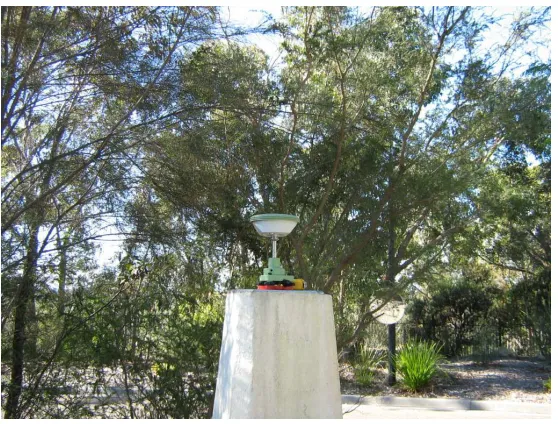
Figure 3.2: Photographic evidence of SCIMS State Survey Mark (SSM) 108024 for crosscheck on
correct occupation of marks.
The above method provided good checks for observations using tripods but when observing data on a Trigonometrical Station (TS) a.k.a. survey pillar, this method is not possible. The check used in the field was a direct measurement to the antenna base from the survey pillar base plate. The different methods of observation, static and RTK, required the changing of antennas, thus a second measurement was taken at this point providing an independent check. All independent checks and observation attributes are shown in Appendix F.
The order and time of occupation of marks in the control network are also shown in Appendix F and are included to provide the possibility of further processing using precise ephemeris data. Observation times also provided a check that the time offset setting within the instrument was correct. On the eastern coast of Australia, all time is GMT +10hrs (disregarding daylight saving time). GNSS
observations. This ensures that overlapping observation periods are sufficient to solving baselines; however this was not applied in this project due to resource constraints.
The logged data was downloaded and backed up before being made available for import into LGO.
3.4.2 RTK Static
[image:41.595.195.474.352.564.2]Due to the fact that Sydnet provides solutions for single base RTK only, the testing procedure was different from that of static observations. The occupation of network control marks was over a two-day period, the 15th and 16th of July 2008 and conducted in the same order as the static observations (See appendix F) with differing time periods.
Figure 3.3: RTK observation at TS 1582 ‘COOK’
down and would not reinitialise. The decision was made that this observation would have to suffice and a move to the next mark was made.
The next control mark, being PM 52389, proved even more frustrating with no RTK initialisation occurring despite many attempts over a 15-minute period. Once again, the mark had to be left to enable completion of the rest of the network. Fortunately, at the next control mark, TS 2868 ‘LIX’, RTK observation periods of 10 minutes were available from Chippendale and Mulgrave reference stations. Villawood, the preferred reference station, would not allow for integer ambiguities being solved.
For the remainder of observations on the 15th July 2008, there were no encountered problems with initialisation or observation periods from Chippendale and Villawood reference stations.
Figure 3.4: RTK observation at SSM 108024
SSM 24639 already had 10 minutes of data from Chippendale and over a minute from Villawood, so it was decided that 1 minute of observations would occur from Chippendale and 10 minutes from Villawood.
PM 52389 required observations at both 10 and 1-minute intervals and was done so accordingly. Unfortunately time restrictions limited the time between the occupations and all data observed was in a similar time frame, ultimately rendering the observations without an independent check. This is not good standard practice and has been noted for future reference.
The independent checks provided for static observations with respect to antenna heights were also applied to RTK observations. Although a change in antenna was all that was required in the move from static to RTK, the height of instrument was remeasured in each instance to have significant redundant measurements.
3.5
Data Processing
3.5.1 Acquisition of Sydnet data
Figure 3.5: Post processing data acquisition website
Once the chosen base station was identified, the time, in Australian Eastern Standard Time (AEST), for data acquisition was entered. Upon time selection, a choice was made between single or dual frequency requirements and the specific data rate i.e. epoch being 1 second. With confirmation that the data retrieval configurations were correct, a download box appeared and the data was sent to the designated email address.
3.5.2 Leica Geo Office (LGO)
Leica Geo Office (LGO) is a program created by Leica Geosystems for the purpose of GNSS observation data download and analysis. It provides compatibility with Leica GNSS and TPS equipment but will also handle data observed from other brands of survey equipment.
All data processing was conducted using LGO. It was important that the observation data was downloaded into a reliable processing program. LGO provided this reliability with a capability to process static data and provide housing for RTK data. It also allowed for data manipulation and verification of correct settings. A specific requirement of LGO was the ability to upload data delivered in RINEX format, which is the manner in which Sydnet provides its post process data.
The final requirement for LGO was the ability to export data in the required format (ASCII) and in a manner that supplied the relevant information i.e. point numbers, easting, northing, orthometric and ellipsoidal heights, observation times and qualities.
3.5.3 Data and Error Analysis
Errors in survey technique were minimised by ensuring that the correct network control marks had been located and that there were sufficient check measurements for receiver heights as stated in section 3.4.1. All check measurements acknowledged correct attributes for each observation allowing for the data logged at each survey mark to be downloaded and processed through LGO.
During this process the unknown ambiguities from the received carrier phase were solved and baselines calculated between occupied network control marks and CORS. All deviations from the true known value of the SCIMS marks and comparison of data are presented in Chapter 4.
3.5.4 Conformity to NSW legislation
The analysis of results in Chapter 5 will determine whether Sydnet usage complies with the current NSW legislation for accuracy and precision and whether the system is useable in certain types of survey applications.
3.6
Conclusion
Applying methods outlined by ICSM SP1 and the Surveyor General’s directions (No.9) provided a solid standard for the observation periods providing confidence in gained results.
Apart from the RTK observations at PM 52389, effectively being single occupation due to difficulties, the network control marks have been observed using techniques that are reliable and provide an independent check therefore could safely be applied in project surveys.
4.
Results
4.1
Introduction
The methods used in Chapter 3 provided observation data in real time and in raw form, which required downloading, processing and manipulation. The function of this Chapter is to present the data in a form that is presentable for easy understanding and can be assessed and analysed to determine the accuracy, precision and reliability of Sydnet by comparing the coordinate results against the known and accepted coordinates of each respective control mark.
This chapter aims to process and manipulate the raw data into a form that provides a set of
observation coordinates that can be used to compare against the known values of the control marks. Statistical calculations can then be carried out prior to the validation analysis with respect to accuracy, precision and reliability of Sydnet.
The results displayed throughout this chapter are to be presented separately in both two dimensional (horizontal) and height formats and being further divided between static and RTK observations, which have been obtained through fast static and real time methods outlined in Chapter 3. Each set of results has been processed and output through LGO to provide final coordinate sets to be used in result presentation. Through specifically chosen coordinate outputs, the data has been organised into graphical form, using Microsoft Excel, to represent horizontal and vertical results observed using both fast static and RTK observation methods.
4.2
Leica Geo Office Processing
Static observations require processing through GNSS computation software. Mentioned in Chapter 3, Leica Geo Office (LGO) was used for these computations. After the observed data had been
After a more thorough check on the equipment used and the configuration settings, it was discovered that some observations made in both static and RTK had been done so using the incorrect antenna type. Fortunately, LGO provides an option to alter properties of observations allowing the correction to occur post survey. In a project situation this is not ideal, especially when applying RTK solutions for set out type surveys. Despite the minor setback, all antenna types were corrected before processing of the static data and were also applied to RTK observations (correcting the data post process).
Due to some questionable sky clearance over some marks, it was necessary to edit the satellite windows, excluding sections of SV data that had been interrupted or scattered by overhanging trees or other objects disturbing the carrier phase waves. Interestingly, it was not only the satellite windows over the control network that needed editing but also the reference stations, specifically the
Chippendale CORS on 15th July, when it became apparent that there were two periods where no data was logged, due to circumstances unknown (shown in Figure 4.1). This had an adverse affect on some of the results.
Figure 4.1: Chippendale CORS satellite window 15/07/2008
Confident with the properties and editing of static and RTK raw test data, results were output in an ASCII format, allowing for easy readability in many software packages. For the purpose of further data manipulation, Microsoft Excel was the software package used.
4.3
Accuracy
comparison between the observed AHD heights (using Ausgeoid98 described in Chapter 3) and known AHD values of the network control marks (∆RL) will conclude accuracy results.
For the purpose of legislation and regulation compliance testing, a two dimensional vector will be calculated between the observed and known SCIMS values. This is due to fact that legislative requirements for accuracy testing are based on a misclose vector given by:
Misclose = √ (∆E) 2 + √ (∆N) 2
4.3.1 Horizontal Accuracy
Horizontal accuracy refers to the accuracy in a two dimensional manner. In most survey applications, horizontal accuracy is of great importance.
Horizontal accuracy testing required the known values of the SCIMS control network marks to be compared with the results obtained from Sydnet. An assumption has been made that all values provided by SCIMS are true and correspond to their respective class and order and have been accepted. Comparisons have been made between:
i) average observed coordinates obtained using static and RTK methods ii) observed coordinates obtained from individual CORS using static and RTK iii) a comparison between static and RTK observation results
Average Static Observations
The results show that the observation set as a whole averaged a difference in easting of -11.1mm and a northing difference of 2.7mm with single standard deviations of 15.4mm and 17.8mm respectively. Figure 4.2 is a graphical representation of the results shown in Appendix H. One standard deviation (σ) has been shown for each individual data set i.e. σE for PM 52389 differs from σE for SSM 108024 as shown in Appendix H.
2D Average Observations v SCIMS Coordinates
-0.060 -0.050 -0.040 -0.030 -0.020 -0.010 0.000 0.010 0.020 0.030 0.040 P M 5 2 3 8 9 S S M 1 0 8 0 2 4 S S M 2 4 6 3 9 T S 1 1 0 0 T S 1 5 8 2 T S 2 8 6 8 T S 2 8 8 8 T S 2 9 6 2
Network Control Marks
D if fe re n c e ( m )
∆
E
∆
N
Figure 4.2: Average two-dimensional static observed coordinates and respective σ
Individual Static Observations
To determine the accuracy of results observed from individual reference stations, a test was applied where each control mark was fixed by the average baseline solution from each individual CORS. This test was applied to determine whether any systematic errors were present when adopting specific reference stations.
Individual Baseline Calculations for PM 52389 v SCIMS Coordinates
-0.030 -0.020 -0.010 0.000 0.010 0.020 0.030 0.040
Chippendale Villaw ood Cow an Mulgrave
Reference Base Station
D
iffe
re
n
c
e
(m
)
∆E
∆N
Figure 4.3: Individual static baseline calculations to PM 52389 and respective σ
Average RTK Observations
The test for average RTK observations was virtually a repeat of the above test for static observations with the exception of number of baselines. Due to the fact that RTK is provided by a single base only, observations were limited to the solving of two baselines as shown in chapter 3, section 3.4.2.
2D Average Observations v SCIMS Coordinates -0.060 -0.050 -0.040 -0.030 -0.020 -0.010 0.000 0.010 0.020 0.030 0.040 P M 5 2 3 8 9 S S M 1 0 8 0 2 4 S S M 2 4 6 3 9 T S 1 1 0 0 T S 1 5 8 2 T S 2 8 6 8 T S 2 8 8 8 T S 2 9 6 2
Network Control Marks
D if fe re n c e ( m )
∆
E
∆
N
Figure 4.4: Average two-dimensional RTK observed coordinates and respective σ
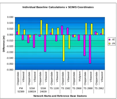
Individual RTK Observations
The individual baselines for RTK observations differ slightly to the static observations in that there were fewer baselines calculated however, the test intended to provide the same desired outcome as the individual static observations.
Individual Baseline Calculations v SCIMS Coordinates -0.060 -0.050 -0.040 -0.030 -0.020 -0.010 0.000 0.010 0.020 0.030 C h ip p e n d a le V il la w o o d C h ip p e n d a le V il la w o o d C h ip p e n d a le V il la w o o d C h ip p e n d a le V il la w o o d C h ip p e n d a le V il la w o o d C h ip p e n d a le M u lg ra v e C h ip p e n d a le V il la w o o d C h ip p e n d a le V il la w o o d PM 52389 SSM 108024 SSM 24639
TS 1100 TS 1582 TS 2868 TS 2888 TS 2962
Network Marks and Reference Base Stations
[image:54.595.131.537.64.407.2]D if fe re n c e ( m ) ∆E ∆N
Figure 4.5: Average RTK single baseline solutions over two separate observations
Static Observations v RTK Observations
The final test for two-dimensional accuracy was a comparison of average static observation positioning and average RTK observation positioning. This test has been devised to provide a direct comparison between fast static and RTK static observations, which may impact on the chosen method of survey in project application.
Static and RTK Observations v SCIMS Coordinates -0.060 -0.050 -0.040 -0.030 -0.020 -0.010 0.000 0.010 0.020 0.030 0.040 S ta ti c R T K S ta ti c R T K S ta ti c R T K S ta ti c R T K S ta ti c R T K S ta ti c R T K S ta ti c R T K S ta ti c R T K PM 52389 SSM 108024 SSM 24639
TS 1100 TS 1582 TS 2868 TS 2888 TS 2962
Network Marks and Method of Observation
[image:55.595.131.537.65.398.2]D if fe re n c e ( m ) ∆E ∆N
Figure 4.6: Average static observations & average RTK observations compared to SCIMS MGA
values of network control marks
4.3.2 Vertical Accuracy
Vertical accuracy in GNSS surveys can refer to many datum’s. The generally accepted height
comparisons for GNSS surveys relate to the height of the antenna above the reference ellipsoid, which in this case is the GRS80. Ellipsoid height however does not provide a realistic height on the earth’s surface. Orthometric heights, are a measure of height above (or below) the geoid (Ausgeoid98 for this project) and are given by the equation:
Orthometric Height = Ellipsoidal Height – N
For the purposes of this paper, orthometric heights were calculated, using the N values determined in Ausgeoid98 <http://www.ga.gov.au>, providing a RL at each mark for comparison with the known AHD value at each mark. Within NSW many surveys requiring a height component are required to be on AHD and for that reason all observations at network control marks will be compared on that datum. The Ausgeoid98 model is installed within LGO and N values are simply computed based on the coordinate position of marks.
As an independent check that the Ausgeoid98 model was correct within LGO, the N values were obtained from the geosciences website (shown in Appendix E) for each network control mark and manually applied to the observed ellipsoidal height. In all instances the LGO calculated orthometric height was equivalent to the manually calculated heights.
As with horizontal accuracy, vertical accuracy results must show that the data received can be relied upon for surveys requiring a height component. For this purpose, height data, also referred to as a Reduced Level (RL) was compared to known SCIMS values of network control marks in the same fashion as the horizontal results as follows:
i) average AHD height observations obtained using static and RTK methods ii) AHD heights obtained from individual CORS using static and RTK iii) a comparison between static and RTK observation results
Average Static Heights
As with the averaged two-dimensional coordinates, the heights from all static baselines were averaged to determine the overall accuracy with respect to height at each control mark. This test was to
The heights of each reference station used in processing have been levelled according to local AHD values by static observations adopting existing local high accuracy marks over lengthy periods of time (see Chapter 2, section 2.4), so the averaging of the heights effectively provides a network solution for the individual height values obtained by observation, keeping in mind that results have not been weighted.
The average heights when compared to the SCIMS value at each network control mark produced results as follows:
Average Observed AHD Values v SCIMS AHD Values
-0.250 -0.200 -0.150 -0.100 -0.050 0.000 0.050 P M 5 2 3 8 9 S S M 1 0 8 0 2 4 S S M 2 4 6 3 9 T S 1 1 0 0 T S 1 5 8 2 T S 2 8 6 8 T S 2 8 8 8 T S 2 9 6 2
Network Control Marks
[image:57.595.139.530.284.626.2]D if fe re n c e ( m ) ∆RL
Figure 4.7: Average static height observations and respective σ
Individual Static Heights
Observed heights from individual reference stations are shown in Figure 4.8. This test is an important one and outlines the differences that can occur in height determination when adopting a specific reference station. Although heights do show some trend between the separate CORS, it is not specifically systematic with height differences appearing somewhat random in areas.
Individual Baseline Static Calculations v SCIMS Coordinates
-0.200 -0.150 -0.100 -0.050 0.000 0.050 C h ip p e n d a le V il la w o o d C o w a n M u lg ra v e C h ip p e n d a le V il la w o o d C o w a n M u lg ra v e C h ip p e n d a le V il la w o o d C o w a n M u lg ra v e C h ip p e n d a le V il la w o o d C o w a n M u lg ra v e C h ip p e n d a le V il la w o o d C o w a n M u lg ra v e C h ip p e n d a le V il la w o o d C o w a n M u lg ra v e C h ip p e n d a le V il la w o o d C o w a n M u lg ra v e C h ip p e n d a le V il la w o o d C o w a n M u lg ra v e
PM 52389 SSM 108024
SSM 24639
TS 1100 TS 1582 TS 2868 TS 2888 TS 2962
Network Marks and Reference Base Stations
D if fe re n c e ( m
[image:58.595.128.538.222.532.2]) ∆RL
Figure 4.8: Individual baseline height observations
These results prove that the height determination from each CORS differ greatly when processed in their raw form. As stated in Phipps’ paper (2008), the errors associated with these findings are yet to be uncovered i.e. why do AHD values differ so greatly in different areas of Sydney?
Average RTK Heights
Results show similar quality to that of static results in that all residuals are negative and are ranged between -22mm and -114mm and having a mean of -72.3mm. Figure 4.9 below provides a graph of the above results with a single standard deviation.
Observed AHD Values v SCIMS AHD Values
-0.250 -0.200 -0.150 -0.100 -0.050 0.000 0.050 0.100 0.150 P M 5 2 3 8 9 S S M 1 0 8 0 2 4 S S M 2 4 6 3 9 T S 1 1 0 0 T S 1 5 8 2 T S 2 8 6 8 T S 2 8 8 8 T S 2 9 6 2
Network Control Marks
[image:59.595.139.526.197.537.2]D if fe re n c e ( m ) ∆RL
Figure 4.9: Average RTK observed heights and respective σ
Individual RTK Heights
Individual Base line Calculations v SCIM S Coordinates -0.200 -0.150 -0.100 -0.050 0.000 0.050 0.100 C h ip p e n d a le V il la w o o d C h ip p e n d a le V il la w o o d C h ip p e n d a le V il la w o o d C h ip p e n d a le V il la w o o d C h ip p e n d a le V il la w o o d C h ip p e n d a le M u lg ra v e C h ip p e n d a le V il la w o o d C h ip p e n d a le V il la w o o d PM 52389 SSM 108024 SSM 24639
TS 1100 TS 1582 TS 2868 TS 2888 TS 2962
Network Marks and Reference Base Stations
[image:60.595.132.538.70.486.2]D if fe re n c e ( m ) ∆RL
Figure 4.10: Individual RTK height observations to all network control marks
Results from this test seem poor and provide little confidence in RTK height ability with large differences between both individual baselines when compared to SCIMS and individual baselines when compared to each other. Unlike all other results to now, there are two positive residuals in this data set.
Static Height Observations v RTK Height Observations
static and RTK static observations, which may impact on the chosen method of survey in project application.
Figure 4.11 provides the results of the observations at each control mark using each method, side by side to allow easy comparison. These results typically reveal what accuracies could be expected when using either method.
As could be expected from the above previous tests, overall heighting from Sydnet appears
Static and RTK Observations v SCIMS Coordinates -0.160 -0.140 -0.120 -0.100 -0.080 -0.060 -0.040 -0.020 0.000 S ta ti c R T K S ta ti c R T K S ta ti c R T K S ta ti c R T K S ta ti c R T K S ta ti c R T K S ta ti c R T K S ta ti c R T K PM 52389 SSM 108024 SSM 24639
TS 1100 TS 1582 TS 2868 TS 2888 TS 2962
Network Marks and Method of Observation
[image:62.595.131.536.69.457.2]D if fe re n c e ( m ) ∆RL
Figure 4.11:Average static observations & average RTK observations compared to SCIMS AHD71
values of network control marks
4.4
Precision
Precision is a measure of observation repeatability. An example of good precision is when repeated observations are taken at different periods and provide similar results. Generally the standard deviation of an observation set is a reliable measure of precision with high standard deviation values equating to low precision observations and vice versa.
i) Precision of two dimensional static observations ii) Precision of two dimensional RTK observations iii) Precision of static height observations
iv) Precision of RTK height observations
Precision of Static Observations
The test for precision of static observations has been viewed in two manners; one being the standard deviation calculation for the average observation at each control mark and the other being a
comparison of observed coordinates from day to day.
[image:63.595.131.536.406.705.2]Results shown in Figure 4.12 reveal the 95% confidence interval as per ICSM SP1, for two-dimensional static observations. The 95% confidence interval for GNSS observations is 2.45 x Standard Deviation of the observation set, to conform to ICSM SP1.
Figure 4.12: 95% confidence interval of average static observations
95% Confidence Interval Static Obse rvations
0.0000 0.0050 0.0100 0.0150 0.0200 0.0250 0.0300 0.0350 0.0400 0.0450 0.0500 P M 5 2 3 8 9 S S M 1 0 8 0 2 4 S S M 2 4 6 3 9 T S 1 1 0 0 T S 1 5 8 2 T S 2 8 6 8 T S 2 8 8 8 T S 2 9 6 2
Network Control Marks
(m
) 95% CI ∆E
The above results show that the repeatability of observations appears good except for SSM 108024, which has higher than expected standard deviations. Possible reasons for less precise results are outlined in Chapter 5.
Results on a day to day basis reveal the repeatability of the system and are shown in the following graph (Figure 4.13), which also shows the variance from the known SCIMS values of network control marks.
Daily 2D Observations v SCIMS coordinates
-0.060 -0.050 -0.040 -0.030 -0.020 -0.010 0.000 0.010 0.020 0.030 0.040 15- Jul-08 16- Jul-08 15- Jul-08 16- Jul-08 15- Jul-08 16- Jul-08 15- Jul-08 16- Jul-08 15- Jul-08 16- Jul-08 15- Jul-08 16- Jul-08 14- Jul-08 15- Jul-08 16- Jul-08 15- Jul-08 16- Jul-08 PM 52389 SSM 108024 SSM 24639
TS 1100 TS 1582 TS 2868 TS 2888 TS 2962
Network Control Mark and Date of Observation
[image:64.595.138.528.279.634.2]D if fe re n c e ( m ) ∆E ∆N
Precision of RTK Observations
The tests for precision of RTK results are much the same as that of static observations firstly viewing the standard deviations of averaged positions and then comparing daily results. Due to the fact that RTK solution was not possible at PM 52389 on the 15th July, it has been omitted from the results.
95% Confidence Interval RTK Observations
0.0000 0.0050 0.0100 0.0150 0.0200 0.0250 0.0300 0.0350 0.0400 0.0450 0.0500 S S M 1 0 8 0 2 4 S S M 2 4 6 3 9 T S 1 1 0 0 T S 1 5 8 2 T S 2 8 6 8 T S 2 8 8 8 T S 2 9 6 2
Network Control Marks
(m
) 95% CI ∆E
[image:65.595.129.538.251.544.2]95% CI ∆N
Figure 4.14: 95%Confidence Interval of average RTK observations
(Excluding PM 52389)
Daily 2D RTK Observations v SCIMS coordinates -0.060 -0.050 -0.040 -0.030 -0.020 -0.010 0.000 0.010 0.020 0.030 0.040 15- Jul-08 16- Jul-08 15- Jul-08 16- Jul-08 15- Jul-08 16- Jul-08 15- Jul-08 16- Jul-08 15- Jul-08 16- Jul-08 15- Jul-08 16- Jul-08 15- Jul-08 16- Jul-08 SSM 108024 SSM 24639
TS 1100 TS 1582 TS 2868 TS 2888 TS 2962
Network Control Mark and Date of Observation
[image:66.595.139.526.71.406.2]D if fe re n c e ( m ) ∆E ∆N
Figure 4.15: Day to day comparison of RTK observations and standard deviation of data sets
Precision of Static Heights
95% Confidence Interval Static Observations
0.0000 0.0200 0.0400 0.0600 0.0800 0.1000 0.1200 0.1400 0.1600 0.1800