16th Australasian Fluid Mechanics Conference Crown Plaza, Gold Coast, Australia
2-7 December 2007
Radial-basis-function Calculations of Buoyancy-driven Flow in Concentric and Eccentric
Annuli
K. Le-Cao, N. Mai-Duy and T. Tran-Cong
Computational Engineering and Science Research Centre University of Southern Queensland, Queensland, 4350 AUSTRALIA
Abstract
This paper is concerned with the application of integrated radial-basis-function networks (IRBFNs) for the simulation of natural convection in concentric and eccentric annuli. Important features of the present technique include: (i) Taking a stream function - temperature formulation as the governing equations; (ii) Employing a Cartesian grid to discretize the problem do-main; (iii) Using one-dimensional RBF approximations to rep-resent the approximate solution; and (iv) Constructing the ap-proximations through integration. These features result in an efficient numerical scheme as (i) the number of the governing differential equations is reduced from 4 to 2, (ii) the preprocess-ing is simple, (iii) the associated matrices have condition num-bers in 2-norm that are much lower than those yielded through conventional RBF techniques, and (iv) the reduction of conver-gence rate caused by differentiation is avoided. A wide range of the Rayleigh number is considered. Results obtained are com-pared well with available numerical data in literature.
Keywords: Natural convection; Cartesian grid method; Irregu-lar domain; Integrated radial basis function networks
Introduction
Natural convection is an important phenomenon in many ap-plications in engineering and science such as meteorology, nu-clear reactors and solar energy systems. The problem has thus been extensively studied by both experimental and theoretical approaches. The motion of a fluid is caused by the combination of density variations and gravity. Natural convection is gov-erned by the coupling of momentum equation (velocity field) and energy equation (temperature field). Numerical solutions can be achieved by means of discretisation, followed by solu-tions of the resultant algebraic equasolu-tions. Results have been reported using different discretisation techniques such as finite-difference methods (FDMs) (e.g. [1,10]), finite-element meth-ods (FEMs) (e.g. [17,22]), finite-volume methmeth-ods (FVMs) (e.g. [4,6]), boundary-element methods (BEMs) (e.g. [5,9,20]) and spectral methods (e.g. [11,24]).
RBFNs have been proved to be a universal approximator. Over the last fifteen years, the networks have been developed to solve different types of differential problems encountered in applied mathematics, science and engineering (e.g. [3,7,8,13,23,27]). RBFN methods are truly meshless, extremely easy to imple-ment and capable of achieving a high level of accuracy using relatively small numbers of nodes. However, the RBF sys-tem matrix is fully populated and its condition number grows rapidly as the number of nodes is increased. One way to over-come these problems is to approximate the solution locally. Re-cently, one-dimensional (1D) IRBFN approximation schemes have been proposed in [16]. The “local” 1D-IRBFN approxi-mations at a grid node involve only nodal points that lie on the grid lines intersected at that point rather than the whole set of nodes. Moreover, the construction of the RBF approximations is based on integration, which avoids the reduction of conver-gence rate caused by differentiation. Numerical results have indicated that this approach allows larger numbers of nodes to
be employed and is able to maintain a fast rate of convergence with grid refinement.
In this paper, we present the 1D-IRBFN technique for the sim-ulation of buoyancy-driven flow governed by nonlinear par-tial differenpar-tial equations (PDEs) and defined in concentric and eccentric annuli. For conventional FDMs and pseudospectral techniques, coordinate transformations are required to convert non-rectangular domains into rectangular ones [18,26]. The re-lationships between the physical and computational coordinates are given by a set of algebraic equations or a set of PDEs, de-pending on the level of complexity of the geometry. Such trans-formation processes are, in general, complicated. By contrast, the present method is able to retain the PDEs in their Cartesian forms, and thus work in a similar fashion for different shapes of annuli. In addition, the formulation of stream function and temperature is employed, which reduces the number of depen-dent variables from four (two velocity components, pressure and temperature) to two (stream function and temperature). An outline of the paper is as follows. First, a brief review of the governing equations is given. Then, the present 1D-IRBFN technique is described, followed by numerical results for nat-ural convection in circular-circular and square-circular annuli. Finally, some remarks conclude the paper.
Governing Equations
Using the Boussinesq approximation, the 2D dimensionless forms of the PDEs governing buoyancy-driven flows can be written as (e.g. [19])
∂u
∂x+
∂v
∂y=0, (1)
∂u
∂t+u
∂u
∂x+v
∂u
∂y =−
∂p
∂x+
r
Pr Ra
∂2u ∂x2+
∂2u ∂y2
, (2) ∂v
∂t+u
∂v
∂x+v
∂v
∂y=−
∂p
∂y+
r
Pr Ra
∂2v ∂x2+
∂2v ∂y2
+T, (3) ∂T
∂t +u
∂T
∂x+v
∂T
∂y =
1
√ RaPr
∂2T ∂x2 +
∂2T ∂y2
, (4) where u and v are the velocity components, p the dynamic pres-sure, T the temperature, and Pr and Ra the Prandtl and Rayleigh numbers defined as Pr=ν/αand Ra=βg∆T L3/αν, respec-tively in whichνis the kinematic viscosity,αthe thermal dif-fusivity,βthe thermal expansion coefficient, g the gravity, and
L and∆T the characteristic length and temperature difference,
respectively. In this dimensionless scheme, the velocity scale is taken as U=pgLβ∆T for the purpose of balancing the
buoy-ancy and inertial forces.
By writing the velocity components in terms of a stream func-tionψdefined as
u=∂ψ
∂y, v=−
∂ψ ∂x,
momen-tum equations reduce to ∂
∂t
∂2ψ ∂x2 +
∂2ψ ∂y2
+∂ψ ∂y
∂3ψ ∂x3 +
∂3ψ ∂x∂y2
−∂ψ∂ x
∂3ψ ∂x2∂y+
∂3ψ ∂y3
= r
Pr Ra
∂4ψ ∂x4 +2
∂4ψ ∂x2∂y2+
∂4ψ ∂y4
−∂∂T
x. (5)
It can be seen that one can replace the system of four equations (1)-(4) by a set of two equations (4) and (5). The latter will be employed in the present work.
The Present 1D-IRBFN Technique
One-dimensional IRBFNs
It is known that RBFNs have the property of universal approx-imation. The RBFN allows the conversion of a function to be approximated from a low-dimensional space (e.g., 1D here) to a high-dimensional space in which the function is expressed as a linear combination of RBFs
f(x) =
m
∑
i=1
wigi(x), (6)
where m is the number of RBFs,{gi(x)}mi=1the set of RBFs, and
{wi}mi=1the set of weights to be found. The present technique implements the multiquadric (MQ) function whose form is
gi(x) =
q
(x−ci)2+a2i, (7)
where ci and ai are the centre and the width of the ith basis
function.
In the traditional/direct approach, a function f is approximated by an RBFN, followed by successive differentiations to obtain approximate expressions for its derivatives. There is a reduction in convergence rate for derivative functions and this reduction is an increasing function of derivative order [12].
Mai-Duy and Tran-Cong [14,15] have proposed the use of inte-gration to construct the RBF approximations. A derivative of f is decomposed into RBFs, and lower-order derivatives and the function itself are then obtained through integration
dpf(x)
dxp = m
∑
i=0
wigi(x) = m
∑
i=0
wiI
(p)
i (x), (8)
dp−1f(x)
dxp−1 =
m
∑
k=0
wiIi(p−1)(x) +c1, (9)
dp−2f(x)
dxp−2 =
m
∑
k=0
wiIi(p−2)(x) +c1x+c2, (10)
··· ··· ··· ··· ···
d f(x)
dx =
m
∑
k=0
wiIi(1)(x) +c1
xp−2
(p−2)!+c2
xp−3
(p−3)!+···+
cp−2x+cp−1, (11)
f(x) =
m
∑
k=0
wiIi(0)(x) +c1
xp−1
(p−1)!+c2
xp−2
(p−2)!+···+
cp−1x+cp, (12)
where Ii(p−1)(x) = R
Ii(p)(x)dx, Ii(p−2)(x) = R
Ii(p−1)(x)dx,···,Ii(0)(x) = R
Ii(1)(x)dx, and c1,c2,···,cp
are the constants of integration. Numerical results have shown that the integral approach significantly improves the quality of the approximation of derivative functions over conventional
differential approaches. The IRBF approximation scheme is said to be of pth-order, denoted by IRBFN-p, if the pth-order derivative is taken as the staring point.
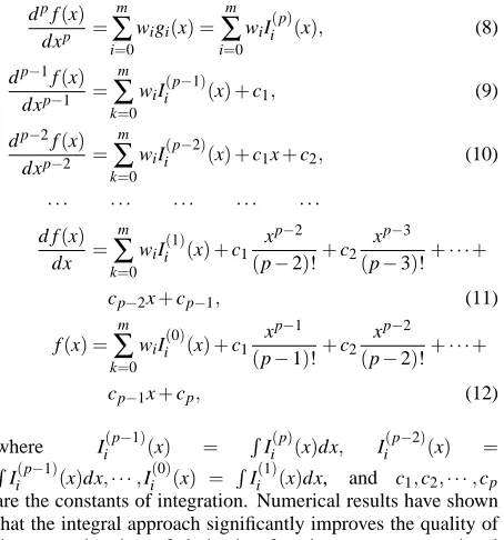
[image:2.595.59.286.524.767.2]Simulation of Buoyancy-driven Flow
Figure 1: A circular-circular annulus: Computational domain and discretisations: 11×11 (left) and 61×61 (right).
Consider the process of natural convection between two cylin-ders, one heated and the other cooled (e.g. Figure 1). The problem domain is embedded in a Cartesian grid with a grid spacing h. Grid points outside the domain (external points) to-gether with internal points that fall very close–within a distance of h/8–to the boundary are removed. The remaining grid points are taken to be the interior nodes. The boundary nodes consist of the grid points lying on the boundaries, and points generated by the intersection of the grid lines with the boundaries. Along each grid line, 1D-IRBFNs are employed to approximate the solutions and their relevant derivatives. In what follows, the proposed method is described in detail for the energy equation (4) and the momentum equation (5). Special attention is given to the implementation of boundary conditions.
IRBFN Discretisation of The Energy Equation
The energy equation involves the following linear second-order differential operator
L
2= ∂ 2 ∂x2+∂2
∂y2. (13)
As presented earlier, an IRBFN-p scheme permits the approxi-mation of a function and its derivatives of orders up to p. To use integrated basis functions only, one needs to employ IRBFNs of at least second order. A line in the grid contains two sets of points (Figure 2). The first set consists of the interior points that are also the grid nodes (regular nodes). The values of the tem-perature at the interior points are unknown. The second set is formed from the boundary nodes that do not generally coincide with the grid nodes (irregular nodes). At the boundary nodes, the values of the temperature are given.
For classical FDMs, the irregular nodes require changes of∆x
and∆y in the finite-difference formulas, and such changes
de-teriorate the order of truncation error [22]. Unlike FD and also spectral approximation schemes, IRBFNs have the capability to handle unstructured points with high accuracy. As a result, the present technique does not require any special treatments for ir-regular boundary points. The boundary conditions are imposed through the process of converting the network-weight space into the physical space (conversion process).
x1 x2 xq
[image:3.595.55.266.154.354.2]xb1 xb2
Figure 2: Points on a grid line consist of interior points xi(◦)
and boundary points xbi(2).
constructed as follows
b
T
b
Tb
=
C
bwb, (14)where b
T= T1,T2,···,Tq
T
, b
Tb= (Tb1,Tb2)T,
b
w= (w1,w2,···,wm,c1,c2)T,
b
C
= I1(0)(x1) ··· I (0)
m (x1) x1 1
I1(0)(x2) ··· Im(0)(x2) x2 1
··· ··· ··· ··· ···
I1(0)(xq) ··· Im(0)(xq) xq 1
I1(0)(xb1) ··· I
(0)
m (xb1) xb1 1
I1(0)(xb2) ··· I
(0)
m (xb2) xb2 1
,
and m=q+2.
The obtained system (14) for the unknown vector of network weights can be solved using the singular value decomposition technique
b
w=
C
b−1b T b Tb . (15)
Taking (15) into account, the values of the first and second derivatives of T at the interior points are computed by
∂T1
∂x
∂T2
∂x
.. .
∂Tq
∂x =b
I
(1)[2]
C
b− 1 Tbb Tb , (16) and
∂2T 1
∂x2
∂2T 2
∂x2
.. .
∂2T q
∂x2
=b
I
(2)[2]
C
b− 1 Tbb Tb , (17) where b
I
(1) [2] = I1(1)(x1) ··· Im(1)(x1) 1 0
I1(1)(x2) ··· I (1)
m (x2) 1 0
··· ··· ··· ··· ···
I1(1)(xq) ··· Im(1)(xq) 1 0
, and b
I
(2) [2] = I1(2)(x1) ··· Im(2)(x1) 0 0
I1(2)(x2) ··· Im(2)(x2) 0 0
··· ··· ··· ··· ···
I1(2)(xq) ··· Im(2)(xq) 0 0
.
Expressions (16) and (17) can be rewritten in compact forms c
∂T
∂x =
D
b1xTb+bk1x, (18)and
d ∂2T
∂x2 =
D
b2xTb+bk2x, (19) wherebk1xandbk2xare the vectors of known quantities related to boundary conditions.It can be seen from (18) and (19) that the IRBFN approxima-tions of∂T/∂x and∂2T/∂x2 at the interior points include in-formation about the inner and outer boundaries (locations and boundary values). Thus it remains only to force these approxi-mations to satisfy the governing equation.
The incorporation of the boundary points into the set of centres has several advantages:
• It allows the two sets of centres and collocation points to be the same, i.e.{ci}mi=1≡
n
{xi}qi=1∪ {xbi}2i=1 o
. Numer-ical investigations [16,23] have indicated that, when these two sets coincide, the RBF approximation scheme tends to result in the most accurate approximate solution.
• It allows the use of IRBFNs with a fixed order (IRBFN-2), regardless of the shape of the domain.
In the same manner, one can obtain the IRBF expressions for ∂T/∂y and∂2T/∂y2at the interior points along a vertical line. As with FDMs, FVMs, BEMs and FEMs, the IRBF approxi-mations will be gathered together to form the global matrices for the discretisation of the PDE. By collocating the govern-ing equation at the interior points, a square system of algebraic equations is obtained, which is solved for the approximate tem-perature at the interior points.
IRBFN Discretisation of The Momentum Equation
The momentum equation involves the following linear fourth-order differential operator
L
4= ∂ 4 ∂x4+2∂4 ∂x2∂y2+
∂4
∂y4. (20) At each boundary node, the solution is required to satisfy two prescribed values, ψand ∂ψ/∂n. It is straightforward to
ob-tain the values of∂ψ/∂x and∂ψ/∂y at the boundary nodes from
the prescribed conditions. The double boundary conditions are implemented through the conversion process of the network-weight space into the physical space.
Along each grid line, the set of centres also consists of the in-terior points and the boundary points. The addition of extra equations to the conversion system for the purpose of represent-ing derivative boundary conditions is offset by the generation of additional unknowns of the integral collocation approach. Con-sider a horizontal grid line (Figure 2). The present work em-ploys 1D-IRBFN-4s to approximate the variableψ. The con-version system is given by
b ψ b ψb
d∂ψb
∂x
=
C
bwb, (21)where
b
ψ= ψ1,ψ2,···,ψqT,
b
ψb= (ψb1,ψb2)T,
∂bψb
∂x =
∂ψ
b1
∂x ,
∂ψb2
∂x
T
,
b
b
C
= I1(0)(x1) ··· Im(0)(x1) x31/6 x21/2 x1 1
I1(0)(x2) ··· Im(0)(x2) x32/6 x22/2 x2 1
··· ··· ··· ··· ···
I1(0)(xq) ··· Im(0)(xq) x3q/6 x2q/2 xq 1
I1(0)(xb1) ··· I
(0)
m (xb1) x3b1/6 x2b1/2 xb1 1
I1(0)(xb2) ··· I
(0)
m (xb2) x3b2/6 x
2
b2/2 xb2 1
I1(1)(xb1) ··· I
(1)
m (xb1) x2b1/2 xb1 1 0
I1(1)(xb2) ··· I
(1)
m (xb2) x2b2/2 xb2 1 0
,
and m=q+2. The values of the lth-order derivative (l=
{1,2,3,4}) ofψat the interior points on the line are evaluated as
d ∂4ψ ∂x4 =b
I
(4) [4]
C
b−1 b ψ b ψb
d∂ψb
∂x
, (22)
d ∂3ψ ∂x3 =b
I
(3) [4]
C
b−1 b ψ b ψb
d∂ψb
∂x
, (23)
d ∂2ψ ∂x2 =b
I
(2) [4]
C
b−1 b ψ b ψb
d∂ψb
∂x
, (24)
and
d ∂1ψ ∂x1 =b
I
(1) [4]
C
b−1 b ψ b ψb
d∂ψb
∂x
, (25)
where b
I
(4) [4] = I1(4)(x1)···Im(4)(x1) 0 0 0 0
I1(4)(x2)···I (4)
m (x2) 0 0 0 0
··· ··· ··· ··· ···
I1(4)(xq)···Im(4)(xq) 0 0 0 0
, b
I
(3) [4] = I1(3)(x1)···Im(3)(x1) 1 0 0 0
I1(3)(x2)···Im(3)(x2) 1 0 0 0
··· ··· ··· ··· ···
I1(3)(xq)···Im(3)(xq) 1 0 0 0
, b
I
(2) [4] = I1(2)(x1)···Im(2)(x1) x1 1 0 0
I1(2)(x2)···Im(2)(x2) x2 1 0 0
··· ··· ··· ··· ···
I1(2)(xq)···Im(2)(xq) xq 1 0 0
, and b
I
(1) [4] = I1(1)(x1)···I (1)
m (x1) x21/2 x1 1 0
I1(1)(x2)···Im(1)(x2) x22/2 x2 1 0
··· ··· ··· ··· ···
I1(1)(xq)···Im(1)(xq) x2q/2 xq 1 0
.
Expressions (22)-(25) can reduce to d
∂lψ
∂xl =
D
blxψb+bklx, (26)wherebklxare the vectors of known quantities related to
bound-ary conditions. Since the discretisation used has a structured form, the process of joining “local” 1D-IRBF approximations together (assemblage process) is quite straightforward. For a special case of rectangular domain, the IRBF approximations
over a 2D domain can simply be constructed using the tensor direct product.
The fourth- and also third-order mixed derivatives are computed using the following relations
∂4ψ ∂2x∂2y=
1 2
∂2 ∂x2
∂2ψ ∂y2
+ ∂
2 ∂y2
∂2ψ ∂x2
, (27) ∂3ψ
∂2x∂y= ∂2 ∂x2
∂ψ
∂y
, (28)
∂3ψ ∂x∂y2=
∂2 ∂y2
∂ψ
∂x
. (29)
Expressions (27)-(29) reduce the computation of mixed deriva-tives to that of lower-order pure derivaderiva-tives for which IRBFNs involve integration with respect to x or y only. The ad-ditional work here is the computation of ∂2(F)/∂x2 and ∂2(F)/∂y2 where F is a derivative function of ψ (i.e. ∂2ψ/∂y2,∂2ψ/∂x2,∂ψ/∂y and∂ψ/∂x). It can be seen that the discretisation of (5) requires the values of the mixed derivatives at the interior points. IRBFN-2s can be employed here to con-struct the approximations for∂2(F)/∂x2and∂2(F)/∂y2. Both sets of centres and collocation points of these second-order net-works consist of the interior nodes only. The IRBF expressions for derivatives are now written in terms of the values ofψat the interior points, and they already satisfy the boundary con-ditions. These nodal variable values are determined by forcing the approximate solution to satisfy the momentum equation at the interior points. Like the energy equation, the resultant sys-tem of algebraic equations here is of size nip×nip, where nipis
the number of interior points of the domain. Solution Procedure
The energy and momentum equations must be solved simulta-neously to find the values of the temperature and stream func-tion at discrete points within the domain. Because of the pres-ence of convective terms in the governing equations, the ob-tained algebraic equations for the discrete solution are nonlin-ear. In this paper, a time dependent decoupled approach is em-ployed to handle this nonlinearity. The advantage of this ap-proach is that it allows the breakdown of the problem into the solution of the energy equation and the solution of the momen-tum equation (two smaller subproblems at each iteration). The nonlinear equation set is solved in a marching manner.
1. Guess initial values of T,ψ and their first-order spatial derivatives at time t=0.
2. Discretize the governing equations in time using a first-order accurate finite-difference scheme, where the diffu-sive and convective terms are treated implicitly and ex-plicitly, respectively.
3. Discretize the governing equations in space using 1D-IRBF schemes:
Solve the energy equation (4) for T , and Solve the momentum equation (5) forψ.
The two equations are solved separately in order to keep matrix sizes to a minimum.
4. Check to see whether the solution has reached a steady state
CM= r
∑nip
i=1
ψ(k)
i −ψ
(k−1)
i
2
r ∑nip
i=1
ψ(k)
i
where k is the time level andεis the tolerance.
5. If it is not satisfied, advance time step and repeat from step 2. Otherwise, stop the computation and output the results.
Numerical Results
The present method is applied to the simulation of buoyancy-driven flow in concentric and eccentric annuli. A wide range of the Rayleigh number is considered. The computed solution at the lower and nearest value of Ra is taken to be the initial solution. The MQ-RBF width is simply chosen to be the grid size h.
Natural Convection in A Circular Annulus
Consider the natural convection between two concentric cylin-ders which are separated by a distance L, the inner cylinder heated and the outer cylinder cooled (Figure 1). A comprehen-sive review of this problem can be found in [10]. Most cases have been reported with Pr=0.7 and L/Di=0.8, in which
Diis the diameter of the inner cylinder. These conditions are
also employed in the present work. Kuehn and Goldstein [10] have also reported numerical results by FDM for Ra=102 to
Ra=7×10⁴. Using the differential quadrature method (DQM), Shu [24] has provided very accurate solutions for values of the Rayleigh number in the range of 102to 5×10⁴.
One typical quantity associated with this type of flow is the av-erage equivalent conductivity denoted by ¯keq. This quantity is
defined as ([10,24]) ¯keq= −
ln(Do/Di)
2π I
∂T
∂nds (31)
in which Dois the diameter of the outer cylinder.
0 1000 2000 3000 4000 5000 6000 10−14
10−12
10−10
10−8 10−6 10−4 10−2 100
Number of iterations
C
M
Figure 3: Iterative convergence. Time steps used are 0.5 for
Ra={102,103,3×103}, 0.1 for Ra={6×103,104}, and 0.05 for Ra={5×104,7×104}. The values of CM become less than 10−12when the numbers of iterations reach 58, 154, 224, 1276, 1541, 5711 and 5867 for Ra={102,103,3×103,6×
103,104,5×104,7×104}, respectively.
[image:5.595.341.509.120.287.2]The stream function and its normal derivative are set to zero along the inner and outer cylinders. The temperature is held at T=1 at the inner cylinder and T=0 at the outer cylin-der. We employ a number of uniform Cartesian grids, namely 11×11,21×21,···,61×61, to study the behaviour of grid con-vergence of the present method. The concon-vergence of the itera-tive procedure with respect to time step is shown in Figure 3.
Figure 4: An eccentric square-circular annulus: Computational domain and discretisation
The condition numbers of matrices associated with harmonic (13) and biharmonic (20) operators in the governing equations (4) and (5) are reported in Table 1.
Grid cond(
L
2T ) cond(L
4ψ)11×11 1.3×101 7.4×101 21×21 1.2×10² 5.0×10³ 31×31 3.3×10² 3.3×10⁴ 41×41 5.1×10² 7.9×10⁴ 51×51 7.5×10² 1.6×10⁵ 61×61 1.0×10³ 3.2×10⁵
Table 1: Circular cylinders: Condition numbers of matrices as-sociated with harmonic and biharmonic operators.
Results concerning ¯keqtogether with those of Kuehn and
Gold-stein [10] and of Shu [24] for Ra={103,6×103,5×104,7×
104}are presented in Tables 2-5. It can be seen that there is a good agreement between these numerical solutions. For each Rayleigh number, the convergence of the average equivalent conductivity with grid refinement is fast.
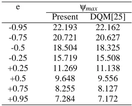
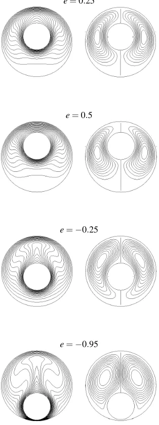
Also, we consider eccentric circular-circular annuli, where the centre of an inner cylinder lies on the vertical symmetrical axis of an outer cylinder. Different amounts of eccentricity (e), namely−0.95,−0.75,−0.5,−0.25,0.25,0.5,0.75 and 0.95, are employed. Since the flow is symmetric, the stream function on the outer and inner cylinders have the same value and they can be set to zeros. Results concerningψmax together with those
of Shu and Zhu [25] for Ra=104are presented in Table 6. It can be seen that both numerical results are in good agreement. Figure 5 shows the streamlines and isotherms of the flow for
[image:5.595.56.282.430.612.2]Grid Outer cylinder, keqo Inner cylinder, keqi
11×11 1.133 1.046
21×21 1.072 1.069
31×31 1.078 1.077
41×41 1.080 1.079
51×51 1.081 1.080
FDM [10] 1.084 1.081
[image:6.595.358.491.68.175.2]DQM [24] 1.082 1.082
Table 2: Circular cylinders: Convergence of computed average equivalent conductivities with grid refinement for Ra=103.
Grid Outer cylinder, keqo Inner cylinder, keqi
31×31 1.698 1.702
41×41 1.704 1.705
51×51 1.709 1.709
61×61 1.711 1.711
FDM [10] 1.735 1.736
DQM [24] 1.715 1.715
Table 3: Circular cylinders: Convergence of computed average equivalent conductivities with grid refinement for Ra=6×10³.
Grid Outer cylinder, keqo Inner cylinder, keqi
41×41 3.089 3.045
51×51 2.936 2.946
61×61 2.922 2.941
FDM [10] 2.973 3.024
DQM [24] 2.958 2.958
Table 4: Circular cylinders: Convergence of computed average equivalent conductivities with grid refinement for Ra=5×10⁴.
Grid Outer cylinder, keqo Inner cylinder, keqi
41×41 3.465 3.254
51×51 3.241 3.187
61×61 3.167 3.174
FDM [10] 3.226 3.308
Table 5: Circular cylinders: Convergence of computed average equivalent conductivities with grid refinement for Ra=7×10⁴.
e ψmax
Present DQM[25]
-0.95 22.193 22.162
-0.75 20.721 20.627
-0.5 18.504 18.325
-0.25 15.719 15.508
+0.25 11.269 11.138
+0.5 9.648 9.556
+0.75 8.255 8.127
+0.95 7.284 7.172
Table 6: Eccentric circular-circular annuli: Comparison ofψmax
for Ra=104between the present technique and DQM.
e ψmax
Present MQ-DQ[2]
-0.75 23.56 23.52
-0.25 18.68 18.64
+0.25 12.40 12.39
+0.75 10.10 10.09
Table 7: Eccentric square-circular annuli: Comparison ofψmax
for Ra=3×10⁵between the present technique and DQM.
Natural Convection in Eccentric Square-Circular Annuli
Consider the natural convection between a heated inner circular cylinder and a cooled square enclosure with their centres lying on the vertical line (Figure 4). An aspect ratio of L/2R=0.26 (L: the side length of the outer square and R: the radius of the inner circle), Pr=0.71, Ra={5×104,3×105,7×105,106} and e={−0.75,−0.25,0.25,0.75}are considered. Like the previous problem, the values ofψalong the inner and outer boundaries can be taken to be zeros. Calculations are conducted on a uniform Cartesian grid of 41×41.
Values ofψmax are given in Table 7. It can be seen that the
present results agree well with those of Ding and Shu [2]. Other results, namely streamlines and isotherms, are shown in Figure 6, where each plot contains 21 contour lines with their levels varying linearly from the minimum to maximum values. Concluding Remarks
In this article, we present a numerical scheme based on Carte-sian grids and 1D-IRBFNs for the simulation of natural convec-tion in circular-circular and square-circular annuli. The main advantages of the present technique lie in the simplicity of the preprocessing, the ease of implementation and the achievement of high Rayleigh-number solutions. Accurate results are ob-tained using relatively coarse grids. This study further demon-strates the great potential of the RBF technique for solving com-plex fluid-flow problems. Extension of the present technique to the case of unsymmetric annuli is currently carried out, and it will be reported in future work.
Acknowledgements
[image:6.595.357.492.240.303.2]e=0.25
e=0.5
e=−0.25
[image:7.595.92.249.175.593.2]e=−0.95
Figure 5: Eccentric circular-circular cylinders: Contour plots of temperature (left) and stream function (right) for the flow at
Ra=104and four different values of e using a grid of 41×41.
Ra=5×10⁴
Ra=3×10⁵
Ra=7×10⁵
Ra=106
References
[1] de Vahl Davis, G., Natural convection of air in a square cav-ity: a bench mark numerical solution, International Journal
for Numerical Methods in Fluids, 3, 1983, 249–264.
[2] Ding, H. and Shu, C., Simulation of natural convection in eccentric annuli between a square outer cylinder and a cir-cular inner cylinder using local MQ-DQ method,
Interna-tional Journal of Computation and Methodology, 47, 2005,
271–313.
[3] Fasshauer, G.E., Solving partial differential equations by collocation with radial basis functions, in Surface Fitting
and Multiresolution Methods, editors A. Le Mehaute, C.
Rabut and L.L., Schumaker, Nashville, TN, Vanderbilt Uni-versity Press, 1997, 131–138.
[4] Glakpe, E.K., Watkins, C.B. and Cannon, J.N., Constant heat flux solutions for natural convection between con-centric and eccon-centric horizontal cylinders, Numerical Heat
Transfer, 10, 1986, 279–295.
[5] Hribersek, M. and Skerget, L., Fast boundary-domain inte-gral algorithm for the computation of incompressible fluid flow problems, International Journal for Numerical
Meth-ods in Fluids, 31, 1999, 891–907.
[6] Kaminski, D.A. and Prakash, C., Conjugate natural convec-tion in a square enclosure: effect of conducconvec-tion in one of the vertical walls, International Journal for Heat and Mass
Transfer, 29(12), 1986, 1979–1988.
[7] Kansa, E.J., Multiquadrics- A scattered data approximation scheme with applications to computational fluid-dynamics-II. Solutions to parabolic, hyperbolic and elliptic partial dif-ferential equations, Computers and Mathematics with
Ap-plications, 19(8/9), 1990, 147–161.
[8] Kansa, E.J. and Hon, Y.C., Circumventing the ill-conditioning problem with multiquadric radial basis func-tions: applications to elliptic partial differential equations,
Computers and Mathematics with Applications, 39, 2000,
123–137.
[9] Kitagawa, K., Wrobel, L.C., Brebbia, C.A. and Tanaka, M., A boundary element formulation for natural convection problems, International Journal for Numerical Methods in
Fluids, 8, 1988, 139–149.
[10] Kuehn, T.H. and Goldstein, R.J., An experimental and theoretical study of natural convection in the annulus be-tween horizontal concentric cylinders, Journal of Fluid
Me-chanics, 74(4), 1976, 695–719.
[11] Le Quere, P., Accurate solutions to the square thermally driven cavity at high Rayleigh number, Computers &
Flu-ids, 20(1), 1991, 29–41.
[12] Madych, W.R. and Nelson, S.A., Multivariate in-terpolation and conditionally positive definite functions, II,Mathematics of Computation, 54(189), 1990, 211–230. [13] Mai-Duy, N. and Tran-Cong, T., Numerical solution of
differential equations using multiquadric radial basis func-tion networks, Neural Networks, 14(2), 2001, 185–199. [14] Mai-Duy, N. and Tran-Cong, T., Numerical solution
of Navier-Stokes equations using multiquadric radial ba-sis function networks,International Journal for Numerical
Methods in Fluids, 37, 2001, 65–86.
[15] Mai-Duy, N. and Tran-Cong, T., Approximation of func-tion and its derivatives using radial basis funcfunc-tion networks,
Applied Mathematical Modelling, 27, 2003, 197–220.
[16] Mai-Duy, N. and Tran-Cong, T., A Cartesian-grid collo-cation method based on radial-basis-function networks for solving PDEs in irregular domains, Numerical Methods for
Partial Differential Equations,23(5), 2007, 1192–1210.
[17] Manzari, M.T., An explicit finite element algorithm for convection heat transfer problems, International Journal of
Numerical Methods for Heat and Fluid Flow, 9(8), 1999,
860–877.
[18] Moukalled, F. and Acharya, S., Natural convection in the annulus between concentric horizontal circular and square cylinders, Journal of Thermophysics and Heat Transfer, 10(3), 1996, 524–531.
[19] Ostrach, S., Natural convection in enclosures, Journal of
Heat Transfer, 110, 1988, 1175–1190.
[20] Power, H. and Mingo, R., The DRM sub-domain decom-position approach for two-dimensional thermal convection flow problems, Engineering Analysis with Boundary
Ele-ments, 24, 2000, 121–127.
[21] Roache, P.J., Computational Fluid Dynamics, Albu-querque, Hermosa Publishers, 1980.
[22] Sammouda, H., Belghith, A. and Surry, C., Finite element simulation of transient natural convection of low-Prandtl-number fluids in heated cavity, International Journal of
Nu-merical Methods for Heat and Fluid Flow, 9(5), 1999, 612–
624.
[23] Sarler, B., A radial basis function collocation approach in computational fluid dynamics, Computer Modeling in
En-gineering and Sciences, 7(2), 2005, 185–194.
[24] Shu, C., Application of differential quadrature method to simulate natural convection in a concentric annulus,
In-ternational Journal for Numerical Methods in Fluids, 30,
1999, 977–993.
[25] Shu, C. and Zhu, Y.D., Numerical analysis of flow and thermal field in arbitrary eccentric annulus by differential quadrature method, Journal for Heat and Mass transfer, 38, 2001, 597–608.
[26] Shu, C. and Zhu, Y.D., Efficient computation of natural convection in a concentric annulus between an outer square cylinder and an inner circular cylinder, International
Jour-nal for Numerical Methods in Fluids, 38, 2002, 429–445.
[27] Zerroukat, T., Power, H. and Chen, C.S., A numerical method for heat transfer problems using collocation and ra-dial basis functions, International Journal for Numerical