DATA STREAMS USING PROJECTED OUTLIER ANALYSIS
STRATEGY
by
Ji Zhang
Submitted in partial fulfillment of the requirements for the degree of Doctor of Philosophy
at
Dalhousie University Halifax, Nova Scotia
December 2008
c
FACULTY OF COMPUTER SCIENCE
The undersigned hereby certify that they have read and recommend to the Faculty of Graduate Studies for acceptance a thesis entitled “TOWARDS OUTLIER DETECTION FOR HIGH-DIMENSIONAL DATA STREAMS USING PROJECTED OUTLIER ANALYSIS STRATEGY” by Ji Zhang in partial fulfillment of the requirements for the degree of Doctor of Philosophy.
Dated: December 10, 2008
External Examiner:
Research Supervisor:
Examining Committee:
DATE: December 10, 2008 AUTHOR: Ji Zhang
TITLE: TOWARDS OUTLIER DETECTION FOR HIGH-DIMENSIONAL DATA STREAMS USING PROJECTED OUTLIER ANALYSIS STRATEGY
DEPARTMENT OR SCHOOL: Faculty of Computer Science
DEGREE: PhD CONVOCATION: May YEAR: 2009
Permission is herewith granted to Dalhousie University to circulate and to have copied for non-commercial purposes, at its discretion, the above title upon the request of individuals or institutions.
Signature of Author
The author reserves other publication rights, and neither the thesis nor extensive extracts from it may be printed or otherwise reproduced without the author’s written permission.
The author attests that permission has been obtained for the use of any copyrighted material appearing in the thesis (other than brief excerpts requiring only proper acknowledgement in scholarly writing) and that all such use is clearly acknowledged.
List of Tables . . . vii
List of Figures . . . viii
Abstract . . . xi
List of Abbreviations Used . . . xii
Acknowledgements . . . xiii
Chapter 1 Introduction . . . 1
Chapter 2 Related Work . . . 6
2.1 Scope of the Review . . . 6
2.2 Outlier Detection Methods for Low Dimensional Data . . . 9
2.2.1 Statistical Detection Methods . . . 9
2.2.2 Distance-based Methods . . . 16
2.2.3 Density-based Methods . . . 27
2.2.4 Clustering-based Methods . . . 33
2.3 Outlier Detection Methods for High Dimensional Data . . . 40
2.3.1 Methods for Detecting Outliers in High-dimensional Data . . . 40
2.3.2 Outlying Subspace Detection for High-dimensional Data . . . 44
2.3.3 Clustering Algorithms for High-dimensional Data . . . 47
2.4 Outlier Detection Methods for Data Streams . . . 49
2.5 Summary . . . 53
Chapter 3 Concepts and Definitions . . . 56
3.1 Time Model and Decaying Function . . . 56
3.2.2 Inverse Relative Standard Deviation (IRSD) . . . 61
3.2.3 Inverse k-Relative Distance (IkRD) . . . 61
3.3 Definition of Projected Outliers . . . 62
3.4 Computing PCS of a Projected Cell . . . 63
3.4.1 Computing Density of a Projected Cell Dc . . . 64
3.4.2 Computing Mean of a Projected Cell µc . . . 64
3.4.3 Computing Standard Deviation of a Projected Cell σc . . . 65
3.4.4 Generate Representative Data Points in a Subspace . . . 65
3.5 Maintaining the PCS of a Projected Cell . . . 66
3.5.1 Update RD of the PCS . . . 67
3.5.2 Update IRSD of the PCS . . . 68
3.5.3 Update Representative Points in a Subspace . . . 69
3.6 Summary . . . 72
Chapter 4 SPOT: Stream Projected Outlier Detector . . . 73
4.1 An Overview of SPOT . . . 73
4.2 Learning Stage of SPOT . . . 74
4.3 Detection Stage of SPOT . . . 81
4.4 Summary . . . 85
Chapter 5 Multi-Objective Genetic Algorithm . . . 86
5.1 An Overview of Evolutionary Multiobjective Optimization . . . 86
5.1.1 Multiobjective Optimization Problem Formulation . . . 87
5.1.2 Major Components of Evolutionary Algorithms . . . 89
5.1.3 Important Issues of MOEAs . . . 90
5.2 Design of MOEA in SPOT . . . 95
5.3 Objective Functions . . . 95
5.3.1 Definition of Objective Functions . . . 95
5.4 Selection Operators . . . 99
5.5 Search Operators . . . 99
5.6 Individual Representation . . . 100
5.7 Elitism . . . 104
5.8 Diversity Preservation . . . 105
5.9 Algorithm of MOGA . . . 106
5.10 Summary . . . 107
Chapter 6 Performance Evaluation . . . 108
6.1 Data Preparation and Interface Development . . . 108
6.1.1 Synthetic Data Sets . . . 108
6.1.2 Real-life Data Sets . . . 109
6.2 Experimental Results . . . 140
6.2.1 Scalability Study of SPOT . . . 140
6.2.2 Convergence and Adaptability Study of SPOT . . . 144
6.2.3 Sensitivity Study of SPOT . . . 147
6.2.4 Effectiveness Study of SPOT . . . 151
6.3 Summary . . . 176
Chapter 7 Conclusions . . . 179
7.1 Research Summary . . . 179
7.2 Limitations of SPOT . . . 181
7.3 Future Research . . . 182
7.3.1 Adaptation of SST . . . 182
7.3.2 Optimization of Partition Size δ . . . 182
7.3.3 Distributed Outlier Detection Using SPOT . . . 183
Bibliography . . . 184
Table 5.1 Crossover Lookup Table (identif ier = 1, L= 2) . . . 102
Table 6.1 List of anonymized attributes . . . 111
Table 6.2 List of attributes used in anomaly detection . . . 112
Table 6.3 Temporal contexts for data partitioning . . . 113
Table 6.4 SC results of different validation method candidates . . . 121
Table 6.5 The time-decayed signature subspace lookup table . . . 134
Table 6.6 Performance of SPOT under varying thresholds . . . 148
Table 6.7 Comparison of different methods using SD2 . . . 156
Table 6.8 Anomaly detection analysis for different temporal contexts . . . 168
Table 6.9 Percentage of the anomalies that have redundant outlying sub-spaces . . . 170
Table 6.10 Redundancy Ratio of different data sets . . . 171
Table 6.11 Comparison of the manual and automatic methods for identify-ing false positives . . . 172
Table 6.12 Comparing SPOT and the winning entry of KDD CUP’99 . . . 176
Table 6.13 Performance rank of different methods for data streams gener-ated by SD2 . . . 177
Table 6.14 Performance rank of different methods for KDD-CUP’99 data stream . . . 177
Table 6.15 Performance rank of different methods for wireless network data stream . . . 178
Figure 2.1 Points with the same Dk value but different outlier-ness . . . . 22
Figure 2.2 Local and global perspectives of outlier-ness of p1 and p2 . . . 25
Figure 2.3 A sample dataset showing the advantage of LOF overDB(k, λ )-Outlier . . . 28
Figure 2.4 An example where LOF does not work . . . 31
Figure 2.5 Definition of MDEF . . . 32
Figure 2.6 A summary of major existing outlier detection methods . . . . 55
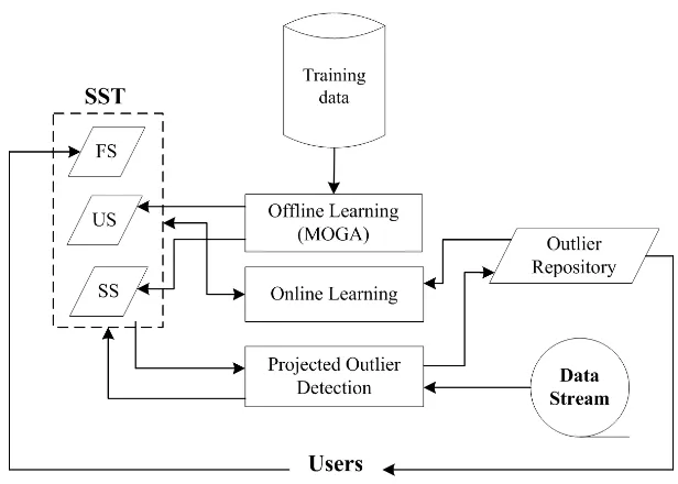
Figure 4.1 An overview of SPOT . . . 74
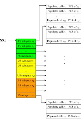
Figure 4.2 The data structure of SST . . . 79
Figure 4.3 Unsupervised learning algorithm of SPOT . . . 80
Figure 4.4 Supervised learning algorithm of SPOT . . . 80
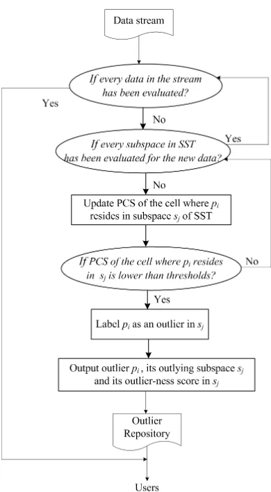
Figure 4.5 The steps of detection stage in SPOT . . . 82
Figure 4.6 Detecting algorithm of SPOT . . . 84
Figure 5.1 An crossover example of two integer strings (withϕ = 8,L= 2, lc = 3) . . . 103
Figure 5.2 Algorithm of MOGA . . . 106
Figure 6.1 Using centroid and representative points to measure outlier-ness of data points . . . 116
Figure 6.2 Cluster representative points generation . . . 117
Figure 6.3 Generating single training data set for obtaining SS . . . 128
Figure 6.4 Generating multiple training data sets for obtaining SS . . . . 128
Figure 6.5 Example of outlying subspaces and its corresponding Outlying Subspace Front (OSF) for an anomaly . . . 130
positive class . . . 139
Figure 6.8 Scalability of learning process w.r.t data number . . . 141
Figure 6.9 Scalability of learning process w.r.t data dimension . . . 142
Figure 6.10 Scalability of detection process w.r.t data number . . . 143
Figure 6.11 Scalability of detection process w.r.t data dimension . . . 144
Figure 6.12 Throughput analysis of SPOT . . . 145
Figure 6.13 Convergence study of MOGA . . . 146
Figure 6.14 Evolution of SST . . . 147
Figure 6.15 Effect of search workload on speed of MOGA . . . 148
Figure 6.16 Effect of search workload on objective optimization . . . 150
Figure 6.17 Effect of number of clustering iterations . . . 151
Figure 6.18 Effect of number of top outlying training data selected . . . . 152
Figure 6.19 Precision, recall and F-measure of SPOT and the histogram based method . . . 157
Figure 6.20 Precision, recall andF-measure of SPOT and the Kernel-function based method . . . 158
Figure 6.21 Precision, recall and F-measure of SPOT and the Incremental LOF . . . 159
Figure 6.22 Efficiency comparison of SPOT and Incremental LOF . . . 160
Figure 6.23 Percentage of true anomalies detected by SPOT, the Kernel function-based detection method and Incremental LOF under varying search workloads . . . 161
Figure 6.24 Precision, recall and F-measure of SPOT and HPStream . . . 162
Figure 6.25 Precision and recall of HPStream under a varying number of clusters . . . 163
Figure 6.26 Precision, recall andF-measure of SPOT and the Largest-Cluster detection method . . . 165
tion method . . . 166 Figure 6.28 F-measure of SPOT and the Largest-Cluster detection method
under varying number of validation subspaces . . . 167 Figure 6.29 Effect of number of training data sets for each attack class . . 169 Figure 6.30 Number of strong signature subspaces for each attack class
un-der varying number of data being processed . . . 173 Figure 6.31 ROC curves of different methods . . . 174
Outlier detection is an important research problem in data mining that aims to dis-cover useful abnormal and irregular patterns hidden in large data sets. Most existing outlier detection methods only deal with static data with relatively low dimensionality. Recently, outlier detection for high-dimensional stream data became a new emerging research problem. A key observation that motivates this research is that outliers in high-dimensional data are projected outliers, i.e., they are embedded in lower-dimensional subspaces. Detecting projected outliers from high-lower-dimensional stream data is a very challenging task for several reasons. First, detecting projected outliers is difficult even for high-dimensional static data. The exhaustive search for the out-lying subspaces where projected outliers are embedded is a NP problem. Second, the algorithms for handling data streams are constrained to take only one pass to pro-cess the streaming data with the conditions of space limitation and time criticality. The currently existing methods for outlier detection are found to be ineffective for detecting projected outliers in high-dimensional data streams.
In this thesis, we present a new technique, called the Stream Project Outlier deTector (SPOT), which attempts to detect projected outliers in high-dimensional data streams. SPOT employs an innovative window-based time model in capturing dynamic statistics from stream data, and a novel data structure containing a set of top sparse subspaces to detect projected outliers effectively. SPOT also employs a multi-objective genetic algorithm as an effective search method for finding the outlying subspaces where most projected outliers are embedded. The experimental results demonstrate that SPOT is efficient and effective in detecting projected outliers for high-dimensional data streams. The main contribution of this thesis is that it provides a backbone in tackling the challenging problem of outlier detection for high-dimensional data streams. SPOT can facilitate the discovery of useful abnormal patterns and can be potentially applied to a variety of high demand applications, such as for sensor network data monitoring, online transaction protection, etc.
SPOT: Stream Projected Outlier Detector
SST: Sparse Subspace Template
FS: Fixed Subspaces
US: Unsupervised Subspaces
SS: Supervised Subspaces
BCS: Base Cell Summary
PCS: Projected Cell Summary
RD: Relative Density
IRSD: Inverse Relative Standard Deviation
IkRD: Inverse k-Relative Distance
MOGA: Multiobjective Genetic Algorithm
CLT: Crossover Lookup Table
MTPT: Mutation Transition Probability Table
MSE: Mean Square Error
SC: Silhouette Coefficient
ROC: Receiver Operating Characteristic
First and foremost, I would like to thank my supervisor Dr. Qigang Gao and Dr. Hai Wang for their dedicated supervision during my Ph.D study. Their endless help, care, kindness, patience, generosity, and thoughtful considerations are greatly valued. I would like to thank Dr. Malcolm Heywood for his wonderful course on Genetic Algorithms. It is his course that has stimulated much of my interest in this area, which greatly contributes to my Ph.D research.
I greatly appreciate Dr. John McHugh for his willingness to share his wide scope of knowledge with me and to give valuable suggestions on some parts of my Ph.D research.
I would also like to thank Dr. Christian Blouin for his interesting course in Bioinformatics. I learned much from this course that paved a good foundation for my long-term research career development.
I would like to thank Killam Trust as well for awarding me the prestigious Kil-lam Predoctoral Scholarship, which provides a strong financial support to my Ph.D research activities. I deeply appreciate Dr. Qigang Gao, Dr. Hai Wang and Dr. Mal-colm Heywood for their unreserved support in my application for this scholarship.
Thanks also go to the faculty of Computer Science for the good research facility and atmosphere it created. In particular, I am very grateful to the personal help from Dr. Srinivas Sampalli and Ms. Menen Teferra for many times.
I would like to thank my all colleagues and friends for the good time we have had in Dalhousie. I would like to thank my family for their continued support and care. It would be impossible to finish my Ph.D study without their continuous understanding and support.
Introduction
Outlier detection is an important research problem in data mining that aims to find objects that are considerably dissimilar, exceptional and inconsistent with respect to the majority data in an input database [60]. In recent years, we have witnessed a tremendous research interest sparked by the explosion of data collected and trans-ferred in the format of streams. This poses new opportunities as well as challenges for research efforts in outlier detection. A data stream is a real-time, continuous and ordered (implicitly by arrival sequence or explicitly by timestamp) sequence of items. Examples of data streams include network traffic, telecommunications data, financial market data, data from sensors that monitor the weather and environment, surveillance video and so on. Outlier detection from stream data can find items (ob-jects or points) that are abnormal or irregular with respect to the majority of items in the whole or a horizon/window of the stream. Outlier detection in data streams can be useful in many fields such as analysis and monitoring of network traffic data (e.g., connection-oriented records), web log, wireless sensor networks and financial transactions, etc.
A key observation that motivates this research is that outliers existing in high-dimensional data streams are embedded in some lower-high-dimensional subspaces. Here, a subspace refers to as the data space consisting of a subset of attributes. These outliers are termed projected outliers in the high-dimensional space. The existence of projected outliers is due to the fact that, as the dimensionality of data goes up, data tend to become equally distant from each other. As a result, the difference of data points’ outlier-ness will become increasingly weak and thus undistinguishable. Only in moderate or low dimensional subspaces can significant outlier-ness of data be observed. This phenomena is commonly referred to as thecurse of dimensionality
[17]. Because most of state-of-the-art outlier detection methods perform detection in the full data space, thus the projected outliers cannot be found by these methods. This will lead to a loss of interesting and potentially useful abnormal patterns hidden in high-dimensional data streams.
In this research, we will study the problem of detecting projected outliers from high-dimensional data streams. This problem can be formulated as follows: given a data stream D with a potentially unbounded size of ϕ-dimensional data points, for each data point pi = {pi1, pi2, . . . , piϕ} in D, projected outlier detection method performs a mapping as
f :pi →(b, Si, Scorei)
where each data pi is mapped to a triplet (b, Si, Scorei). b is a Boolean variable indicating whether or not pi is a projected outlier. If pi is a projected outlier (i.e.,
b=true), thenSi is the set of outlying subspaces ofpiandScoreiis the corresponding outlier-ness score of pi in each subspace of Si. In the case that pi is a normal data, we have b =f alse, Si =∅and Scorei is not applicable.
The results of the detection method will be a set of projected outliers and their associated outlying subspace(s) and outlier-ness score to characterize the context and strength of the projected outliers detected. The results, denoted byA, can be formally expressed as
A={< o, S, Score >,o∈O}
whereO denotes the set of projected outliers detected. The users have the discretion to pick up the top k projected outliers that have the highest outlier-ness from O. In contrast, the traditional definition of outliers does not explicitly present outlying subspaces of outliers in the final result as outliers are detected in the full or a pre-specified data space that is known to users before outliers are detected.
1. First, finding the right outlying subspaces for projected outliers is crucial to de-tection performance of the algorithm. Once these outlying subspaces have been found, detecting projected outliers in these subspace will then become a much easier task. Nevertheless, the number of possible subspaces increases dramati-cally with the data dimensionality. Thus, finding the outlying subspaces of the data through an exhaustive search of the space lattice is rather computationally demanding and totally infeasible when the dimensionality of data is high. In light of this, the outlier detection algorithm should be reasonably efficient to find the right subspaces in which projected outliers can be accurately detected; 2. Another aspect of the challenge originates from the characteristics of stream-ing data themselves. First, data streams can only be accessed in the order of their arrivals and random access is disallowed. Second, data streams are potentially unbound in size and the space available to store information is sup-posed to be small. Finally, data objects in the stream usually have implicit or explicit time concept (e.g., timestamps). Because of these unique features of data streams, data stream outlier detection algorithms can only have one pass over data streams and process data in an incremental, online and real-time paradigm. In addition, they should feature constant and short time for process-ing each data object and limited space for storprocess-ing information. They need to employ dynamic and space-economic data synopsis that can be updated incre-mentally and efficiently. Finally, they are expected to take into account the time concept in the detection process. They should apply appropriate time model(s) to discriminate data arriving at different time, and have necessary capability to cope with concept drift that may occur in the streams.
only applicable to relatively low dimensional static data [26][76][77][101][111]. Be-cause they use the full set of attributes for outlier detection, thus they are not able to detect projected outliers. They cannot handle data streams either. Recently, there are some emerging work in dealing with outlier detection either in high-dimensional static data or data streams. However, there has not been any reported concrete research work so far for exploring the intersection of these two active research di-rections. For those methods in projected outlier detection in high-dimensional space [14][123][131][126][128], they can detect projected outliers that are embedded in sub-spaces. However, their measurements used for evaluating points’ outlier-ness are not incrementally updatable and many of the methods involve multiple scans of data, making them incapable of handling data streams. For instance, [14][123] use the Sparsity Coefficient to measure data sparsity. Sparsity Coefficient is based on an equi-depth data partition that has to be updated frequently from the data stream. This will be expensive and such updates will require multiple scans of data. [131][126][128] use data sparsity metrics that are based on distance involving the concept of k near-est neighbors (kNN). This is not suitable for data streams either as one scan of data is not sufficient for retaining kNN information of data points. One the other hand, the techniques for tackling outlier detection in data streams [100][1] rely on full data space to detect outliers and thus projected outliers cannot be discovered by these techniques. As such, it is desirable to propose a new method that well solves the drawbacks of these existing methods.
In this thesis, we present a new technique, called Stream Projected Outlier deTec-tor (SPOT), to approach the problem of outlier detection in high-dimensional data streams. The major contributions of this research can be summarized as follows:
• SPOT constructs a Sparse Subspace Template (SST) to detect projected out-liers. SST consists of a number of mutually supplemented subspace groups that contribute collectively to an effective detection of projected outliers. SPOT is able to perform supervised and/or unsupervised learning to construct SST, providing a maximum level of flexibility to users. Self-evolution of SST has also been incorporated into SPOT to greatly enhance its adaptability to dynamics of data streams;
• Unlike most of other outlier detection methods that measure outlier-ness of data points based on a single criterion, SPOT adopts a more flexible framework of using multiple measurements for this purpose. SPOT utilizes the Multi-Objective Genetic Algorithm (MOGA) as an effective search method to find subspaces that are able to optimize all the criteria for constructing SST; • Last but not the least, we show that SPOT is efficient and effective in detecting
projected outliers in subspaces and outperforms the major existing methods through experiments on both synthetic and real-life data streams.
Roadmap
Related Work
We have witnessed considerable research efforts in outlier detection in the past a few years. This section presents a review on the major state-of-the-art outlier detection methods. To facilitate a systematic survey of the existing outlier detection methods, the scope of this review is first clearly specified. The organization of the literature review is as follows. We will first review the conventional outlier detection techniques that are primarily suitable for relatively low-dimensional static data, followed by some of recent advancements in outlier detection for high-dimensional static data and data streams.
2.1 Scope of the Review
Before the review of outlier detection methods is presented, it is necessary for us to first explicitly specify the scope of this review. There have been a lot of research work in detecting different kinds of outliers from various types of data where the techniques outlier detection methods utilize differ considerably. Most of the existing outlier detection methods detect the so-calledpoint outliers from vector-like data sets. This is the focus of this review as well as of this thesis. Another common category of outliers that has been investigated is called collective outliers. Besides the vector-like data, outliers can also be detected from other types of data such as sequences, trajectories and graphs, etc. In the reminder of this subsection, we will discuss briefly different types of outliers.
First, outliers can be classified as point outliers and collective outliers based on the number of data instances involved in the concept of outliers.
• Point outliers. In a given set of data instances, an individual outlying instance is termed as a point outlier. This is the simplest type of outliers and is the focus
of majority of existing outlier detection schemes [33]. A data point is detected as a point outlier because it displays outlier-ness at its own right, rather than together with other data points. In most cases, data are represented in vectors as in the relational databases. Each tuple contains a specific number of attributes. The principled method for detecting point outliers from vector-type data sets is to quantify, through some outlier-ness metrics, the extent to which each single data is deviated from the other data in the data set.
• Collective outliers. A collective outlier represents a collection of data in-stances that is outlying with respect to the entire data set. The individual data instance in a collective outlier may not be outlier by itself, but the joint occurrence as a collection is anomalous [33]. Usually, the data instances in a collective outlier are related to each other. A typical type of collective outliers are sequence outliers, where the data are in the format of an ordered sequence.
Outliers can also be categorized into vector outliers, sequence outliers, trajectory outliers and graph outliers, etc, depending on the types of data from where outliers can be detected.
• Vector outliers. Vector outliers are detected from vector-like representation of data such as the relational databases. The data are presented in tuples and each tuple has a set of associated attributes. The data set can contain only numeric attributes, or categorical attributes or both. Based on the number of attributes, the data set can be broadly classified as low-dimensional data and high-dimensional data, even though there is not a clear cutoff between these two types of data sets. As relational databases still represent the mainstream approaches for data storage, therefore, vector outliers are the most common type of outliers we are dealing with.
of commands in this log may look like the following sequence: http-web, buffer-overflow, http-web, http-web, smtp-mail, ftp, http-web, ssh. Outlying sequence of commands may indicate a malicious behavior that potentially compromises system security. In order to detect abnormal command sequences, normal com-mand sequences are maintained and those sequences that do not match any normal sequences are labeled sequence outliers. Sequence outliers are a form of collective outlier.
• Trajectory outliers. Recent improvements in satellites and tracking facilities have made it possible to collect a huge amount of trajectory data of moving objects. Examples include vehicle positioning data, hurricane tracking data, and animal movement data [83]. Unlike a vector or a sequence, a trajectory is typically represented by a set of key features for its movement, including the coordinates of the starting and ending points; the average, minimum, and maximum values of the directional vector; and the average, minimum, and maximum velocities. Based on this representation, a weighted-sum distance function can be defined to compute the difference of trajectory based on the key features for the trajectory [78]. A more recent work proposed a partition-and-detect framework for partition-and-detecting trajectory outliers [83]. The idea of this method is that it partitions the whole trajectory into line segments and tries to detect outlying line segments, rather than the whole trajectory. Trajectory outliers can be point outliers if we consider each single trajectory as the basic data unit in the outlier detection. However, if the moving objects in the trajectory are considered, then an abnormal sequence of such moving objects (constituting the sub-trajectory) is a collective outlier.
substructure in the graph [90]. Graph outliers can be either point outliers (e.g., node and edge outliers) or collective outliers (e.g., sub-graph outliers).
Unless otherwise stated, all the outlier detection methods discussed in this review refer to those methods for detecting point outliers from vector-like data sets.
2.2 Outlier Detection Methods for Low Dimensional Data
The earlier research work in outlier detection mainly deals with static datasets with relatively low dimensions. Literature on these work can be broadly classified into four major categories based on the techniques they used, i.e., statistical methods, distance-based methods, density-based methods and clustering-based methods.
2.2.1 Statistical Detection Methods
Statistical outlier detection methods [28, 57] rely on the statistical approaches that assume a distribution or probability model to fit the given dataset. Under the dis-tribution assumed to fit the dataset, the outliers are those points that do not agree with or conform to the underlying model of the data.
The statistical outlier detection methods can be broadly classified into two cat-egories, i.e., the parametric methods and the non-parametric methods. The major differences between these two classes of methods lie in that the parametric methods assume the underlying distribution of the given data and estimate the parameters of the distribution model from the given data [41] while the non-parametric methods do not assume any knowledge of distribution characteristics [38].
Statistical outlier detection methods (parametric and non-parametric) typically take two stages for detecting outliers,i.e., the training stage and test stage.
normal instances, or outliers, depending on the availability of labels. Unsuper-vised techniques determine a statistical model or profile which fits all or the majority of the instances in the given data set;
• Test stage. Once the probabilistic model or profile is constructed, the next step is to determine if a given data instance is an outlier with respect to the model/profile or not. This involves computing the posterior probability of the test instance to be generated by the constructed model or the deviation from the constructed data profile. For example, we can find the distance of the data instance from the estimated mean and declare any point above a threshold to be an outlier [51].
Parametric Methods
Parametric statistical outlier detection methods explicitly assume the probabilistic or distribution model(s) for the given data set. Model parameters can be estimated using the training data based upon the distribution assumption. The major parametric outlier detection methods include Gaussian model-based and regression model-based methods.
A. Gaussian Models
In the mean-variance test for a Gaussian distribution N(µ, σ2), where the population
has a mean µ and variance σ, outliers can be considered to be points that lie 3 or more standard deviations (i.e., ≥3σ) away from the mean [50]. This test is general and can be applied to some other commonly used distributions such as Student t -distribution and Poisson -distribution, which feature a fatter tail and a longer right tail than a normal distribution, respectively. The box-plot test draws on the box plot to graphically depict the distribution of data using five major attributes, i.e., smallest non-outlier observation (min), lower quartile (Q1), median, upper quartile (Q3), and largest non-outlier observation (max). The quantity Q3-Q1 is called the Inter Quartile Range (IQR). IQR provides a means to indicate the boundary beyond which the data will be labeled as outliers; a data instance will be labeled as an outlier if it is located 1.5*IQR times lower than Q1 or 1.5*IQR times higher than Q3.
In some cases, a mixture of probabilistic models may be used if a single model is not sufficient for the purpose of data modeling. If labeled data are available, two separate models can be constructed, one for the normal data and another for the outliers. The membership probability of the new instances can be quantified and they are labeled as outliers if their membership probability of outlier probability model is higher than that of the model of the normal data. The mixture of probabilistic models can also be applied to unlabeled data, that is, the whole training data are modeled using a mixture of models. A test instance is considered to be an outlier if it is found that it does not belong to any of the constructed models.
B. Regression Models
specifically, such test involves comparing the actual instance value and its projected value produced by the regression model. A data point is labeled as an outlier if a re-markable deviation occurs between the actual value and its expected value produced by the regression model.
Basically speaking, there are two ways to use the data in the dataset for building the regression model for outlier detection, namely thereverse search anddirect search methods. The reverse search method constructs the regression model by using all data available and then the data with the greatest error are considered as outliers and excluded from the model. The direct search approach constructs a model based on a portion of data and then adds new data points incrementally when the preliminary model construction has been finished. Then, the model is extended by adding most fitting data, which are those objects in the rest of the population that have the least deviations from the model constructed thus far. The data added to the model in the last round, considered to be the least fitting data, are regarded to be outliers.
Non-parametric Methods
The outlier detection techniques in this category do not make any assumptions about the statistical distribution of the data. The most popular approaches for outlier detection in this category are histograms and Kernel density function methods.
A. Histograms
The most popular non-parametric statistical technique is to use histograms to maintain a profile of data. Histogram techniques by nature are based on the frequency or counting of data.
The histogram based outlier detection approach is typically applied when the data has a single feature. Mathematically, a histogram for a feature of data consists of a number of disjoint bins (or buckets) and the data are mapped into one (and only one) bin. Represented graphically by the histogram graph, the height of bins corresponds to the number of observations that fall into the bins. Thus, if we let n be the total number of instances,k be the total number of bins andmibe the number of data point in theithbin (1≤i≤k), the histogram satisfies the following conditionn =Pk
The training stage involves building histograms based on the different values taken by that feature in the training data.
The histogram techniques typically define a measure between a new test instance and the histogram based profile to determine if it is an outlier or not. The measure is defined based on how the histogram is constructed in the first place. Specifically, there are three possible ways for building a histogram:
1. The histogram can be constructed only based on normal data. In this case, the histogram only represents the profile for normal data. The test stage evaluates whether the feature value in the test instance falls in any of the populated bins of the constructed histogram. If not, the test instance is labeled as an outlier [5] [68][58];
2. The histogram can be constructed only based on outliers. As such, the his-togram captures the profile for outliers. A test instance that falls into one of the populated bins is labeled as an outlier [39]. Such techniques are particularly popular in intrusion detection community [41][45] [35] and fraud detection [49]; 3. The histogram can be constructed based on a mixture of normal data and outliers. This is the typical case where histogram is constructed. Since normal data typically dominate the whole data set, thus the histogram represents an approximated profile of normal data. The sparsity of a bin in the histogram can be defined as the ratio of frequency of this bin against the average frequency of all the bins in the histogram. A bin is considered as sparse if such ratio is lower than a user-specified threshold. All the data instance falling into the sparse bins are labeled as outliers.
The first and second ways for constructing histogram, as presented above, rely on the availability of labeled instances, while the third one does not.
likelihoods for calculating outlier score is typically done using the following equation:
Outlier Score =X
f∈F
wf ·(1−pf)/|F|
wherewf denotes the weight assigned for feature f,pf denotes the probability for the value of feature f and F denotes the set of features of the dataset. Such histogram-based aggregation techniques have been used in intrusion detection in system call data [42], fraud detection [49], damage detection in structures [85] [88] [89], network intru-sion detection [115] [117], web-based attack detection [81], Packet Header Anomaly Detection (PHAD), Application Layer Anomaly Detection (ALAD) [87], NIDES (by SRI International) [5] [12] [99]. Also, a substantial amount of research has been done in the field of outlier detection for sequential data (primarily to detect intrusions in computer system call data) using histogram based techniques. These techniques are fundamentally similar to the instance based histogram approaches as described above but are applied to sequential data to detect collective outliers.
Histogram based detection methods are simple to implement and hence are quite popular in domain such as intrusion detection. But one key shortcoming of such techniques for multivariate data is that they are not able to capture the interactions between different attributes. An outlier might have attribute values that are individ-ually very frequent, but their combination is very rare. This shortcoming will become more salient when dimensionality of data is high. A feature-wise histogram technique will not be able to detect such kinds of outliers. Another challenge for such techniques is that users need to determine an optimal size of the bins to construct the histogram.
B. Kernel Functions
Another popular non-parametric approach for outlier detection is the parzen win-dows estimation due to Parzen [94]. This involves using Kernel functions to approxi-mate the actual density distribution. A new instance which lies in the low probability area of this density is declared to be an outlier.
density function (pdf ) is
fh(x) = 1
Nh
N
X
i=1
K(x−xi
h )
where K is Kernel function and h is the bandwidth (smoothing parameter). Quite often, K is taken to be a standard Gaussian function with mean µ= 0 and variance
σ2 = 1:
K(x) = √1 2πe
−12x2
Novelty detection using Kernel function is presented by [19] for detecting novelties in oil flow data. A test instance is declared to be novel if it belongs to the low density area of the learnt density function. Similar application of parzen windows is proposed for network intrusion detection [34] and for mammographic image analysis [110]. A semi-supervised probabilistic approach is proposed to detect novelties [38]. Kernel functions are used to estimate the probability distribution function (pdf) for the normal instances. Recently, Kernel functions are used in outlier detection in sensor networks [100][30].
Kernel density estimation of pdf is applicable to both univariate and multivariate data. However, the pdf estimation for multivariate data is much more computation-ally expensive than the univariate data. This renders the Kernel density estimation methods rather inefficient in outlier detection for high-dimensional data.
Advantages and Disadvantages of Statistical Methods
Statistical outlier detection methods feature some advantages. They are mathemati-cally justified and if a probabilistic model is given, the methods are very efficient and it is possible to reveal the meaning of the outliers found [93]. In addition, the model constructed, often presented in a compact form, makes it possible to detect outliers without storing the original datasets that are usually of large sizes.
the univariate feature space. Thus, they are unsuitable even for moderate multi-dimensional data sets. This greatly limits their applicability as in most practical applications the data is multiple or even high dimensional. In addition, a lack of the prior knowledge regarding the underlying distribution of the dataset makes the distribution-based methods difficult to use in practical applications. A single distri-bution may not model the entire data because the data may originate from multiple distributions. Finally, the quality of results cannot be guaranteed because they are largely dependent on the distribution chosen to fit the data. It is not guaranteed that the data being examined fit the assumed distribution if there is no estimate of the dis-tribution density based on the empirical data. Constructing such tests for hypothesis verification in complex combinations of distributions is a nontrivial task whatsoever. Even if the model is properly chosen, finding the values of parameters requires com-plex procedures. From above discussion, we can see the statistical methods are rather limited to large real-world databases which typically have many different fields and it is not easy to characterize the multivariate distribution of exemplars.
For non-parametric statistical methods, such as histogram and Kernal function methods, they do not have the problem of distribution assumption that the parametric methods suffer and they both can deal with data streams containing continuously arriving data. However, they are not appropriate for handling high-dimensional data. Histogram methods are effective for a single feature analysis, but they lose much of their effectiveness for multi or high-dimensional data because they lack the ability to analyze multiple feature simultaneously. This prevents them from detecting subspace outliers. Kernel function methods are appropriate only for relatively low dimensional data as well. When the dimensionality of data is high, the density estimation using Kernel functions becomes rather computationally expensive, making it inappropriate for handling high-dimensional data streams.
2.2.2 Distance-based Methods
outlier detection techniques are defined based upon the concepts oflocal neighborhood orknearest neighbors (kNN) of the data points. The notion of distance-based outliers does not assume any underlying data distributions and generalizes many concepts from distribution-based methods. Moreover, distance-based methods scale better to multi-dimensional space and can be computed much more efficiently than the statistical-based methods.
In distance-based methods, distance between data points is needed to be com-puted. We can use any of the Lp metrics like the Manhattan distance or Euclidean distance metrics for measuring the distance between a pair of points. Alternately, for some other application domains with presence of categorical data (e.g., text doc-uments), non-metric distance functions can also be used, making the distance-based definition of outliers very general. Data normalization is normally carried out in order to normalize the different scales of data features before outlier detection is performed.
A. Local Neighborhood Methods
The first notion of distance-based outliers, calledDB(k, λ)-Outlier, is due to Knorr and Ng [76]. It is defined as follows. A point p in a data set is a DB(k, λ)-Outlier, with respect to the parameters k and λ, if no more than k points in the data set are at a distance λ or less (i.e., λ−neighborhood) from p. This definition of outliers is intuitively simple and straightforward. The major disadvantage of this method, however, is its sensitivity to the parameter λ that is difficult to specify a priori. As we know, when the data dimensionality increases, it becomes increasingly difficult to specify an appropriate circular local neighborhood (delimited by λ) for outlier-ness evaluation of each point since most of the points are likely to lie in a thin shell about any point [24]. Thus, a too small λ will cause the algorithm to detect all points as outliers, whereas no point will be detected as outliers if a too large λis picked up. In other words, one needs to choose an appropriateλwith a very high degree of accuracy in order to find a modest number of points that can then be defined as outliers.
pct% of the objects in the datasets have the distance larger than dmin from this ob-ject [77][78]. Similar to DB(k, λ)-Outlier, this method essentially delimits the local neighborhood of data points using the parameter dmin and measures the outlierness of a data point based on the percentage, instead of the absolute number, of data points falling into this specified local neighborhood. As pointed out in [74] and [75],
DB(pct, dmin) is quite general and is able to unify the exisiting statisical detection methods using discordancy tests for outlier detection. For exmaple, DB(pct, dmin) unifies the definition of outliers using a normal distribution-based discordancy test with pct = 0.9988 and dmin = 0.13. The specification of pct is obviously more intuitive and easier than the specification of k in DB(k, λ)-Outliers [77]. However,
DB(pct, dmin)-Outlier suffers a similar problem asDB(pct, dmin)-Outlier in specifying the local neighborhood parameter dmin.
To efficiently calculate the number (or percentage) of data points falling into the local neighborhood of each point, three classes of algorithms have been presented, i.e., the nested-loop, index-based and cell-based algorithms. For easy of presentation, these three algorithms are discussed for detecting DB(k, λ)-Outlier.
The nested-loop algorithm uses two nested loops to compute DB(k, λ)-Outlier. The outer loop considers each point in the dataset while the inner loop computes for each point in the outer loop the number (or percentage) of points in the dataset falling into the specified λ-neighborhood. This algorithm has the advantage that it does not require the indexing structure be constructed at all that may be rather expensive at most of the time, though it has a quadratic complexity with respect to the number of points in the dataset.
In the cell-based algorithm, the data space is partitioned into cells and all the data points are mapped into cells. By means of the cell size that is known a priori, esti-mates of pair-wise distance of data points are developed, whereby heuristics (pruning properties) are presented to achieve fast outlier detection. It is shown that three passes over the dataset are sufficient for constructing the desired partition. More precisely, the d−dimensional space is partitioned into cells with side length of λ
2√d.
Thus, the distance between points in any 2 neighboring cells is guaranteed to be at mostλ. As a result, if for a cell the total number of points in the cell and its neighbors is greater than k, then none of the points in the cell can be outliers. This property is used to eliminate the vast majority of points that cannot be outliers. Also, points belonging to cells that are more than 3 cells apart are more than a distance λ apart. As a result, if the number of points contained in all cells that are at most 3 cells away from the a given cell is less than k, then all points in the cell are definitely outliers. Finally, for those points that belong to a cell that cannot be categorized as either containing only outliers or only non-outliers, only points from neighboring cells that are at most 3 cells away need to be considered in order to determine whether or not they are outliers. Based on the above properties, the authors propose a three-pass algorithm for computing outliers in large databases. The time complexity of this cell-based algorithm is O(cd+N), where cis a number that is inversely proportional toλ. This complexity is linear with dataset sizeN but exponential with the number of dimensions d. As a result, due to the exponential growth in the number of cells as the number of dimensions is increased, the cell-based algorithm starts to perform poorly than the nested loop for datasets with dimensions of 4 or higher.
the local density of all the data in this cluster. It uses the fix-width clustering [43] for density estimation due to its good efficiency in dealing with large data sets.
B. kNN-distance Methods
There have also been a few distance-based outlier detection methods utilizing the k nearest neighbors (kNN) in measuring the outlier-ness of data points in the dataset. The first proposal uses the distance to the kth nearest neighbors of every point, denoted asDk, to rank points so that outliers can be more efficiently discovered and ranked [101]. Based on the notion of Dk, the following definition for Dk
n-Outlier is given: Givenkandn, a point is an outlier if the distance to itskthnearest neighbor of the point is smaller than the corresponding value for no more than n−1 other points. Essentially, this definition of outliers considers the top n objects having the highest Dk values in the dataset as outliers.
Similar to the computation of DB(k, λ)-Outlier, three different algorithms, i.e., the nested-loop algorithm, the index-based algorithm, and the partition-based algo-rithm, are proposed to compute Dk for each data point efficiently.
The nested-loop algorithm for computing outliers simply computes, for each input point p, Dk, the distance of betweenp and its kth nearest neighbor. It then sorts the data and selects the topn points with the maximum Dk values. In order to compute
Dk for points, the algorithm scans the database for each point p. For a point p, a list of its k nearest points is maintained, and for each point q from the database which is considered, a check is made to see if the distance between pand q is smaller than the distance of the kth nearest neighbor found so far. If so, q is included in the list of the k nearest neighbors for p. The moment that the list contains more than k neighbors, then the point that is furthest away from p is deleted from the list. In this algorithm, since only one point is processed at a time, the database would need to be scannedN times, whereN is the number of points in the database. The computational complexity is in the order of O(N2), which is rather expensive
outliers computed thus far. LetDn
min be the minimum among these topn outliers. If during the computation of for a new pointp, we find that the value for Dk computed so far has fallen below Dn
min, we are guaranteed that point p cannot be an outlier. Therefore, it can be safely discarded. This is because Dk monotonically decreases as we examine more points. Therefore, p is guaranteed not to be one of the top n
outliers.
The index-based algorithm draws on index structure such as R*-tree [27] to speed up the computation. If we have all the points stored in a spatial index like R*-tree, the following pruning optimization can be applied to reduce the number of distance computations. Suppose that we have computed for point p by processing a portion of the input points. The value that we have is clearly an upper bound for the actual
Dk of p. If the minimum distance between pand the Minimum Bounding Rectangles (MBR) of a node in the R*-tree exceeds the value that we have anytime in the algorithm, then we can claim that none of the points in the sub-tree rooted under the node will be among thek nearest neighbors of p. This optimization enables us to prune entire sub-trees that do not contain relevant points to the kNN search for p.
The major idea underlying the partition-based algorithm is to first partition the data space, and then prune partitions as soon as it can be determined that they cannot contain outliers. Partition-based algorithm is subject to the pre-processing step in which data space is split into cells and data partitions, together with the Minimum Bounding Rectangles of data partitions, are generated. Since n will typically be very small, this additional preprocessing step performed at the granularity of partitions rather than points is worthwhile as it can eliminate a significant number of points as outlier candidates. This partition-based algorithm takes the following four steps:
1. First, a clustering algorithm, such as BIRCH, is used to cluster the data and treat each cluster as a separate partition;
2. For each partition P, the lower and upper bounds (denoted as P.lower and
Figure 2.1: Points with the same Dk value but different outlier-ness
3. The candidate partitions, the partitions containing points which are candidates for outliers, are identified. Suppose we could compute minDkDist, the lower bound on Dk for the n outliers we have detected so far. Then, if P.upper <
minDkDist, none of the points in P can possibly be outliers and are safely pruned. Thus, only partitions P for which P.upper ≥ minDkDist are chosen as candidate partitions;
4. Finally, the outliers are computed from among the points in the candidate par-titions obtained in Step 3. For each candidate partition P, let P.neighbors
denote the neighboring partitions of P, which are all the partitions within dis-tance P.upper from P. Points belonging to neighboring partitions of P are the only points that need to be examined when computing Dk for each point inP. The Dk
n-Outlier is further extended by considering for each point the sum of its
k nearest neighbors [10]. This extension is motivated by the fact that the definition of Dk merely considers the distance between an object with its kth nearest neighbor, entirely ignoring the distances between this object and its another k − 1 nearest neighbors. This drawback may make Dk fail to give an accurate measurement of outlier-ness of data points in some cases. For a better understanding, we present an example, as shown in Figure 2.1, in which the same Dk value is assigned to points p1 and p2, two points with apparently rather different outlier-ness. The k−1 nearest
in this example to accurately reveal the outlier-ness of data points. By summing up the distances between the object with all of its k nearest neighbors, we will be able to have a more accurate measurement of outlier-ness of the object, though this will require more computational effort in summing up the distances. This method is also used in [43] for anomaly detection.
The idea of kNN-based distance metric can be extended to consider thek nearest dense regions. The recent methods are the Largest cluster method [79][125] and Grid-ODF [114], as discussed below.
Khoshgoftaaret al. propose a distance-based method for labeling wireless network traffic records in the data stream used as either normal or intrusive [79][125]. Letdbe the largest distance of an instance to the centriod of the largest cluster. Any instance or cluster that has a distance greater thanαd(α≥1) to the largest cluster is defined as an attack. This method is referred to as the Largest Cluster method. It can also be used to detect outliers. It takes the following several steps for outlier detection:
1. Find the largest cluster, i.e. the cluster with largest number of instances, and label it as normal. Let c0 be the centriod of this cluster;
2. Sort the remaining clusters in ascending order based on the distance from their cluster centroid to c0;
3. Label all the instances that have a distance to c0 greater thanαd, where α is a human-specified parameter;
4. Label all the other instances as normal.
When used in dealing with projected anomalies detection for high-dimensional data streams, this method suffers the following limitations:
• k-means clustering is used in this method as the backbone enabling technique for detecting intrusions. This poses difficulty for this method to deal with data streams. k-means clustering requires iterative optimization of clustering cen-troids to gradually achieve better clustering results. This optimization process involves multiple data scans, which is infeasible in the context of data streams; • A strong assumption is made in this method that all the normal data will appear in a single cluster (i.e., the largest cluster), which is not properly substantiated in the paper. This assumption may be too rigid in some applications. It is possible that the normal data are distributed in two or more clusters that cor-respond to a few varying normal behaviors. For a simple instance, the network traffic volume is usually high during the daytime and becomes low late in the night. Thus, network traffic volume may display several clusters to represent behaviors exhibiting at different time of the day. In such case, the largest cluster is apparently not where all the normal cases are only residing;
• In this method, one needs to specify the parameter α. The method is rather sensitive to this parameter whose best value is not obvious whatsoever. First, the distance scale between data will be rather different in various subspaces; the distance between any pair of data is naturally increased when it is evaluated in a subspace with higher dimension, compared to in a lower-dimensional subspace. Therefore, specifying an ad-hoc α value for each subspace evaluated is rather tedious and difficult. Second,αis also heavily affected by the number of clusters the clustering method produces,i.e.,k. Intuitively, when the number of clusters
k is small, D will become relatively large, then α should be set relatively small accordingly, and vice versa.
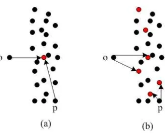
Figure 2.2: Local and global perspectives of outlier-ness of p1 and p2
in detecting both global and local outliers. In the local perspective, human examine the point’s immediate neighborhood and consider it as an outlier if its neighborhood density is low. The global observation considers the dense regions where the data points are densely populated in the data space. Specifically, the neighboring density of the point serves as a good indicator of its outlying degree from the local perspective. In the left sub-figure of Figure 2.2, two square boxes of equal size are used to delimit the neighborhood of points p1 and p2. Because the neighboring density of p1 is less than that of p2, so the outlying degree of p1 is larger than p2. On the other hand,
the distance between the point and the dense regions reflects the similarity between this point and the dense regions. Intuitively, the larger such distance is, the more remarkably p is deviated from the main population of the data points and therefore the higher outlying degree it has, otherwise it is not. In the right sub-figure of 2.2, we can see a dense region and two outlying points, p1 and p2. Because the distance betweenp1 and the dense region is larger than that between p2 and the dense region, so the outlying degree of p1 is larger thanp2.
Based on the above observations, a new measurement of outlying factor of data points, calledOutlying Degree Factor (ODF), is proposed to measure the outlier-ness of points from both the global and local perspectives. The ODF of a pointpis defined as follows:
ODF(p) = k DF(p)
NDF(p)
where k DF(p) denotes the average distance between pand its k nearest dense cells and NDF(p) denotes number of points falling into the cell to whichp belongs.
is used to partition the data space. The main idea of grid-based data space partition is to super-impose a multi-dimensional cube in the data space, with equal-volumed cells. It is characterized by the following advantages. First,NDF(p) can be obtained instantly by simply counting the number of points falling into the cell to which p
belongs, without the involvement of any indexing techniques. Secondly, the dense regions can be efficiently identified, thus the computation of k DF(p) can be very fast. Finally, based on the density of grid cells, we will be able to select the top n
outliers only from a specified number of points viewed as outlier candidates, rather than the whole dataset, and the final top n outliers are selected from these outlier candidates based on the ranking of their ODF values.
The number of outlier candidates is typically 9 or 10 times as large as the number of final outliers to be found (i.e., top n) in order to provide a sufficiently large pool for outlier selection. Let us suppose that the size of outlier candidates ism∗n, where the m is a positive number provided by users. To generate m∗n outlier candidates, all the cells containing points are sorted in ascending order based on their densities, and then the points in the first t cells in the sorting list that satisfy the following inequality are selected as the m∗n outlier candidates:
t−1 X
i=1
Den(Ci)≤m∗n≤ t
X
i=1
Den(Ci)
The kNN-distance methods, which define the top n objects having the highest values of the corresponding outlier-ness metrics as outliers, are advantageous over the local neighborhood methods in that they order the data points based on their relative ranking, rather than on the distance cutoff. Since the value ofn, the top outlier users are interested in, can be very small and is relatively independent of the underlying data set, it will be easier for the users to specify compared to the distance threshold
λ.
C. Advantages and Disadvantages of Distance-based Methods
assumed distribution to fit the data. The distance-based definitions of outliers are fairly straightforward and easy to understand and implement.
Their major drawback is that most of them are not effective in high-dimensional space due to the curse of dimensionality, though one is able to mechanically extend the distance metric, such as Euclidean distance, for dimensional data. The high-dimensional data in real applications are very noisy, and the abnormal deviations may be embedded in some lower-dimensional subspaces that cannot be observed in the full data space. Their definitions of a local neighborhood, irrespective of the circular neighborhood or theknearest neighbors, do not make much sense in high-dimensional space. Since each point tends to be equi-distant with each other as number of dimen-sions goes up, the degree of outlier-ness of each points are approximately identical and significant phenomenon of deviation or abnormality cannot be observed. Thus, none of the data points can be viewed outliers if the concepts of proximity are used to define outliers. In addition, neighborhood andkNN search in high-dimensional space is a non-trivial and expensive task. Straightforward algorithms, such as those based on nested loops, typically requireO(N2) distance computations. This quadratic
scal-ing means that it will be very difficult to mine outliers as we tackle increasscal-ingly larger data sets. This is a major problem for many real databases where there are often millions of records. Thus, these approaches lack a good scalability for large data set. Finally, the existing distance-based methods are not able to deal with data streams due to the difficulty in maintaining a data distribution in the local neighborhood or finding the kNN for the data in the stream.
2.2.3 Density-based Methods
Figure 2.3: A sample dataset showing the advantage of LOF over DB(k, λ)-Outlier
of outliers but require more expensive computation at the same time. What will be discussed in this subsection are the major density-based methods called LOF method, COF method, INFLO method and MDEF method.
A. LOF Method
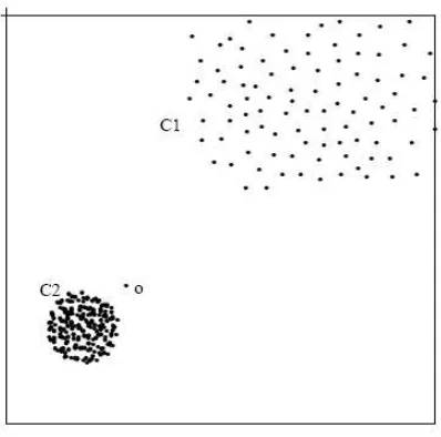
The first major density-based formulation scheme of outlier has been proposed in [26], which is more robust than the distance-based outlier detection methods. An example is given in [26] (refer to figure 2.3), showing the advantage of a density-based method over the distance-based methods such as DB(k, λ)-Outlier. The dataset contains an outlier o, and C1 and C2 are two clusters with very different densities. The DB(k, λ)-Outlier method cannot distinguish o from the rest of the data set no matter what values the parameters k and λ take. This is because the density of o’s neighborhood is very much closer to the that of the points in cluster C1. However, the density-based method, proposed in [26], can handle it successfully.
This density-based formulation quantifies the outlying degree of points usingLocal Outlier Factor (LOF). Given parameter MinP ts, LOF of a point p is defined as
LOFM inP ts(p) =
P
o∈M inP ts(p)
lrdM inP ts(o)
lrdM inP ts(p)
|NM inP ts(p)|
ofpandlrdM inP ts(p) denotes thelocal reachability density of pointpthat is defined as the inverse of the average reachability distance based on the MinP tsnearest neigh-bors of p,i.e.,
lrdM inP ts(p) = 1/ P
o∈M inP ts(p)reach distM inP ts(p, o)
|NM inP ts(p)|
!
Further, the reachability distance of point p is defined as
reach distM inP ts(p, o) =max(MinP ts distance(o), dist(p, o))
Intuitively speaking, LOF of an object reflects the density contrast between its density and those of its neighborhood. The neighborhood is defined by the distance to the MinP tsth nearest neighbor. The local outlier factor is a mean value of the ratio of the density distribution estimate in the neighborhood of the object analyzed to the distribution densities of its neighbors [26]. The lower the density of pand/or the higher the densities ofp’s neighbors, the larger the value ofLOF(p), which indicates that p has a higher degree of being an outlier. A similar outlier-ness metric to LOF, called OPTICS-OF, was proposed in [25].
Unfortunately, the LOF method requires the computation of LOF for all objects in the data set which is rather expensive because it requires a large number of kNN search. The high cost of computing LOF for each data pointpis caused by two factors. First, we have to find theMinP tsth nearest neighbor ofpin order to specify its neigh-borhood. This resembles to computing Dk in detecting Dk
n-Outliers. Secondly, after the MinP tsth-neighborhood of p has been determined, we have to further find the
MinP tsth-neighborhood for each data points falling into theMinP tsth-neighborhood of p. This amounts toMinP tsth times in terms of computation efforts as computing
Dk when we are detecting Dk
n-Outliers.
It is desired to constrain a search to only the top n outliers instead of computing the LOF of every object in the database. The efficiency of this algorithm is boosted by an efficient micro-cluster-based local outlier mining algorithm proposed in [66].
to the choice of MinP ts, the parameter used to specify the local neighborhood.
B. COF Method
As LOF method suffers the drawback that it may miss those potential outliers whose local neighborhood density is very close to that of its neighbors. To address this problem, Tang et al. proposed a new Connectivity-based Outlier Factor (COF) scheme that improves the effectiveness of LOF scheme when a pattern itself has similar neighborhood density as an outlier [111]. In order to model the connectivity of a data point with respect to a group of its neighbors, a set-based nearest path (SBN-path) and further a set-based nearest trail (SBN-trail), originated from this data point, are defined. This SNB trail stating from a point is considered to be the pattern presented by the neighbors of this point. Based on SNB trail, the cost of this trail, a weighted sum of the cost of all its constituting edges, is computed. The final outlier-ness metric, COF, of a point p with respect to its k-neighborhood is defined as
COFk(p) = |Nk(p)| ∗ac distNk(p)(p)
P
o∈Nk(p)ac distNk(o)(o)
where ac distNk(p)(p) is the average chaining distance from point p to the rest of its
k nearest neighbors, which is the weighted sum of the cost of the SBN-trail starting fromp.
It has been shown in [111] that COF method is able to detect outlier more ef-fectively than LOF method for some cases. However, COF method requires more expensive computations than LOF and the time complexity is in the order ofO(N2)
for high-dimensional datasets.
C. INFLO Method
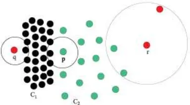
Figure 2.4: An example where LOF does not work
obviously displays less outlier-ness. However, if LOF is used in this case, p could be mistakenly regarded to having stronger outlier-ness than q and r.
Authors in [67] pointed out that this problem of LOF is due to the inaccurate specification of the space where LOF is applied. To solve this problem of LOF, an improved method, called INFLO, is proposed [67]. The idea of INFLO is that both the nearest neighbors (NNs) and reverse nearest neighbors (RNNs) of a data point are taken into account in order to get a better estimation of the neighborhood’s density distribution. The RNNs of an objectpare those data points that havepas one of their
knearest neighbors. By considering the symmetric neighborhood relationship of both NN and RNN, the space of an object influenced by other objects is well determined. This space is called the k-influence space of a data point. The outlier-ness of a data point, called INFLuenced Outlierness (INFLO), is quantified. INFLO of a data point
p is defined as
INF LOk(p) = denavg(ISk(p))
den(p)
Figure 2.5: Definition of MDEF
D. MDEF Method
In [95], a new density-based outlier definition, called Multi-granularity Devia-tion Factor (MEDF), is proposed. Intuitively, the MDEF at radius r for a point
pi is the relative deviation of its local neighborhood density from the average local neighborhood density in its r-neighborhood. Let n(pi, αr) be the number of objects in the αr-neighborhood of pi and ˆn(pi, r, α) be the average, over all objects p in the r-neighborhood of pi, of n(p, αr). In the example given by Figure 2.5, we have
n(pi, αr) = 1, and ˆn(pi, r, α) = (1 + 6 + 5 + 1)/4 = 3.25. MDEF of pi, givenr and α, is defined as
MDEF(pi, r, α) = 1−
n(pi, αr) ˆ
n(pi, r, α) where α= 1
2. A number of different values are set for the sampling radius r and the
minimum and the maximum values for r are denoted by rmin and rmax. A point is flagged as an outliers if for any r∈[rmin, rmax], its MDEF is sufficient large.
E. Advantages and Disadvantages of Density-based Methods