Extreme Events: a physical reconstruction and risk assessment

(1)

Extreme Events

A Physical Reconstruction and Risk Assessment

The assessment of risks posed by natural hazards such as ﬂoods, droughts, earthquakes, tsunamis or tropical cyclones is often based on short-term historical records that may not reﬂect the full range or magnitude of events possible. As human populations grow, especially in hazard-prone areas,

methods for accurately assessing natural hazard risk are becoming increasingly important.

InExtreme EventsJonathan Nott describes the many methods used to reconstruct such hazards from natural long-term records. He demonstrates how long-term (multi-century to millennial) records of natural hazards are essential in gaining a realistic understanding of the variability of natural hazards likely to occur at a particular location. He also demonstrates how short-term historical records often do not record this variability and can therefore misrepresent the likely risks associated with natural hazards.

This book will provide a useful resource for students taking courses

covering natural hazards and risk assessment. It will also be valuable for urban planners, policy makers and non-specialists as a guide to understanding and reconstructing long-term records of natural hazards.

J o n a t h a n N o t t _{is Professor of Geomorphology at James Cook University in} Queensland, Australia. His broad research interests are in Quaternary climate change and the reconstruction of prehistoric natural hazards. Other research interests include long-term landform evolution, plunge pool deposits

(2)

Extreme Events

A Physical Reconstruction

and Risk Assessment

(3)

c a m b r i d g e u n i v e r s i t y p r e s s

Cambridge, New York, Melbourne, Madrid, Cape Town, Singapore, S˜ao Paulo

Cambridge University Press

The Edinburgh Building, Cambridge CB2 2RU, UK

Published in the United States of America by Cambridge University Press, New York

www.cambridge.org

Information on this title: www.cambridge.org/9780521824125

C

J. Nott 2006

This publication is in copyright. Subject to statutory exception and to the provisions of relevant collective licensing agreements, no reproduction of any part may take place without

the written permission of Cambridge University Press.

First published 2006

Printed in the United Kingdom at the University Press, Cambridge

A catalogue record for this publication is available from the British Library

ISBN-13 978-0-521-82412-5 hardback ISBN-10 0-521-82412-5 hardback

(4)

(5)

Acknowledgments

I would like to thank Drs Scott Smithers and James Goff for their constructive comments on this manuscript. Their assistance was invaluable. The views expressed in this book are entirely mine.

I would also like to thank the following for permission to reproduce in part and/or full the following:

Elsevier Science for Figures 2.1, 2.8, 2.9, 5.9, 6.4, 6.5, 7.4, 7.5, 7.6, 7.7, 7.8, 8.2, 8.4. Nature Publishing Group for Figures 2.4, 2.5, 2.6, 2.10, 4.3, 4.11.

Geological Society of America for Figures 2.2, 7.2, 7.3. American Geophysical Union for Figures 5.7, 7.9, 7.10, 8.3. Coastal Research Foundation or Figure 2.4.

National Atmospheric and Oceanic Administration for Figure 2.11, 2.12. Professor D.A. Kring for Figures 9.1, 9.2, 9.3, 9.4, 9.5.

(10)

1 Introduction

The problem with natural hazard risk assessments

(11)

2 Extreme Events

to interpret this natural variability. Nature, however, effectively records its own extreme events, and often its not so extreme ones, providing us with a docu-mented history in the form of natural records that can display the full range of variability of most hazards that confront society. Long-term records, there-fore, are the only real source for uncovering the true nature of the behaviour of natural hazards over time.

Scientists who study the Quaternary -- the most recent period of geologi-cal time (or approximately the last 2 million years) know that natural events including hazards often occur in clusters or at regular to quasi-periodicities. Over longer time intervals, the Quaternary record shows us that the periodic-ity of events, including climatic changes, is governed by many factors, some of which are external to the Earth. For example, climatic changes of various scales occur at intervals from 100 000 years to 11 years based upon regular variations in the orbit of the Earth around the Sun, along with the tilt of the Earth’s axis and precession of the equinoxes, to sunspot activity. There are many other regular cycles of climate change that occur in between the 100 000 and 11 year cycles that have been uncovered from a variety of natural records. The clear message from Quaternary records is that many of the climatic changes that occur on Earth do not occur randomly and in this sense are not independent of time. The same could be expected of many extreme natural events.

While it is true that natural records do not document the event as accurately as the instrumented record, they are nonetheless of sufﬁcient precision to show us the magnitude of the most extreme events and how often these events are likely to occur. Even more importantly, natural records provide us with a very effective means by which to test the assumptions of the stationarity of the mean and variance, and randomness of occurrence of a natural hazard. In the absence of these tests we cannot hope to realistically assess community vulnerability and exposure, and therefore risk. Social scientists, involved in that part of the risk evaluation process devoted to community and social parameters, also need to be aware of the assumptions made by scientists and engineers in determining the physical nature of the hazard. This is frequently not the case and planners are left with false impressions of which areas are safe for urban, industrial and tourism developments.

(12)

Introduction 3

risk assessments. Through familiarity, though, comes awareness of the insights that the prehistoric record can provide into gaining a more realistic impression of the behaviour of natural hazards.

The risk assessment process

Risk from natural hazards is a function of the nature of the natural hazard (i.e. probability of its occurrence), community vulnerability and the ele-ments at risk. Risk can have a variety of meanings and is sometimes used in the sense of the probability or chance that an event will happen within a specific period of time. Alternatively, risk can refer to the outcomes of an event occur-ring. In this latter sense, risk refers to the expected number of lives lost, persons injured, damage to property and disruption of economic activity due to a partic-ular natural phenomenon. Risk is really the product of the specific risk and the elements at risk. The specific risk here means the expected degree of loss due to a particular natural phenomenon and is a function of both the natural hazard and vulnerability (Fournier d’Albe, 1986). The elements at risk, otherwise known as the level of exposure, refers to the population, buildings, economic activities, public services, utilities and infrastructure that may be directly impacted by the hazard.

Community vulnerability is determined by the social and demographic attributes that inﬂuence a person’s perception of the risk to the hazard. It often concerns peoples’ attitudes, preparedness and willingness to respond to warnings of an impending hazard. Anderson-Berry (2003) notes that community vulnerability is not a static state but a dynamic process. It is generated by the complex relationships and inter-relationships arising from the unique actions and interactions of the social and community attributes and characteristics of a particular population.

These attributes and characteristics include:

r _{societal structures, infrastructure and institutions including the}

integrity of physical structures;

r _{community processes and structures such as community organisation,}

mobility of the household population, and community cohesiveness and the social support this affords; and

r _{demographic and other characteristics of individuals within the}

com-munity such as age, ethnicity, education and wealth (Keys, 1991; Fothergill, 1996; Buckle, 1999; Fothergillet al., 1999; Cannon, 2000).

(13)

4 Extreme Events

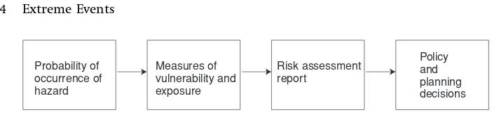
Probability of occurrence of hazard

Measures of vulnerability and exposure

Risk assessment report

[image:13.468.56.412.119.203.2]

Policy and planning decisions

Figure 1.1. Generalised sequence of process occurring in a risk assessment. In

reality there are many feedback loops between the steps outlined here.

(2003) notes that people individually and collectively decide what precautionary measures will be undertaken and how warnings will be complied with so as to ensure that the loss resulting from a hazard event is limited to an acceptable level. If the perceived risk is a true reﬂection of the actual risk associated with a particular hazard, then mitigation strategies, warning compliance and response preparedness are likely to be appropriate and vulnerability can be minimised. If risk perception is biased, the reverse is true and vulnerability may be increased. The perception of risk, therefore, can often be the precursor to determining the level of exposure to that risk, although it is true that perceptions can and do change over time. So increasing awareness with time, due to education about or experience with the hazard may result in the realisation that more elements are exposed than previously thought. The level of exposure, therefore, is a function of past and present perceptions of risk.

The total risk is often expressed as:

risk (total)=hazard×elements at risk×vulnerability

(14)

Introduction 5

Each of these stages is critical and no less valuable than the others in terms of reducing risk from natural hazards. However, any variation to the outcome of the ﬁrst stage (i.e. the hazard probability) inﬂuences each of the other stages; hence, each of the latter are dependent on the former. For example, hundreds to thousands more homes may be deemed to be exposed to tsunami inundation depending upon whether the assessed probability of occurrence of tsunami run-up height is 1 or 2 m above a certain datum for a given time interval along a densely populated low-lying coast. Likewise, government policy decisions may set aside a considerably larger area of coastal land deemed to be unsuitable for permanent development depending upon the height of the tsunami run-up determined. Obtaining the most accurate and realistic estimate of the magnitude of a hazard at a given probability level, therefore, is usually in the best interests of all concerned in the risk assessment process, and likely even more so for those potentially subject to impact by the hazard. The perception of the most realistic estimate, however, can vary and is the essence of the earlier stated problem in the risk assessment process. There can be a difference between the mathematical and/or statistical certainty of a certain magnitude hazard occurring in a given time period and the so-called realistic estimate of the size of that hazard.

Mathematical and statistical certainties versus realistic estimates

(15)

6 Extreme Events

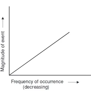
Frequency of occurrence (decreasing)

Magnitude of e

v

[image:15.468.109.261.137.289.2]

ent

Figure 1.2. Typical relationship between event magnitude and frequency. Note that

larger magnitude events occur less frequently than smaller magnitude events.

any one year always remains the same. In fact, its probability of occurrence is regarded as remaining the same for any period of time. This remains the case if the event occurs independently of prior events and therefore, like the toss of a coin, occurs randomly within any given period of time. If external factors influence the occurrence of that event then it will not be occurring independently of a specified period of time. To once again use the coin tossing analogy, if something influences the outcome of the tosses of a coin for some specific period of time then we can no longer say that the outcome is a random occurrence. We know that this is unlikely to be the case when tossing a coin, but it is a very real possibility with respect to the occurrence of natural hazards over time.

There are statistical measures, such as Bayesian analyses, which do assume that prior events inﬂuence the occurrence of subsequent events and these are sometimes used in risk assessments of some natural hazards such as earth-quakes. Bayesian analysis is usually only used for hazards that have known build-up and relaxation times, as occurs for example when crustal stresses along a fault or tectonic plate boundary build to the point of release causing an earth-quake. Following the earthquake, it takes some time for those stresses to once again build to a level to induce the next earthquake. So the time between earth-quakes is not random and the probability of an earthquake occurring at that speciﬁc location is reduced for a period and hence varies over time. This can be called a conditional probability. Other hazards, such as many atmospheric hazards, however, where such processes are thought not to operate, are gener-ally regarded as occurring randomly with respect to previous events and in this sense randomly with respect to time.

(16)

[image:16.468.56.403.163.283.2]

Introduction 7

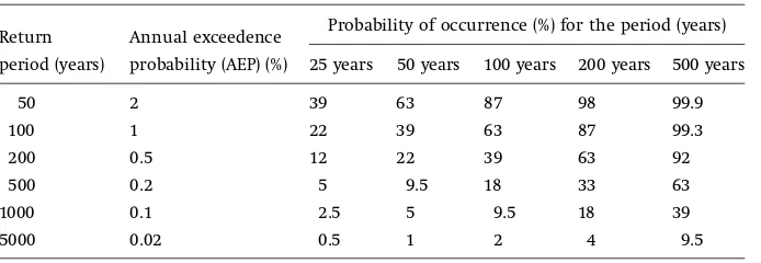
Table 1.1 Percentage probabilities of occurrence for given time intervals

Probability of occurrence (%) for the period (years) Return

period (years)

Annual exceedence

probability (AEP) (%) 25 years 50 years 100 years 200 years 500 years 50 2 39 63 87 98 99.9 100 1 22 39 63 87 99.3 200 0.5 12 22 39 63 92 500 0.2 5 9.5 18 33 63 1000 0.1 2.5 5 9.5 18 39 5000 0.02 0.5 1 2 4 9.5

more likely, therefore, that a place will experience a high-magnitude event with increasing time. So location X, for example, is unlikely to experience a high-magnitude event over 100 years but is reasonably likely to experience this event over a 1000 year period. But, as stated earlier, the likelihood of that high-magnitude event occurring in any 100 year period remains the same, even if it has been 900 years since the last high-magnitude event. The probability of that event occurring between year 900 and year 1000 is exactly the same as the probability of occurrence between year 100 and year 200. Probabilities, there-fore, are determined according to the time interval to which they pertain. The probability of the 1 in 100 year event (1% annual exceedence probability, AEP) occurring is 1/100 in any given year. In other words, this event has a 1% chance of occurring in any given year. Likewise, it has a 39% chance of occurring in a 50 year period, 63% chance of occurring in a 100 year period and 99.3% chance of occurring in a 500 year period. Table 1.1 sets out the probabilities of events occurring over various time intervals. The determination of these probabilities is calculated according to the binomial distribution. The equation for the binomial distribution is

P(r)=n_Crpr_qn−r _(1.1)

where n_C

r (the binomial coefﬁcient) = n! /r!(n− r)! and where P(r) is the

prob-ability of occurrence, nis the number of events in the record, r = 0 andq = 1−p.

The binomial distribution is based upon the randomness of occurrence of events over time. The same distribution is used to explain the chance of obtain-ing a head or tail in the toss of a coin which is most certainly a random event. By applying the same statistical probability distribution to the occurrence of natural hazards we make the assumption that these events occur randomly like the chance of obtaining a head or tail in the toss of a coin.

(17)

8 Extreme Events

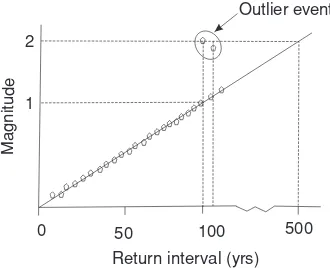
0 50 100

Magnitude

Return interval (yrs) 500 Outlier events

[image:17.468.109.274.148.282.2]

1 2

Figure 1.3. Magnitude--frequency curve and outlier points.

can be seen to fall roughly on a straight line; however, two events do not. These two events are referred to as ‘outliers’ and they are of higher magnitude than any other events to have occurred over the past 100 years. The probability dis-tribution suggests that despite the fact that these outlier events have occurred within the last 110 years they do not belong to the normal range of events that could be expected to occur within this time frame. By extending the line repre-senting the magnitude--frequency relationship for this particular hazard, these events appear more likely to correspond to the approximately 1 in 500 year event (0.2% AEP). Such a conclusion is ﬁrmly based upon the assumption that the slope of the line representing the magnitude--frequency relationship is applicable to any 100 year period. Therefore, this line, which only covers events from the last 100 years, is typical of any 100 year period. When we make this assumption we also deem it safe to extrapolate this line to determine an accurate estimate of the size of less frequent events. Whether this is a realistic interpretation of the nature of the natural hazard, however, is rarely ever tested during the risk assessment process. Nor is the possibility that non-stationarity may be evident when longer time series or records of events are examined. In the above situa-tion stasitua-tionarity has been assumed. Unfortunately though, nature rarely displays stationarity over the long term.

Stationarity in time series

(18)

Introduction 9

Decreasing frequency of event occurrence

Increasing magnitude of e

v

ent

Tim e 1

Time 2

T1

T2

[image:18.468.94.312.146.355.2]

X

Figure 1.4. Non-homogeneity of magnitude--frequency relationship over time.

the line steepens, events of greater magnitude will occur more frequently. The converse is true when the slope of the line decreases. These changing relation-ships are shown in Figure 1.4. Two lines are presented here. Each line represents a different relationship between the frequency of occurrence of an event and its associated magnitude. An event with frequencyX will have a magnitude of T1 during a period named here as Time 1, and magnitudeT2 during the period

Time 2. These periods may be years, decades, centuries or millennia in length. This is non-stationarity (see Fig. 1.5).

(19)

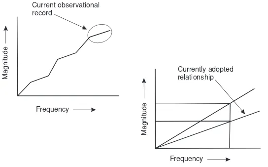
10 Extreme Events

Frequency

Magnitude

Frequency Current observational

record

[image:19.468.107.379.147.316.2]

Currently adopted relationship

Figure 1.5. Non-stationarity in the time series.

community vulnerability and levels of exposure. If we believe that the high-magnitude event is an outlier then we will believe that the chances of an event of similar size occurring during the next planning cycle, or the near future, are low (i.e. as set out in Table 1.1). For example, if we perceive the outlier event to be a 1 in 500 year event (0.2% AEP) then we will draw the conclusion that its chances of occurring in the next 50 years are less than 10%. However, if we ﬁnd from a longer-term record that this magnitude event is really more likely to be a 1 in 100 year event (and indeed it did occur only a little over 100 years ago in reality) then its chance of occurring in the next 50 years is about 39%. Alternatively, it could be an event that signals the onset of a change in hazard behaviour. Either way, when we assume it was a 1 in 500 year event, and ignore the possibility that it is part of a normal series of events for a regime that was not recognised due to the brevity of the observational record, then we will have placed potentially large numbers of people and property at higher than pre-dicted levels of risk. Each change of phase in hazard behaviour, i.e. change of slope in the magnitude--frequency curve, can be referred to as a hazard regime (Nott, 2003). These regimes can be likened to alternating periods of variable sta-tionarity. Recognising the possibility that these regimes may exist for a hazard at any location can only help us to gain a more realistic view of the nature of the hazard.

Reality versus reasonableness