Stability Analysis of Nonlinear Power Electronic
Systems Utilizing Periodicity and Introducing
Auxiliary State Vector
Octavian Dranga, Balázs Buti, István Nagy
, Fellow, IEEE
, and Hirohito Funato
, Member, IEEE
Abstract—Variable-structure piecewise-linear nonlinear dy-namic feedback systems emerge frequently in power electronics. This paper is concerned with the stability analysis of these sys-tems. Although it applies the usual well-known and widely used approach, namely, the eigenvalues of the Jacobian matrix of the Poincaré map function belonging to a fixed point of the system to ascertain the stability, this paper offers two contributions for simplification as well that utilize the periodicity of the structure or configuration sequence and apply an alternative simpler and faster method for the determination of the Jacobian matrix. The new method works with differences of state variables rather than derivatives of the Poincaré map function (PMF) and offers geometric interpretations for each step. The determination of the derivates of PMF is not needed. A key element is the introduction of the so-called auxiliary state vector for preserving the switching instant belonging to the periodic steady-state unchanged even after the small deviations of the system orbit around the fixed point. In addition, the application of the method is illustrated on a resonant dc–dc buck converter.
Index Terms—DC–DC power conversion, nonlinear systems, sta-bility, variable-structure systems.
I. INTRODUCTION
L
ARGE numbers of converters in power electronics be-long to the variable-structure, piecewise-linear nonlinear dynamic feedback systems. They change their structure and their configuration after each switching, and the sequence of structures succeeds each other periodically in the periodic steady state. Each structure of the converters can be modeled with good approximation by linear circuitry, and therefore they are piecewise linear. The overall systems are nonlinear due to the dependence of switching instants on state variablesManuscript received March 19, 2003, revised August 2, 2004. This work was supported by the Hungarian Research Fund under Grant OTKA TO34654, Grant OTKA TO34630, and Grant OTKA TO46240, and by the Control Research Group of the Hungarian Academy of Science. This paper was recommended by Associate Editor M. K. Kazimierczuk.
O. Dranga is with the Department of Electronic and Information Engi-neering, The Hong Kong Polytechnic University, Kowloon, Hong Kong (e-mail: [email protected]).
B. Buti is with the Department of Automation and Applied Informatics, Bu-dapest University of Technology and Economics, H-1111 BuBu-dapest, Hungary (e-mail: [email protected]).
I. Nagy is with the Department of Automation and Applied Informatics, Bu-dapest University of Technology and Economics, H-1111 BuBu-dapest, Hungary, and also with the Computer and Automation Institute, Hungarian Academy of Sciences, H-1111 Budapest, Hungary (e-mail: [email protected]).
H. Funato is with the Department of Electrical and Electronic Engineering, Utsunomiya University, Utsunomiya 321-8585, Japan (e-mail: funato@ cc.utsunomiya-u.ac.jp).
Digital Object Identifier 10.1109/TCSI.2004.840102
stemming from the feedback control loop and due to saturation or other nonlinearities.
The paper is concerned with the stability of such systems. Be-sides the periodicity of the configuration sequence, the switch-ings have to be controlled by pulse width modulation (PWM) in the system. It must be emphasized that the stability study used in the paper is based on the well-known and widely applied ap-proach in which the eigenvalues of the Jacobian matrix of the Poincaré map function are determined at a fixed point of the system [1]–[12]. From a physical viewpoint, it is equivalent to study the behavior of the trajectory of the system in state space when it is forced to leave its periodic steady-state trajectory to a new orbit by a small deviation from the original trajectory.
This paper offers new contributions, to the best of the authors’ knowledge, to the usual stability analysis in two points. The first point is utilizing the periodicity of the structure sequence and introducing subperiods. State equations have to be derived only for one subperiod, which reduces the number of state equations needed for the stability analysis. We do not consider it as major contribution but it can be very useful. This method has already been used once [13], but it has not been introduced in a generic way. Second, and most important, we determine the Jacobian matrix by using the small differences of state vectors compared to their steady-state values at the start and end of subperiods and at the switching instant. There is no need to determine the derivates of the Poincaré map function at the fixed point. The Jacobian matrix is obtained directly from the relations among the small differences of state vectors. In addition, all steps are interpreted graphically. Consequently, this method offers an al-ternative way to derive the Jacobian matrix or, which is more significant, a simpler and faster way to determine it. The key element of this method is the introduction of the auxiliary state vector for preserving constant switching instants for the switch-ings depending on state variables even after the small excursion of the state variables from the steady state, although they vary in small extent.
The method is described in a generic way in Sections II–V. The application of the method is illustrated with a dual channel dc–dc resonant converter in Sections VI and VII and the Appendix).
II. POWER ELECTRONIC CIRCUITS AS
VARIABLE-STRUCTURESYSTEMS
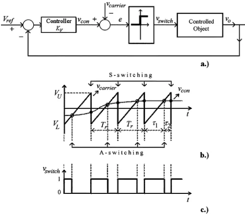
Fig. 1(a) presents the simplified block diagram of the type of systems discussed. The controlled object is the
Fig. 1. Time sequence of structure changes in the periodic steady state.
[image:2.594.40.287.67.166.2]ture power part with controlled switches, incorporating period-ically changing subcircuits, which are cyclperiod-ically turned on and off. The output voltage is controlled by PWM. The carrier signal can be, e.g., a ramp function (saw-tooth wave-form) [see Fig. 1(b)]. The output signal of the controller is compared to the carrier signal . The state of the controlled switches depends on the sign of . Having only one switch in the controlled object in the simplest case, the pe-riod of the ramp signal and the period of the state variables are equal to each other as in a hard-switched buck, boost and buck, and boost dc–dc converters [Fig. 1(b)]. When two con-trolled switches are in the concon-trolled object and they are turned on and off alternately, as we will see in our example, . Switching occurs in the controlled object at each transition in from 0 to 1 orvice-versa. Two kinds of switching take place: asynchronous A-switching and synchronous S-switching [Fig. 1(b)].
In order to make as clear and simple as possible the descrip-tion of the alternative method of deriving the Jacobian matrix within the frame of stability study, which is the main target of the paper, the simple proportional controller
(1) will be assumed.
The controlled object is a variable-structure piecewise-linear system. After each switch, another linear circuit emerges and the sequence of linear circuits is repeated in the next period [13].
Fig. 2 shows the time sequence of structure changes within one period as a simple example. The dual-channel resonant dc–dc converter has, in fact, this sequence of structure changes, as will be shown later on. Here, one period has two subperiods , where is the number of subperiods in one pe-riod and each subpepe-riod consists of two linear circuits called structures . Suffixes , and
are used for counting the number of periods and subperiods starting from the beginning of the transient process, respectively.
Building up a linear circuit model on the basis of the actual configuration of the power electronics converter corresponding to the actual state of the switches, the model is the same for structure 1 in subperiod I and for structure 1* in subperiod II. The same statement holds for structures 2 and 2*. Therefore, the sequence of models repeats itself in each subperiod. At the same time, the actual energy storage components, resistances, switches, and the associated state variables belonging to the
Fig. 2. (a) Block diagram of the variable-structure piecewise-linear feedback system controlled by PWM. (b) Carrier signal is a saw-tooth wave. (c) Switching signalv .
same successive structures (e.g., structures 1 and 1*) might be partially or entirely different.
Due to the identical structures (1 and 1* as well as 2 and 2*) in the two subperiods, the state equations in the two intervals (and in the two intervals) have the same mathematical forms. The state variables can be different in the same places of the equations, but the values of the parameters are the same due to symmetry. The identity of the form of state equations makes it possible to calculate the dynamic processes in subperiod II and, in general, in subperiod by using only the state equations of subperiod I. The state vector at the end of subperiod I has to be transformed back in an appropriate way to the starting state vector of subperiod I (Section III). The state variables of subperiod I are used for the calculation of state variables of subperiod II. Their identification with the actual state variables of subperiod II that they represent can easily be done. Applying only the state equations of subperiod I together with the back transformation, the whole period can be treated.
The method described in the paper can be extended for sys-tems with a more sophisticated structure sequence if otherwise the systems meet the other restrictions described.
III. MATHEMATICALBACKGROUND
Everything in this section is well known except the concept of back transformation. The aim of this section is mainly the introduction of notations used later on.
The variable-structure system shown in Fig. 1(a) is nonau-tonomous due to signal [1]–[3]. The controlled object within structures 1 and 2 is linear, and it can be described by the coupled first-order linear differential equation system or state equation
in the interval (Fig. 2) where is the velocity vector, is the state vector, and is the excitation vector. Ma-trices and depend on the configuration and parameters of the respective structure in the controlled object. At the switching instant, the velocity vector is suddenly changed, e.g., at (Fig. 2) as follows:
(3) where suffixes and stand for start and end, respectively. acts upon the system as a “force,” and the direction of the system trajectory is abruptly varied in the state space.
The solution of (2) is well known, and its expression is (4) where suffix has been dropped, and is the time elapsed from the switching instant. The weighting matrix
(5) and the particular solution from (2) is
Having two structures within a subperiod (Fig. 2), (4) has to be applied twice, always with the respective values pertaining to the actual structure.
In the steady state, the periodicity or transfer matrix con-nects the values of the state vector at the start and the end of the subperiod I
(6) or
(7) where the elements in matrix are , or 0 (cf. the example in Section VI and in the Appendix) and
(Fig. 2). Suffixes 1 and 2 stand for structures 1 and 2, re-spectively. Knowing the operation of the respective power elec-tronics configuration, the determination of is a simple task, as will be seen later on. Equation (7) can be interpreted as follows. After calculating , the operation is a back trans-formation of to the start of subperiod I in order to apply as the initial value in the same state equations (that were used in subperiod I) for the calculations of the state variables in subperiod II.
The interval (and ) can be determined from the rule of PWM switching (1) and Fig. 1(b)
(8) Although the equations of the controlled object (2) and (7) are linear, the last relation (8) is nonlinear due to the dependence of on the state variable [and because can be higher than or lower than ; see Fig. 1(b)], resulting in no switching in one or more consecutive subperiods). In general, the cal-culation of from the nonlinear equation leads to an iteration procedure.
IV. SMALLCHANGESAROUND THEPERIODIC STATE ANDAUXILIARYSTATEVECTOR
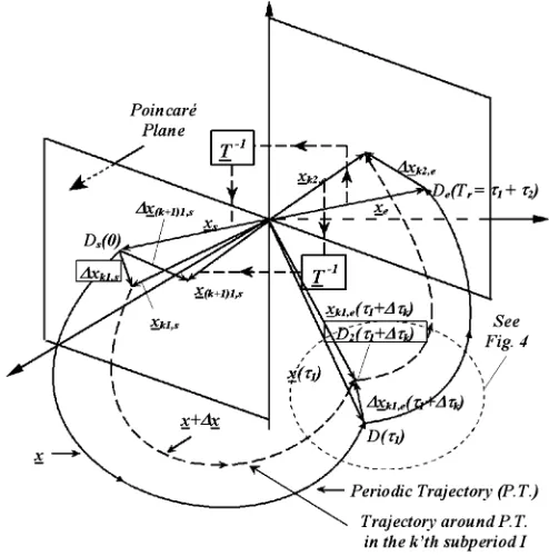
[image:3.594.303.550.66.316.2]The system trajectory keeps circulating along the same closed loop in state space in the periodic state. As an example, Fig. 3
Fig. 3. Back transformation of x to the start of the next subperiod I. Trajectory in the steady state (heavy solid line). Trajectory after small deviation from the steady state (dashed line).
shows the trajectory of state vector and its start and end positions in subperiod I in the steady state in three-dimen-sional (3-D) state space (heavy solid line). In the periodic steady state, the trajectory pierces through the Poincaré plane at point where the state vector is , which is the fixed point. After subperiod I, the state vector is (point ). Transforming back to the start of subperiod I by matrix , the original state vector is reobtained: [(7)]. The system trajec-tory starts from the fixed point again.
Due to a small deviation of the trajectory from point , the small change in the state vector at the start of the th subperiod I is and the state vector is in Fig. 3. At the end of the th subperiod I, the state vector is . Suffixes 1 and 2 refer to structures 1 and 2, respectively (Fig. 2). Transforming back to the start of the th subperiod, we obtain
(9) As a result of the small deviation around the periodic state, remains unchanged but, in general, is changed in the th subperiod by due to its dependence on the changing state variable [Fig. 1(b) and (8)]. varies from subperiod to subperiod. (It is assumed that holds.) The stability calculation or, more precisely, the calculation of the Jacobian matrix is greatly simplified by introducing anauxiliary
state vector at the structure change from 1 to 2 at
(Fig. 2) and itschange in place of the actual state vector change (Fig. 4). This permits us to take into account the effect of the change but at the same time keep and, consequently, unchanged. The rewards of this method are as follows.
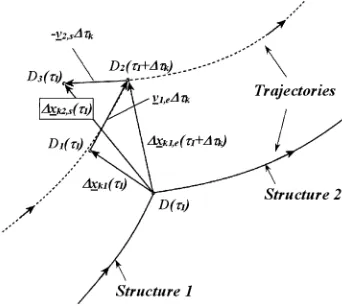
Fig. 4. Auxiliary state vector change1x ( )(see Fig. 3).
2) The Jacobian matrix is directly obtained from the re-lations among the small changes of the state vectors written on the basis of Figs. 3 and 4 and from (8) rewritten for small changes. The equations have graph-ical interpretation.
3) Weighting matrices and can be ap-plied for small changes as well.
has to be calculated by an iteration process only once for the periodic steady state. The description of the iteration process for the calculation of is straightforward and beyond the scope of this paper. we refer the reader to [13].
On the basis of (4), the relation between the small changes of the state vector in structures 1 and 2 are as follows (Fig. 4):
(10) (11) where is the small change in the state vector at , that is, in advance by before the end of the th subperiod I. By knowing structures 1 and 2, we know and ; therefore, the determination of and is straightforward.
All small changes are real values, but the fictitious auxiliary state vector change can be determined from
(12) where matrix can be derived from Fig. 4, as will be shown later.
The starting point is the periodic trajectory or limit cycle of the system. A small section of the trajectory in the neighbor-hood of the switching from structure 1 to structure 2 is shown by the heavy solid line in Fig. 4, which is a blow up around point in Fig. 3. The trajectory reaches the switching hy-persurface at point in the periodic steady state where the velocity vector is abruptly changed [(3)]. After deviating the system from its limit cycle by a tiny change, the dashed line illustrates the corresponding section of the new trajectory around point , where the switching hypersurface is reached by this new trajectory at The “distance” be-tween and is , where is the velocity vector at point still in structure 1. The alteration of the state vector on the hypersurface is . After the switching, the velocity vector at the start of structure 2 is at point
. The determination of and will be discussed soon. Due to the linearity of the structures, the new trajectory can be projected “backward in time” from time to . In other words, the trajectory will start from point rather than point by extending the new trajectory at the start of structure 2 toward “negative time” in the direction of the velocity vector . Point is reached this way at distance from Theauxiliary state vector change
is obtained between points and . This math-ematical abstraction is useful since, by applying in place of , the trajectory will start in structure 2 at the same instant as in the case of the periodic trajectory. Turning to the determination of the relation between the real state vector change and the auxiliary one , the following relationship is obtained from triangles
and :
(13) By introducing theauxiliary state vector
directed to point and theauxiliary state vector change
, the application of as the unchanged interval for structure 1 is still permitted in the relations among the small deviations.
V. DETERMINATION OF THEJACOBIANMATRIX ON THEBASIS OF THEAUXILIARYSTATEVECTOR
The aim is the determination of , the Jacobian matrix of the subperiods belonging to the fixed point . The relation among the consecutive small deviations of the state vector around the fixed point is
(14) where is the initial deviation of state vector at fixed point .
At the start of the th subperiod, we have
(15) where is the Jacobian matrix of the whole switching period
. Therefore
(16) The eigenvalues of Jacobian matrix equals the square of those of Jacobian matrix . The stability of the fixed point can be concluded either from or . When the eigenvalues of are within the unit circle, those of are inside the unit circle as well, andvice-versa.
After determining from (10), the next step is the calculation of the auxiliary state vector change from (12). We have to know matrix at this step. can be derived from (13) if can be expressed by .
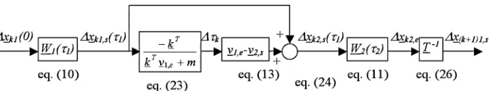
Fig. 5. Calculation sequence of the Jacobian matrixJ .
of constant vector are zero except one (or two, see later1)
belonging to . The transposition of vector is denoted by . The relation for is [Fig. 1(b)]
(17) Equation (8) can be rewritten at as
(18) and at as
(19) Subtracting (19) from (18) yields
(20) From triangle , we have
(21) Substituting (21) into (20) yields
(22) and from here
(23)
Substituting from (23) into (13) results in the following relationship for which we are looking:
(24) where is theauxiliary state vector changeat the start of structure 2 and is the identity or unit matrix. Equation (24) determines matrix introduced in (12). Theauxiliary state
vector change permitting us to calculate with the
constant switching interval can be determined by matrix from state vector change .
Applying (10)–(12) in cascade for the entire th subperiod I yields
(25)
1In the example, in Section VIv = v + v and bothv andv are state variables [(A1)].
Note that (25) is the same in each subperiod. Due to the period-icity, has to be transformed back to the start of subperiod I [see Figs. 2 and 3 and (9)] to yield
(26) Comparing (14) and (26), the Jacobian matrix is
(27)
A. Speed Vectors
To determine the speed vectors and , first we have to know the state vector at the fixed point. Assuming that we know and applying (4), the state vector at
(28) and at the end of subperiod I
(29) where is assumed.
In steady state
(30) From the last equations, we have
(31) By knowing from (28), the velocity vector from (2) yields
(32) (33)
On the basis of (28)–(30), the PMF is
Fig. 6. (a) General configuration of the converters. (b), (c) Basic building blocks.
TABLE I
SETUP OF THECONVERTERS
We did not apply the derivative of in the derivation of the Jacobian matrix .
[image:6.594.313.541.206.370.2]Now that we know all terms in matrix , its eigenvalues and, similarly, the eigenvalues of the Jacobian matrix can be calculated, that is, the stability of the periodic state can be ascertained.
Fig. 5 summarizes the calculation sequence of the Jacobian matrix . It can be concluded that the derivatives of the PMF are not needed for the determination of the Jacobian matrix. Ref-erence [13] discusses the determination of the Jacobian matrix for exactly the same type of power electronics systems using the traditional approach, that is, from the derivatives of the PMF. The comparison shows clearly how much simpler and faster the direct method is than the traditional one (see [13, Secs. VI-B and C] and compare it with Section V of this paper); of course, the results are the same. Compare (24) and (27) to [13, eqs. (37) and (38)].
VI. EXAMPLE: DC–DC CONVERTER
CONFIGURATION ANDOPERATION
As an example, a dual-channel resonant buck configuration is chosen. The converter is a member of a converter family. A com-prehensive study of the family has been published earlier [26]. Here, only a short description of the configurations and the op-eration of the members of the family is given. It was previously studied in [13] and [25] by using the traditional approach for determining the Jacobian matrix.
The general configuration of the family shown in Fig. 6(a) has a positive (suffix ) and a negative (suffix ) channel, two switched capacitors , two basic building blocks and , two filter capacitors and , and the loads and . Suffixes and refer to input and output, respec-tively. The configurations of the basic building blocks can be
Fig. 7. Time functions of input and output (inductor) currents(! = 1=pLC).
Fig. 8. Bifurcation diagram: I—periodic range; II—quasi-periodic and subharmonic range; III—chaotic and subharmonic range.
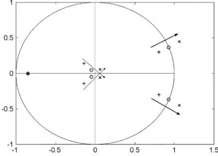
Fig. 9. Loci of eigenvalues(R = 6 )as the controller gainK varies. Arrows indicate increasing gain.
either or with two controlled switches and and inductance [see Fig. 6(b) and (c)]. The controlled switches (IGBTs, MOSFETs, or other switches) conduct current in the direction of the arrow.
Using the general configuration, any one of the buck, buck and boost, or boost converters can be built by connecting the , and terminals of the basic building blocks in the way shown in Table I to terminals , and .
We have selected as an example the buck converter when ter-minals and 0’ are shorted and assumed complete symmetry both in the setup
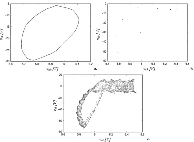
[image:6.594.316.535.417.574.2]Fig. 10. Stroboscopic maps in (a) quasi-periodic (K = 8), (b) subharmonic (K = 23), and (c) chaotic (K = 35) operation.
A. Operation
Symmetrical, periodic, steady-state operation is summa-rized. The controlled switches within one channel are always in complementary states (that is, when is on, is off, and
vice-versa). The commutation times between and are
neglected. The operation of the positive channel is described. By turning on switch , a sinusoidal current pulse
is developed from to in circuit , and (Fig. 7). The capacitor voltage swings from to . By turning on switch at , the choke current commutes from to and is clamped on . The energy stored in the choke at is depleting in the interval . Continuous-conduction mode (CCM) of operation is assumed, that is, the inductor current flows continuously (Fig. 7). To give an insight into the operation, first constant and smooth output voltages and are assumed, although this assumption is dropped in the mathematical description. The inductor current decreases in a linear fashion.
The same process takes place at the negative side, resulting in a negative current pulse and condenser voltage swing after turning on in channel at the beginning of the next half cycle at (Fig. 7). (For interested readers, the time functions of
, and can be found in [13, Fig. 2].)
Note that there are two subperiods in one period and each subperiod has two structures (Figs. 2 and 7). Due to the sym-metrical setup of the two channels, structures 1 and 2 in the two subperiods are the same, and only the active and passive ele-ments might be different, e.g., in place of (in channel ), , and , the corresponding components are (in channel ), , and . Similarly, the state variable belonging
to the elements might change, e.g., replaces in the in-ductor. However, the element and its state variable can be the same in the two subperiods, e.g., switched capacitance and its state variable .
The state equations for structures 1 and 2 of subperiod I are derived in the Appendix. The result in per unit for structure1 [cf. (A2)] is
(35) and for structure 2 [cf. (A4)] is
(36)
where ,
and .
By utilizing the periodicity of the structure series, the values of the five state variables at the end of subperiod , can be transformed back to structure 1 used in subperiod I by the peri-odicity or transfer matrix [Fig. 3]:
[see (9)] Now the same structures (structures 1 and 2) and the same state variables are used even in subperiod II as in subperiod I.
provides the initial condition of the state variables in structure 1 for subperiod II. The result of the back transfor-mation is
Fig. 11. Oscilloscope trace of (a) the condenser voltage and (b) choke current. (A) Period-1 operation,K = 3. (B) Quasi-periodic operation,K = 8. (C) Period-2 operation,K = 13. (D) Chaotic operation,K = 35.
value belonging to at the end of subperiod I (Fig. 7), that is, . Similar statements hold for the other four state variables. We use the same configuration, equations, and state variables in subperiod II as we used in subperiod I but now , and represent the state variables
, and .
The output voltages and currents are exchanged and the sign of is changed in (37). This result can easily be understood from the periodicity of the time functions and from the operation showing that the corresponding time functions in the two chan-nels are the same only they are shifted by to each other. (Fig. 7.) (See the periodicity matrix (A6) in the Appendix.)
VII. RESULTS OF STABILITY ANALYSIS OF
FEEDBACK-CONTROLLEDRESONANTDC–DC CONVERTER A. Simulation and Calculation Results
parameter . The bifurcation diagram is obtained by sampling the switched condenser voltage of the converter at the start of every switching period in the steady state and plotting these sampled values as a function of the bifurcation parameter . The data used are as follows: 125 H; 100 nF; 100 F; 6 8 V;
6 V; 6 V; 6 V. All states have been calcu-lated from the neighboring previous state instead of starting the system from zero initial conditions. On the left side of the bi-furcation diagram, there is just one single sampled value
for a given gain , i.e., the condenser voltage re-peats itself in each switching period and this corresponds to the stable period-1 range (Fig. 8). By increasing , the first bifurcation takes place between and , and it was ana-lyzed with the stability study just presented. However, only the first bifurcation was analyzed in the present paper. Figs. 8, 10, and 11 show further bifurcations and system states contributing significant information about the system behavior in the range of higher values.
Fig. 9 shows the loci of the eigenvalues for the following values of the controller gain: (indicated by ), (indicated by o), and (indicated by x). The stable periodic steady-state solution (all of the eigenvalues lie inside the unit circle) loses stability as the controller gain is increased and generate a quasi-periodic solution, since a complex-conjugate pair of eigenvalues passes through the unit circle at . The eigenvalues were calculated by using the expression of the Jacobian matrix in (27). The pair of eigenvalues at the unit circle is . Note that there are altogether five eigenvalues corresponding to the five energy storage components.
[image:9.594.308.554.577.708.2]The stroboscopic map of the feedback-controlled converter shows the sequence of discrete samples of its arbitrary two state variables taken once in every switching cycle at the interval in the steady state and plotted in the plane of the two variables. Fig. 10 presents the stroboscopic map in quasi-periodic opera-tion [Fig. 10(a), ], in subharmonic operation in period-8 [Fig. 10(b), ], and in chaotic operation [Fig. 10(c),
] in the plane of condenser voltage
versus output voltage . Quasi-periodic opera-tion appears like a closed curve, subharmonic operaopera-tion is rep-resented by eight points, whereas ten chaotic state appears as a set of organized points, reflecting a multilayered structure and order.
B. Test Results
Tests were performed in order to verify the complex dynam-ical behavior revealed by computer simulations and stability study. The presentation includes oscilloscope traces of the con-denser voltage and choke current , for the parameter values specified at the beginning of Section VII. The time function of period-1 operation [Fig. 11(A), ], the quasi-peri-odic operation [Fig. 11(B), ], the subharmonic (pe-riod-2) operation [Fig. 11(C), ] and the chaotic oper-ation [Fig. 11(D), ] are presented. Qualitatively, the measurement results are in good agreement with the simula-tion ones. Quantitatively, there are deviasimula-tions due to the pres-ence of parasitic elements in the practical circuit (ideal
compo-nents were assumed in simulations and in the stability analysis). These discrepancies do not influence the detected phenomena; they only shift the bifurcation points (e.g., the Hopf bifurcation in the experimental circuit occurs at a higher controller gain, about ).
VIII. CONCLUSION
The paper applied conventional tools for the stability anal-ysis of variable-structure piecewise-linear nonlinear feedback systems, namely, the eigenvalues of the Jacobian matrix of the PMF belonging to a fixed point of the system. The paper intro-duced two contributions; the first one is less significant, while the second one is the major contribution. First, it utilized the periodicity of the variable structure and this way it permits the application of the same equations written only for one part of the entire configuration which is continuously repeated after switching actions.
Second, and most important, it determined the Jacobian ma-trix by using the small differences of the state vectors compared to their steady-state values at the start and end of subperiods and at the switching instant. There was no need to determine the derivatives of the PMF at the fixed point. The Jacobian matrix was obtained directly from the relations among the small differ-ences of the state vectors. In addition, all steps were interpreted graphically in Figs. 3 and 4. Consequently, this method offered an alternative way to derive the Jacobian matrix or, which is more significant, a simpler and faster way to determine it. The key element of this method was the introduction of the auxil-iary state vector for preserving constant switching instants for the switchings depending on state variables even after the small excursion of the state variables from the steady state, although in reality it varies a small extent.
In addition, the application of the method was presented in the example of a feedback-controlled resonant dc–dc converter. Simulations, calculations, and test results illustrated the theoret-ical considerations.
APPENDIX
DERIVATION OFSTATEEQUATIONS
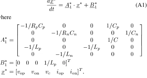
The linear state equations of the structures in subperiod I are as follows (Figs. 5 and 6). For structure 1, we have
(A1) where
Rewriting (A1) in per unit ( , we have
where
and
For structure 2, we have
(A3) where
Rewriting (A3) in per unit yields
(A4)
Utilizing the symmetry and periodicity of the converter on the basis of Figs. 6 and 7, the transfer matrix is
(A5)
ACKNOWLEDGMENT
The authors would like to thank the Hungarian-Romanian In-tergovernmental S & T Cooperation Programme and the HAS and Japanese Society for the Promotion of Science (JSPS) for the support stemming from their cooperation.
REFERENCES
[1] S. Banerjee and G. C. Verghese,Nonlinear Phenomena in Power Elec-tronics. Piscataway, NJ: IEEE Press, 2001.
[2] J. Guckenheimer and P. Holmes, Nonlinear Oscillations, Dy-namical Systems, and Bifurcations of Vector Fields. New York: Springer-Verlag, 1992.
[3] R. C. Hilborn,Chaos and Nonlinear Dynamics. New York: Oxford Univ. Press, 1994.
[4] F. C. Moon,Chaotic and Fractal Dynamics. New York: Wiley, 1992. [5] E. Ott,Chaos in Dynamical Systems. Cambridge, U.K.: Cambridge
Univ. Press, 1997.
[6] M. A. Aizerman and F. R. Gantmakher, “Stability in the linear approxi-mation of the periodic solution of a system of differential equations with discontinuous right-hand part” (in Russian),Prikl. Mat. Mekh., vol. 21, pp. 658–669, 1957.
[7] A. F. Filippov,Differential Equations with Discontinuous Right-Hand Sides. Dordrecht, The Netherlands: Kluwer, 1988.
[8] V. S. Baushevet al., “Local stability of periodic solutions in sample data control systems,” inAutomation and Remote Control. New York: Plenum, 1992, pt. 2, vol. 53, pp. 865–871.
[9] Zh. T. Zhusubaliyev and E. Mosekilde,Bifurcations and Chaos in Piece-wise-Smooth Dynamical Systems, Singapore: World Scientific, 2003. [10] L. Benaderoet al., “Two-dimensional bifurcation diagrams. Background
pattern of fundamental DC-DC converters with PWM control,”Int. J. Bifurc. Chaos, vol. 13, pp. 427–451, 2003.
[11] A. El Aroudi and R. Leyva, “Quasiperiodic route to chaos in a PWM voltage-controlled DC-DC boost converter,”IEEE Trans. Circuits Syst. I, vol. 48, no. 8, pp. 967–978, Aug. 2001.
[12] Y. Kuroe, “Computer algorithm to analyze stability of power electronic systems,” inProc. Power Conversion Conf., Osaka, Japan, Apr. 2–5, 2002, pp. 293–298.
[13] O. Drangaet al., “Stability analysis of a feedback controlled resonant DC-DC converter,”IEEE Trans. Ind. Electron., vol. 50, no. 1, pp. 141–152, Feb. 2003.
[14] H. H. C. Iu and C. K. Tse, “Bifurcation behavior of parallel-connected buck converters,”IEEE Trans. Circuits Syst., vol. 48, no. 2, pp. 233–240, Feb. 2001.
[15] L. Benaderoet al., “Bifurcations analysis in PWM regulated DC-DC converters using averaged models,” inProc. EPE-PEMC’02, Croatia, 2002, Available: [CDRom].
[16] O. Woywode and H. Güldner, “Application of statistical analysis to DC-DC converters,” inProc. Int. Power Electron. Conf., IPEC 2000, Tokyo, Japan, Apr. 2000, pp. 90–94.
[17] C.-C. Fang, “Exact orbital stability analysis of static and dynamic Ramp compensations in DC-DC converters,” inProc. ISIE’2001 Conf., vol. III, Pusan, Korea, 2001, pp. 2124–2129.
[18] A. El Aroudiet al., “Quasiperiodic route to chaos in DC-DC switching regulators,” in Proc. ISIE’2001 Conf., vol. III, Pusan, Korea, pp. 2130–2135.
[19] J. L. R. Marreroet al., “Analysis of the chaotic regime for dc-dc con-verters under current mode control,” inProc. IEEE Power Electron. Spe-cialists Conf., 1996, pp. 1477–1483.
[21] W. C. Y. Chan and C. K. Tse, “Study of bifurcations in current-pro-grammed DC-DC boost converters: From quasiperiodicity to period doubling,”IEEE Trans. Circuits Syst. I, vol. 44, no. 12, pp. 1129–1142, Dec. 1997.
[22] J. H. Chenet al., “Experimental stabilization of chaos in a voltage-mode DC drive system,”IEEE Trans. Circuits Syst. I, vol. 47, no. Jul., pp. 1093–1095, 2000.
[23] I. Rácz, “Calculation of thyristor controlled electric machines with matrix calculus,” inProc. 1st Conf. Power Electron. Motion Control, PEMC’70, Budapest, Hungary, 1970, pp. 2.1.1–2.1.11.
[24] M. Orabi and T. Ninomiya, “Analysis of PFC converter stability using energy balance theory,” inProc. IECON’03. Roanoke, VA, 2003, pp. 544–549.
[25] O. Dranga and I. Nagy, “Stability analysis of feedback controlled reso-nant DC-DC converter using poincare map function,” inProc. ISIE, vol. III, Pusan, Korea, Jun. 12–16, 2001, pp. 2142–2147.
[26] J. Hamar and I. Nagy, “Asymmetrical operation of dual channel resonant DC-DC converters,”IEEE Trans. Power Electron., vol. 18, no. 1, pp. 83–94, Jan. 2003.
Octavian Drangawas born in Romania in 1971. He received the B.Sc., M.Sc., and Ph.D. degrees in control engineering from the “Politechnica” University of Timiooara, Timiooara, Romania in 1995, 1996, and 2001, respectively.
He was with the “Politehnica” University of Timiooara from 1996 to 1998. During 1998–2001, he was a Ph.D. student at the Budapest University of Technology and Economics, Budapest, Hungary. He held postdoctoral research positions with Hong Kong Polytechnic University (2001–2002), Univer-sity of Hull, Hull, U.K. (2003), and Utsunomiya UniverUniver-sity, Tochigi, Japan (2003–2004). He is currently with the Hong Kong Polytechnic University as a Research Fellow. His research interest is in the study of nonlinear phenomena in power electronics. He has authored 40 papers.
Balázs Butiwas born in Berettyóújfalu, Hungary, in 1978. He received the M.Sc. degree from the Budapest University of Technology and Economics, Budapest, Hungary, in 2001, where he is currently working toward the Ph.D. degree.
His research interests focus on power electronics, nonlinear systems, and control systems. He is the coauthor of 15 technical papers.
István Nagy (M’92–SM’99–F’00) received the Ph.D. degree from the Technical University of Budapest, Budapest, Hungary, in 1960.
He has been associated with the Institute of Au-tomation and Computation, Hungarian Academy of Sciences, Budapest, since 1960, where he headed the Department of Power Electronics for 15 years. He be-came a Full Professor with the Technical University of Budapest, Budapest, Hungary, in 1975. He was a Visiting Professor at universities in Sweden, Ger-many, India, New Zealand, Italy, Canada, the U.S., and Japan. His research interests are power electronics, control of ac drives, and nonlinear dynamics. He has authored or coauthored 13 textbooks and approxi-mately 170 technical papers and holds 13 patents.
Prof. Nagy is a member of the Hungarian Academy of Sciences, chairman of EPE-PEMC council, member of the Hungarian IEE and EPE. He is also a member of AdCom of the IES and the IEEE Power Electron Society.
Hirohito Funato (S’93–M’95) was born in Fukushima, Japan, in 1964. He received the B.Eng., M.Eng., and Ph.D. degrees in electrical engineering from Yokohama National University, Yokohama, Japan, in 1987, 1989, and 1995, respectively.