The PID controller design using genetic algorithm

University of Southern Queensland

Faculty of Engineering and Surveying

THE PID CONTROLLER DESIGN USING

GENETIC ALGORITHM

A dissertation submitted by

SAIFUDIN BIN MOHAMED IBRAHIM

in fulfillment of the requirements of

Courses ENG4111 and ENG4112 Research Project

towards the degree of

Bachelor of Engineering (Electrical and Electronics)

Abstract

It is known that PID controller is employed in every facet of industrial automation. The application of PID controller span from small industry to high technology industry. For those who are in heavy industries such as refineries and ship-buildings, working with PID controller is like a routine work. Hence how do we optimize the PID controller? Do we still tune the PID as what we use to for example using the classical technique that have been taught to us like Ziegler-Nichols method? Or do we make use of the power of computing world by tuning the PID in a stochastic manner?

In this dissertation, it is proposed that the controller be tuned using the Genetic Algorithm technique. Genetic Algorithms (GAs) are a stochastic global search method that emulates the process of natural evolution. Genetic Algorithms have been shown to be capable of locating high performance areas in complex domains without experiencing the difficulties associated with high dimensionality or false optima as may occur with gradient decent techniques. Using genetic algorithms to perform the tuning

of the controller will result in the optimum controller being evaluated for the system every time.

The PID controller of the model will be designed using the classical method and the results analyzed. The same model will be redesigned using the GA method. The results of both designs will be compared, analyzed and conclusion will be drawn out of the

University of Southern Queensland

Faculty of Engineering and Surveying

ENG4111 & ENG4112

Research Project

Limitations of Use

The Council of the University of Southern Queensland, its Faculty of Engineering and Surveying, and the staff of the University of Southern Queensland, do not accept any responsibility for the truth, accuracy or completeness of material contained within or associated with this dissertation.

Persons using all or any part of this material do so at their own risk, and not at the risk of the Council of the University of Southern Queensland, its Faculty of Engineering and Surveying or the staff of the University of Southern Queensland.

This dissertation reports an educational exercise and has no purpose or validity beyond this exercise. The sole purpose of the course pair entitled "Research Project" is to contribute to the overall education within the student’s chosen degree program. This document, the associated hardware, software, drawings, and other material set out in the associated appendices should not be used for any other purpose: if they are so used, it is entirely at the risk of the user.

Prof G Baker Dean

Certification of Dissertation

I certify that the ideas, designs an experimental works, analyses and conclusion set out in this dissertation and entirely my own effect, except where otherwise indicated and acknowledged.

I further certify that the work is original and has not been previously submitted for assessment in any other course or other institution, except where specifically stated.

Saifudin bin Mohamed Ibrahim Student Number: D1139088

_________________________ Signature

Acknowledgements

In the name of Allah the most Gracious and most Merciful.

There are a few people that I would like to thank to.

To my supervisor, Dr Paul Wen for giving me valuable feedbacks on how to improve my dissertation.

To Associate Professor Dr John Leis, for advising me against switching to Bachelor of Engineering Technology Degree when it seems impossible for me to complete this course due to family and working commitments. Your kind emails and words had given me motivation to complete the course.

To my ailing father Mohammed Ibrahim, I hope you get well soon and I am looking forward to share this Degree with you.

To my three wonderful children Arina Nadiah, Nurin Nazurah and Muhammad Rusyaidi, I hope you that all of you can take me as an example and quest for knowledge as far as you are able to.

Contents

Abstract vii

Certification Of Dissertation vii

Acknowledgements vii

Lists of Figures vii

Lists of Tables vii

1 Introduction 1

1.1 Project Aims And Objectives. 1

1.2 Background. 2

2 Genetic Algorithm 9

2.1 Introduction. 9

2.2 Characteristics Of GAs. 10

2.3 Population Size. 11

2.4 Reproduction. 12

2.5 Crossover. 14

2.6 Mutation. 16

2.7 Summary Of Genetic Algorithm Process. 18

2.8 Elitism. 19

2.9 Objective Function Or Fitness Function. 19 2.10 Application of GAs in Control Engineering. 20

3 PID Controller 22

3.1 Introduction. 22

3.2 PID Controller. 23

3.3 Continuous PID Control. 24

4 Optimizing of PID Controller 26

4.1 Introduction. 26

4.2 Designing PID Parameters. 27

5 Designing of PID using Genetic Algorithm 45

5.1 Introduction. 45

5.2 Initializing the Population of the Genetic Algorithm. 46

5.3 Setting The GA Parameters. 48

5.4 Performing The Genetic Algorithm. 51

5.5 The Objective Function Of The Genetic Algorithm. 53 5.6 Results Of The Implemented GA PID Controller. 55

6 Further Works And Conclusion 65

6.1 Further Works. 65

6.2 Conclusions. 66

References 68

Appendix A – Project Specification 70

List Of Figures

Figure 1 – Typical Turbine Speed Control.

Figure 2 – Depiction of Roulette Wheel Selection. Figure 3 – Illustration Of Crossover.

Figure 4 – Illustration Of Multi-Point Crossover. Figure 5 – Illustration Of A Uniform Crossover. Figure 6 – Illustration Of Mutation Operation. Figure 7 – Genetic Algorithm Process Flowchart.

Figure 8 – Schematic Of The PID Controller – Non-Interfacing Form. Figure 9 – Block Diagram Of Continuous PID Controller.

Figure 12 – Illustration Of Close Loop Transfer Function. Figure 13 – Simplified System.

Figure 14 – Unit Step Response Of The Designed System Figure 15 – Improved System Response.

Figure 16 – “Optimized” System Response.

Figure 17 – Optimization With Steepest Descent Gradient Method. Figure 18 – Error Signal Of The Optimized System.

Figure 19 – Initialized The GA.

Figure 20 – Parameters Setting Of GA. Figure 21 – Performing The GA.

Figure 22 – Illustration Of Genetic Algorithm Converging Through Generations. Figure 23 – Objective Function.

Figure 24 – Calculating The Error Of The System Using MSE Citeria. Figure 25 –. Stability Of The Controlled System.

Figure 26 – PID Response With Population Size Of 20.

Figure 27 – Analysis Of PID Response With Population Size Of 20. Figure 28 – PID Response With Population Size Of 40.

Figure 29 – Analysis Of PID Response With Population Size Of 40. Figure 30 – Analysis Of PID Response With Population Size Of 60. Figure 31 – PID Response With Population Size Of 80.

Figure 32 – Analysis Of PID Response With Population Size Of 80.

List Of Tables

Table 1 – Routh Array.

Table 2 – Recommended PID Value Setting.

Chapter 1

Introduction

1.1 Project Aims And Objectives

The aim of this project is to design a plant using Genetic Algorithm. What is Genetic Algorithm? Genetic Algorithm or in short GA is a stochastic

algorithm based on principles of natural selection and genetics. Genetic Algorithms (GAs) are a stochastic global search method that mimics the process of natural evolution. Genetic Algorithms have been shown to be capable of locating high performance areas in complex domains without experiencing the difficulties associated with high dimensionality or false optima as may occur with gradient decent techniques. Using genetic

The objective of this project is to show that by employing the GA method of tuning a plant, an optimization can be achieved. This can be seen by

comparing the result of the GA optimized plant against the classically tuned plant.

1.2 Background

In refineries, in chemical plants and other industries the gas turbine

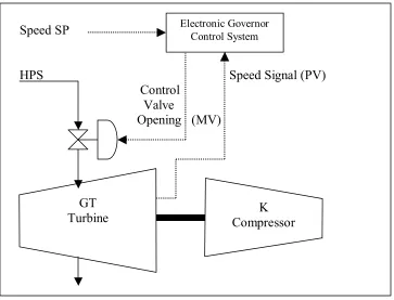
is a well known tool to drive compressors. These compressors are normally of centrifugal type. They consume much power due to the fact that very large volume flows are handled. The combination gas turbine-compressor is highly reliable. Hence the turbine-compressor play significant role in the operation of the plants.

Speed SP

HPS Speed Signal (PV) Control

Valve

Opening (MV)

Figure 1. Typical Turbine Speed Control. GT

Turbine _CompressorK

In the above set up, the high pressure steam (HPS) is usually used to drive the turbine. The turbine which is coupled to the compressor will then drive the compressor. The hydraulic governor which, acts as a control valve will be used to throttle the amount of steam that is going to the turbine section. The governor opening is being controlled by a PID which is in the electronic governor control panel.

It is a known fact that the PID controller is employed in every facet of industrial automation. The application of PID controller span from small industry to high technology industry. For those who are in heavy industries such as refineries and shipbuildings, working with PID controller is like a routine work. Hence how do we optimize the PID controller? Do we still tune the PID as what we use to for example using the classical technique that have been taught to us like Ziegler-Nichols method? Or do we make use of the power of computing world by tuning the PID in a stochastic manner?

In this project, it is proposed that the controller be tuned using the Genetic Algorithm technique. Using genetic algorithms to perform the tuning of the controller will result in the optimum controller being evaluated for the system every time.

as illustrated above in figure 1. The complexities of the electronic governor controller will not be taken into consideration in this dissertation. The electronic governor controller is a big subject by itself and it is beyond the scope of this study.

Nevertheless this study will focus on the model that makes up the steam turbine and the hydraulic governor to control the speed of the turbine.

In the context of refineries, you can consider the steam turbine as the heart of the plant. This is due to the fact that in the refineries, there are lots of high capacities compressors running on steam turbine. Hence this makes the control and the tuning optimization of the steam turbine significant.

During the reproduction phase the fitness value of each chromosome is assessed. This value is used in the selection process to provide bias towards fitter individuals. Just like in natural evolution, a fit chromosome has a higher probability of being selected for reproduction. This continues until the selection criterion has been met. The probability of an individual being selected is thus related to its fitness, ensuring that fitter individuals are more likely to leave offspring. Multiple copies of the same string may be selected for reproduction and the fitter strings should begin to dominate.

Once the selection process is complete, the crossover algorithm is initiated. The crossover operations swaps certain parts of the two selected strings in a bid to capture the good parts of old chromosomes and create better new ones. Genetic operators manipulate the characters of a chromosome directly, using the assumption that certain individual’s gene codes, on average, produce fitter individuals. The crossover probability indicates how often crossover is

performed. A probability of 0% means that the ‘offspring’ will be exact replicas of their ‘parents’ and a probability of 100% means that each generation will be composed of entirely new offspring.

Using selection and crossoveron their own will generate a large amount of different strings. However there are two main problems with this:

2. The GA may converge on sub-optimum strings due to a bad choice of initial population.

These problems may be overcome by the introduction of a mutation operator into the GA. Mutation is the occasional random alteration of a value of a string position. It is considered a background operator in the genetic algorithm The probability of mutation is normally low because a high mutation rate would destroy fit strings and degenerate the genetic algorithm into a random search. Mutation probability values of around 0.1% or 0.01% are common, these values represent the probability that a certain string will be selected for mutation for an example for a probability of 0.1%; one string in one thousand will be selected for mutation. Once a string is selected for mutation, a

randomly chosen element of the string is changed or ‘mutated’.

1.3 Literatures Reviews

Books

□ David E. Goldberg, Genetic Algorithms in Search, Optimization and Machine Learning. The University of Alabama, Addison-Wesley Publishing Company Inc, 1989.

□ John Leis, Digital Signal Processing – A MATLAB-Based Tutorial Approach, University Of Southern Queensland, Research Studies Press Limited, 2002.

□ K. Astrom and T Hagglund, PID Controllers: Theory, Design and Tuning, Prentice Hall, 1984.

□ K Ogata, Discrete-Time Control Systems, University of Minnesota, Prentice Hall, 1987.

Journals

□ T O’Mahony, C J Downing and K Fatla, Genetic Algorithm for PID Parameter Optimization: Minimizing Error Criteria, Process Control and Instrumentation 2000 26-28 July 2000, University of Stracthclyde, pg 148-153.

□ Chipperfield, A. J., Fleming, P. J., Pohlheim, H. and Fonseca, C. M., A Genetic Algorithm Toolbox for MATLAB, Proc. International Conference on Systems Engineering, Coventry, UK, 6-8 September, 1994.

□ Q Wang, P Spronck and R Tracht, An Overview Of Genetic Algorithms

Applied To Control Engineering Problems, Proceedings of the Second International Conference on Machine Learning And Cybernetics, 2003. □ K. Krishnakumar and D. E. Goldberg, Control System Optimization Using

Genetic Algorithms, Journal of Guidance, Control and Dynamics, Vol. 15, No. 3, pp. 735-740, 1992.

□ A. Varsek, T. Urbacic and B. Filipic, Genetic Algorithms in Controller Design and Tuning, IEEE Trans. Sys.Man and Cyber, Vol. 23, No. 5, pp1330-1339, 1993.

“acceptably quickly”. Where specialised techniques exist for solving particular problems, they are likely to out-perform GAs in both speed and accuracy of the final result, so there is no black magic in evolutionary computation. Therefore GAs should be used when there is no other known efficient problem solving strategy.

However in this project, GA is still use as the “preferred” optimized method in optimizing the turbine speed control system. You will see that some other optimization method can be better in certain areas of

Chapter 2

Genetic Algorithm

2.1 Introduction

Genetic Algorithms (GA’s) are a stochastic global search method that mimics the process of natural evolution. It is one of the methods used for optimization. John Holland formally introduced this method in the United States in the 1970 at the University of Michigan. The continuing performance improvements of computational systems has made them attractive for some types of optimization.

as reproduction, crossover and mutation to arrive at the best solution. By starting at several independent points and searching in parallel, the algorithm avoids local minima and converging to sub optimal solutions.

In this way, GAs have been shown to be capable of locating high performance areas in complex domains without experiencing the difficulties associated with high dimensionality, as may occur with gradient decent techniques or methods that rely on derivative information [2].

2.2 Characteristics of Genetic Algorithm

Genetic Algorithms are search and optimization techniques inspired by two biological principles namely the process of “natural selection” and the mechanics of “natural genetics”. GAs manipulate not just one potential solution to a problem but a collection of potential solutions. This is known as population. The potential solution in the population is called “chromosomes”. These chromosomes are the encoded representations of all the parameters of the solution. Each chromosomes is compared to other chromosomes in the population and awarded fitness rating that indicates how successful this chromosomes to the latter.

The selection mechanism for parent chromosomes takes the fitness of the parent into account. This will ensure that the better solution will have a higher chance to procreate and donate their beneficial characteristic to their offspring.

A genetic algorithm is typically initialized with a random population consisting of between 20-100 individuals. This population or also known as mating pool is usually represented by a real-valued number or a binary string called a

chromosome. For illustrative purposes, the rest of this section represents each chromosome as a binary string. How well an individual performs a task is measured and assessed by the objective function. The objective function assigns each individual a corresponding number called its fitness. The fitness of each chromosome is assessed and a survival of the fittest strategy is applied. In this project, the magnitude of the error will be used to assess the fitness of each chromosome.

There are three main stages of a genetic algorithm, these are known as

reproduction, crossover and mutation. This will be explained in details in the following section.

2.3 Population Size

However the matter of the fact is that more and more theories and experiments are conducted and tested and there is no fast and thumb rule with regards to which is the best method to adopt. For a long time the decision on the population size is based on trial and error[6].

In this project the approach in determining the population is rather unsciencetific. From my reading of various papers, it suggested that the safe population size is from 30 to 100. In this project an initial population of 20 were used and the result observed. The result was not promising. Hence an initiative of 40, 60, 80 and 90 size of population were experimented. It was observed that the population of 80 seems to be a good guess. Population of 90 and above does not results in any further optimization.

2.4 Reproduction

During the reproduction phase the fitness value of each chromosome is

assessed. This value is used in the selection process to provide bias towards fitter individuals. Just like in natural evolution, a fit chromosome has a higher

probability of being selected for reproduction. An example of a common selection technique is the ‘Roulette Wheel’ selection method as shown in Figure 2. Each individual in the population is allocated a section of a roulette wheel. The size of the section is proportional to the fitness of the individual.

individuals are more likely to leave offspring.

Multiple copies of the same string may be selected for reproduction and the fitter strings should begin to dominate. However, for the situation illustrated in Figure 8, it is not implausible for the weakest string (01001) to dominate the selection process.

Figure 2. Depiction of roulette wheel selection

There are a number of other selection methods available and it is up to the user to select the appropriate one for each process. All selection methods are based on the same principal that is giving fitter chromosomes a larger probability of selection.

Four common methods for selection are: 1. Roulette Wheel selection

2. Stochastic Universal sampling 3. Normalized geometric selection 4. Tournament selection

Due to the complexities of the other methods, the Roulette Wheel methods is

35% 17%

01110 01001

preferred in this project.

2.5 Crossover

Once the selection process is completed, the crossover algorithm is initiated. The crossover operations swaps certain parts of the two selected strings in a bid to capture the good parts of old chromosomes and create better new ones. Genetic operators manipulate the characters of a chromosome directly, using the

assumption that certain individual’s gene codes, on average, produce fitter

individuals. The crossover probability indicates how often crossover is performed. A probability of 0% means that the ‘offspring’ will be exact replicas of their ‘parents’ and a probability of 100% means that each generation will be composed of entirely new offspring. The simplest crossover technique is the Single Point Crossover.

There are two stages involved in single point crossover:

1. Members of the newly reproduced strings in the mating pool are ‘mated’ (paired) at random.

2. Each pair of strings undergoes a crossover as follows: An integer k is randomly selected between one and the length of the string less one, [1,L-1]. Swapping all the characters between positions k+1 and L inclusively creates two new strings.

Example: If the strings 10000 and 01110 are selected for crossover and the value of k is randomly set to 3 then the newly created strings will be 10010 and 01100

100 00 10010 011 10 01100

Figure 3. Illustration of Crossover.

More complex crossover techniques exist in the form of Multi-point and Uniform Crossover Algorithms. In Multi-point crossover, it is an extension of the single point crossover algorithm and operates on the principle that the parts of a chromosome that contribute most to its fitness might not be adjacent. There are three main stages involved in a Multi-point crossover.

1. Members of the newly reproduced strings in the mating pool are ‘mated’ (paired) at random.

2. Multiple positions are selected randomly with no duplicates and sorted into ascending order.

3. The bits between successive crossover points are exchanged to produce new offspring.

Example: If the string 11111 and 00000 were selected for crossover and the multipoint crossover positions were selected to be 2 and 4 then the newly created strings will be 11001 and 00110 as shown in Figure 4.

11 11 1 11001

00 00 0 00110

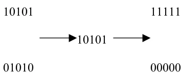
In uniform crossover, a random mask of ones and zeros of the same length as the parent strings is used in a procedure as follows.

1. Members of the newly reproduced strings in the mating pool are ‘mated’ (paired) at random.

2. A mask is placed over each string. If the mask bit is a one, the underlying bit is kept. If the mask bit is a zero then the corresponding bit from the other string is placed in this position.

Example: If the string 10101 and 01010 were selected for crossover with the mask

10101 then newly created strings would be 11111 and 00000 as shown in Figure 5.

10101 11111

10101

01010 00000

Figure 5. Illustration of a Uniform Crossover.

Uniform crossover is the most disruptive of the crossover algorithms and

has the capability to completely dismantle a fit string, rendering it useless in the next generation. Because of this Uniform Crossover will not be used in this project and Multi-Point Crossover is the preferred choice.

2.6 Mutation

1. Depending on the initial population chosen, there may not be enough diversity in the initial strings to ensure the Genetic Algorithm searches the entire problem space.

2. The Genetic Algorithm may converge on sub-optimum strings due to a bad choice of initial population.

These problems may be overcome by the introduction of a mutation operator into the Genetic Algorithm. Mutation is the occasional random alteration of a value of a string position. It is considered a background operator in the genetic algorithm The probability of mutation is normally low because a high mutation rate would destroy fit strings and degenerate the genetic algorithm into a random search. Mutation probability values of around 0.1% or 0.01% are common, these values 55represent the probability that a certain string will be selected for mutation i.e. for a

probability of 0.1%; one string in one thousand will be selected for mutation. Once a string is selected for mutation, a randomly chosen element of the string is changed or ‘mutated’. For example, if the GA chooses bit position 4 for mutation in the binary string 10000, the resulting string is 10010 as the fourth bit in the string is flipped as shown in Figure 6.

10000 10010

2.7 Summary Of Genetic Algorithm Process

In this section the process of Genetic Algorithm will be summarized in a flowchart. The summary of the process will be described below.

Figure 7. Genetic Algorithm Process Flowchart

The steps involved in creating and implementing a genetic algorithm:

1. Generate an initial, random population of individuals for a fixed size. 2. Evaluate their fitness.

3. Select the fittest members of the population. Create/Initialize

Population

Measure/Evaluate Fitness

Select Fittest

Mutation

Crossover / Production

Optimum Solution

4. Reproduce using a probabilistic method (e.g., roulette wheel). 5. Implement crossover operation on the reproduced chromosomes

(choosing probabilistically both the crossover site and the ‘mates’). 6. Execute mutation operation with low probability.

7. Repeat step 2 until a predefined convergence criterion is met.

The convergence criterion of a genetic algorithm is a user-specified condition for example the maximum number of generations or when the string fitness value exceeds a certain threshold.

2.8 Elitism

In the process of the crossover and mutation-taking place, there is high chance that the optimum solution could be lost. There is no guarantee that these operators will preserve the fittest string. To avoid this, the elitist models are often used. In this model, the best individual from a population is saved before any of these operations take place. When a new population is formed and evaluated, this model will examine to see if this best structure has been preserved. If not the saved copy is reinserted into the population. The GA will then continues on as

normal[2].

2.9 Objective Function Or Fitness Function

objective function. This raw measure of fitness is usually only used as an

intermediate stage in determining the relative performance of individuals in a GA.

Another function that is the fitness function, is normally used to transform the objective function value into a measure of relative fitness, thus where f is the objective function, g transforms the value of the objective function to a non- negative number and F is the resulting relative fitness. This mapping is always necessary when the objective function is to be minimized as the lower objective function values correspond to fitter individuals. In many cases, the fitness function value corresponds to the number of offspring that an individual can expect to produce in the next generation. A commonly used transformation is that of proportional fitness assignment[15].

2.10 Application Of Genetic Algorithms In Control Engineering

The following are some GA applications in use control engineering.

• Multiobjective Control.

• PID control.

• Optimal Control.

• Robust Control.

Chapter 3

PID Controller

3.1 Introduction

PID controller consists of Proportional Action, Integral Action and Derivative Action. It is commonly refer to Ziegler-Nichols PID tuning parameters. It is by far the most common control algorithm [1]. In this chapter, the basic concept of the PID controls will be explained.

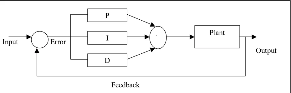
It is interesting to note that more than half of the industrial controllers in use today utilize PID or modified PID control schemes.Below is a simple diagram illustrating the schematic of the PID controller. Such set up is know as non- interacting form or parallel form.

Figure 8. Schematic of The PID Controller – Non-Interacting Form

3.2 PID Controller

In proportional control,

Pterm = KP X Error

It uses proportion of the system error to control the system. In this action an offset is introduced in the system.

In Integral control,

It is proportional to the amount of error in the system. In this action, the I-action will introduce a lag in the system. This will eliminate the offset that was

introduced earlier on by the P-action. Input Error

Output

Feedback P

I

D

Plant

In Derivative control,

It is proportional to the rate of change of the error. In this action, the D-action will introduce a lead in the system. This will eliminate the lag in the system that was introduced by the I-action earlier on.

3.3 Continuous PID

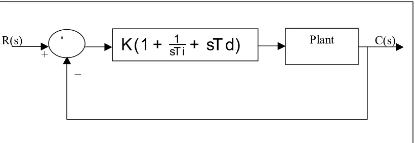
The three controllers when combined together can be represented by the following transfer function.

Gc(s) = K (1 +

+ sTd)

This can be illustrated below in the following block diagram

Figure 9. Block diagram of Continuous PID Controller.

What the PID controller does is basically is to act on the variable to be

manipulated through a proper combination of the three control actions that is the P control action, I control action and D control action.

R(s) C(s) +

_

P _Plant

The P action is the control action that is proportional to the actuating error signal, which is the difference between the input and the feedback signal. The I action is the control action which is proportional to the integral of the actuating error signal. Finally the D action is the control action which is proportional to the derivative of the actuating error signal.

Chapter 4

Optimizing Of PID Controller

4.1 Introduction

For the system under study, Zieger-Nichols tuning rule based on critical gain Ker and critical period Per will be used. In this method, the integral time Ti will be set to infinity and the derivative time Td to zero. This is used to get the initial PID setting of the system. This PID setting will then be further optimized using the “steepest descent gradient method”.

In this chapter, it will be shown that the inefficiency of designing PID controller using the classical method. This design will be further improved by the

optimization method such as “steepest descent gradient method” as mentioned earlier [16].

4.2 Designing PID Parameters

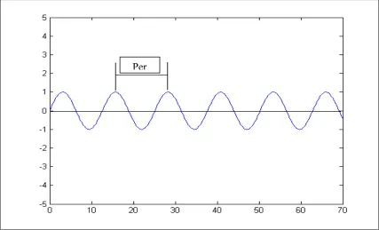
From the response below, the system under study is indeed oscillatory and hence the Z-N tuning rule based on critical gain Ker and critical period Per can be applied.

The transfer function of the PID controller is

G

(s) = K

(1 +

+ T

s )

The objective is to achieve a unit-step response curve of the designed system that exhibits a maximum overshoot of 25 %. If the maximum overshoot is excessive says about greater than 40%, fine tuning should be done to reduce it to less than 25%.

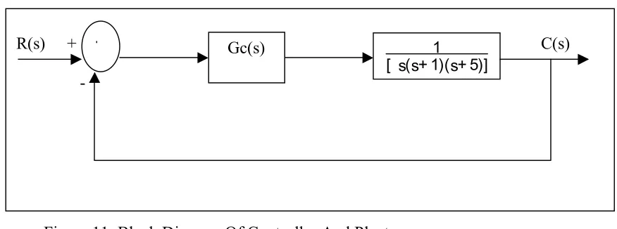
The system under study above has a following block diagram

Figure 11. Block Diagram Of Controller And Plant.

Since the Ti = ∞ and Td = 0, this can be reduced to the transfer function of

R(s) C(s)

=

The value of Kp that makes the system marginally stable so that sustained oscillation occurs can be obtained by using the Routh’s stability citerion. Since the characteristic equation for the closed-loop system is

s

+ 6s

+ 5s+ Kp = 0

From the Routh’s Stability Criterion, the value of Kp that makes the system marginally stable can be determined.

R(s) + C(s) -

P

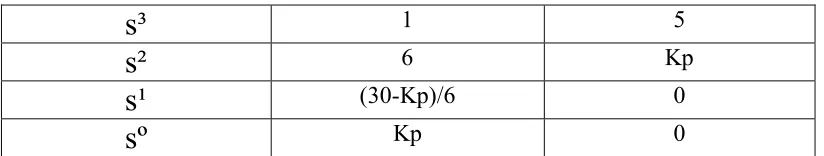
The table below illustrates the Routh array.

s³

s²

s¹

sº

Table 1. Routh Array

By observing the coefficient of the first column, the sustained oscillation will occur if Kp=30.

Hence the critical gain Ker is Ker = 30

Thus with Kp set equal to Ker, the characteristic equation becomes s³ + 6s² + 5s + 30 = 0

The frequency of the sustained oscillation can be determined by substituting the s terms with j_ω term. Hence the new equation becomes

( jω )³ + 6 ( jω )² +5 ( jω ) + 30 = 0 This can be simplified to

6 ( 5 – _ω)² + j_ω ( 5 – _ω ) = 0

From the above simplification, the sustained oscillation can be reduced to

ω² = 5 or

ω = √5

The period of the sustained oscillation can be calculated as Per = 2π/√5

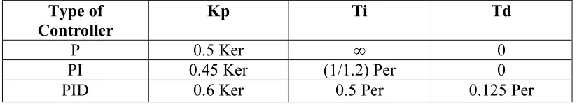
From Ziegler-Nichols frequency method of the second method [1], the table suggested tuning rule according to the formula shown. From these we are able to estimate the parameters of Kp, Ti and Td.

Type of Controller

Kp Ti Td

P 0.5 Ker ∞ 0

PI 0.45 Ker (1/1.2) Per 0

PID 0.6 Ker 0.5 Per 0.125 Per

Table 2. Recommended PID Value Setting.

Hence from the above table, the values of the PID parameters Kp, Ti and Td will

be Kp = 30

Ti = 0.5 X 2.8099 = 1.405

Td = 0.125 X 2.8099 = 0.351.

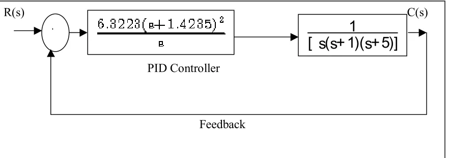
The transfer function of the PID controller with all the parameters is given as

Figure 12. Illustrated the Close Loop Transfer Function.

Using the MATLAB function, the following system can be easily calculated. The above system can be reduced to single block by using the following MATLAB function. Below is the Matlab codes that will calculate the two blocks in series.

% calculation of series system response using matlab num1=[0 6.3223 17.999 12.8089];

den1=[0 0 1 0]; num2=[0 0 0 1]; den2=[1 6 5 0];

[num,den]=series(num1,den1,num2,den2); printsys(num,den)

This will gives the following answer num/den =

6.3223 s^2 + 17.999 s + 12.8089 ---

s^4 + 6 s^3 + 5 s^2

R(s) C(s)

PID Controller

Feedback

P

Hence the above block diagram is reduced to

R(s) C(s)

Figure 13. Simplified System.

Using another MATLAB function, the overall function with its feedback can be calculated as follow

% calculation of feedback system response using matlab num1=[0 0 6.3223 17.999 12.8089];

den1=[1 6 5 0 0]; num2=[0 0 0 0 1]; den2=[0 0 0 0 1];

[num,den]=feedback(num1,den1,num2,den2); printsys(num,den)

This will result to num/den =

6.3223 s^2 + 17.999 s + 12.8089 ---

s^4 + 6 s^3 + 11.3223 s^2 + 17.999 s + 12.8089 Therefore the overall close loop system response of

The unit step response of this system can be obtained with MATLAB.

Figure 14. Unit Step Response Of The Designed System.

The figure above is the system response of the designed system. From the above response it is obvious that the system can be further improved.

%MATLAB script of the Designed PID Controller System. num=[0 0 6.3223 18 12.8];

den=[1 6 11.3223 18 12.811]; step(num,den);

grid;

4.3 Analysis Of The Classically Designed Controller

From the above diagram, we can analyze the response of the system. The zero and pole of the system can be calculated using the MATLAB function “tf2zp”. We can analyze them via the following parameters:

• Delay time, td

• Rise time, tr

• Peak time, tp

• Maximum Overshoot, Mp

• Settling time, ts

The delay time, tdof the above system which is the time taken to reach 50% of the final response time is about 0.5 sec.

The rise time, tr is the time taken to reach 5 to 95 % of the final value is about 1.75 sec.

The Peak time, tp is the time taken for the system to reach the first peak of overshoot is about 2.0 sec.

The Maximum Overshoot, Mp of the system is approximately 60%.

Finally the Settling time, ts is about 10.2 sec. From the analysis above, the system has not been tuned to its optimum. Here we can improve the system by looking into the system zero and pole.

% calculation of zero and pole of the system response using matlab num=[0 0 6.3223 17.999 12.8089];

den=[1 6 11.3223 17.009 12.8089]; [z,p,k]=tf2zp(num,den)

Results: z = -1.4387 -1.4282 p =

-4.0478 -0.3532 + 1.5542i -0.3532 - 1.5542i -1.2457 k =

6.3223

The above result shows that the system is stable since all the poles are located on the left side of the s-plane.

To optimize the response further, the PID controller transfer function must be revisited.

The transfer function of the designed PID controller is

The new PID controller will have the following parameters.

The PID transfer function and plant transfer function in series can be calculated by Matlab and the result as follow,

The total response with a unity feedback can be calculated as follow

The response of the above system can be illustrated in the following plot.

The new system response has somehow improved. The Maximum Overshoot, Mp has reduced to approximately 18%.The Settling Time, ts has improved from 14 sec to 6 sec. The Peak Time, tp and Delay Time, td has increased. The final amplitude has improved at the expense of the system time. The new PID parameters can be calculated as are Kp = 18, Ti = 3.077 and Td = 0.7692.

To improve the system further, lets increase the Kp value to 39.42. The location of double zero will be kept the same i.e s = -0.65. The new transfer function of the PID controller will be

Using the Matlab command, the above function together with the plant transfer function and the unity feedback can be determined. The result is

Figure 16. “Optimized” System Response.

The above response shows that the system has improved. The response is faster than the one shown in figure 15. The Maximum Overshoot, Mp has increased to about 22%. This is still acceptable since the Maximum Overshoot allowable is less than 25%.The Settling Time, ts remain the same i.e. 6 sec. The Peak Time, tp and Delay Time, td has improved. The new PID parameters can be calculated as Kp = 39.42, Ti = 3.077 and Td = 0.7692.

the 25% Maximum Overshoot allowable. The settling time, ts of the second and the third responses fared much better than the first response. The ts reached its steady-state in much faster than the original time taken by the original response.

It is interesting to observe that these values are approximately twice the values suggested by the second method of Z-N tuning rule. Hence we can conclude that Z-N tuning rule has provided us a starting point for a finer tuning.

It is observed that for the case where the double zero is located at s = -1.425, increasing the value of Kp increases the speed of the response. However this does not improve the percentage maximum overshoot. In fact varying Kp has little impact on the percentage maximum overshoot. On the other hand, varying the double zero has significant effect on the maximum overshoot. The zero is shifted form –1.425 to –0.65 and we observed that the maximum overshoot reduces. Finally to achieve a better result, we have to have to double the Kp value coupled with the new zero value and hence the better percentage maximum overshoot can be achieved. The above can explained through the root-locus analysis. The system described above can be further improved or optimized. In the following section, the optimization method used will be discussed.

4.4 Optimizing Of The Designed PID Controller.

The optimizing method used for the designed PID controller is the “steepest gradient descent method”. In this method, we will derived the transfer function of the controller as

The minimizing of the error function of the chosen problem can be achieved if the suitable values of can be determined. These three combinations of

potential values form a three dimensional space. The error function will form some contour within the space. This contour has maxima, minima and gradients which result in a continuous surface.

The idea of this optimization method is reach the minima by the shortest path. In order to achieve this shortest path, moving down the steepest gradient will lead to reaching the minima the soonest. When the gradient changes from point to point, to ensure that the steepest path is still being used, it is significant to choose a new direction and make changes accordingly. Hence the minimization of the error function is achieved by analyzing the function of the function itself. In the next paragraph, the derivation of the plant transfer function to the minimizing of error function will be shown.

Let

Lets B1= q0

B2= q1

B3= q2

B4= (1 + A)

B5= (A + B)

B6= B

Therefore

=

Therefore,

.

Lets D = (2 + B1)

Therefore the difference equation of the optimized PID controller is,

The above equation can be implemented with MATLAB and the response observed. The details of the Matlab codes can be seen in the appendix.

From the plot below we can see the optimization response. In this plot we can see how the optimized controller behave. It can be seen that the curve behaves as if it climbing up the hill. It will improve its performance until there is little error exist and finally it will reach the final value.

Figure 17. Optimization With Steepest Descent Gradient Method In this method, the system is further optimized using the said method. With the “steepest descent gradient method”, the response has definitely improved as compared to the one in Figure 16. The settling time has improved to 2.5 second as compared to 6.0 seconds previously. The setback is that the rise time and the maximum overshoot cannot be calculated. This is due to the “hill climbing” action of the steepest descent gradient method. However this setback was replaced with the quick settling time achieved.

As the error was minimized, the system is reaching its stability.

Figure 18. Error Signal Of The Optimized System

Chapter 5

Designing Of PID

Using Genetic Algorithm

5.1 Introduction

Before we go into the above subject. It is good to discuss the differences between Genetics Algorithm against the traditional methods. This will help us understand why GA is more efficient than the latter. Genetic algorithms are substantially different to the more traditional search and optimization techniques. The five main differences are:

1. Genetic algorithms search a population of points in parallel, not from a single point.

influence the direction of the search.

3. Genetic algorithms use probabilistic transition rules, not deterministic rules.

4. Genetic algorithms work on an encoding of a parameter set not the parameter set itself (except where real-valued individuals are used). 5. Genetic algorithms may provide a number of potential solutions to a given

problem and the choice of the final is left up to the user.

5.2 Initializing the Population of the Genetic Algorithm

The Genetic Algorithm has to be initialized before the algorithm can proceed. The Initialization of the population size, variable bounds and the evaluation function are required. These are the initial input that are required in order for the Genetic Algorithm process to start.

%Initialising the genetic algorithm populationSize=80;

variableBounds=[-100 100;-100 100;-100 100]; evalFN='PID_objfun_MSE';

%Change this to relevant object function evalOps=[];

options=[1e-6 1];

initPop=initializega(populationSize,variableBounds,evalFN… evalOps,options)

Figure 19. Initialize The GA.

The following codes are used to initialize the GA. The codes will be explained in details.

• PopulationSize - The first stage of writing a Genetic Algorithm is to create a population. This command defines the population size of the GA. Generally the bigger the population size the better is the final approximation.

• VariableBounds - Since this project is using genetic algorithms to optimize the gains of a PID controller there are going to be three strings assigned to each member of the population, these members will be comprised of a P, I and a D string that will be evaluated throughout the course of the GA processes. The three terms are entered into the genetic algorithm via the declaration of a three-row

• EvalFN - The evaluation function is the matlab function used to declare the

objective function. It will fetch the file name of the objective function and execute the codes and return the values back to the main codes.

• Options - Although the previous examples in this section were all binary encoded, this was just for illustrative purposes. Binary strings have two main drawbacks:

1. They take longer to evaluate due to the fact they have to be converted

to and from binary.

2. Binary strings will lose its precision during the conversion process.

As a result of this and the fact that they use less memory, real (floating point) numbers will be used to encode the population. This is signified in the options command in Figure 19, where the ‘1e-6’ term is the floating point precision and the ‘1’ term indicates that real numbers are being used (0 indicates binary encoding is being used).

• Initialisega – This command is from the GAOT toolbox. It will combines all the previously described terms and creates an initial population of 80 real valued members between –100 and 100 with 6 decimal place precision.

5.3 Setting The GA Parameters

%Setting the parameters for the genetic algorithm bounds=[-100 100;-100 100;-100 100];

evalFN='PID_objfun_MSE';%change this to relevant object function evalOps=[];

startPop=initPop; opts=[1e-6 1 0];

termFN='maxGenTerm'; termOps=100;

selectFN='normGeomSelect'; selectOps=0.08;

xOverFNs='arithXover'; xOverOps=4;

mutFNs='unifMutation'; mutOps=8;

Figure 20. Parameters Setting Of GA.

• Bounds - The variable bound are for the genetic algorithm to search within a specified area. These bounds may be different from the ones used to initialise the population and they define the entire search space for the genetic algorithm.

• startPop - The starting population of the GA, ‘startPop’, is defined as the population described in the previous section, i.e. ‘initPop’, see Figure 19.

• opts - The options for the Genetic Algorithm consist of the precision of the string values i.e. 1e-6, the declaration of real coded values, 1, and a request for the progress of the GA to be displayed, 1, or suppressed, 0.

criterion of the genetic algorithm when compared with other termination criteria e.g. convergence termination criterion.

• TermOps - This command defines the options, if any, for the termination function. In this example the termination options are set to 100, which means that the GA will reproduce one hundred generations before terminating. This number may be altered to best suit the convergence criteria of the genetic algorithm i.e. if the GA converges quickly then the termination options should be reduced.

• SelectFN - Normalised geometric selection (‘normGeomSelect’) is the primary selection process to be used in this project. The GAOT toolbox provides two other selection functions, Tournament selection and Roulette wheel selection. Tournament selection has a longer compilation time than the rest and as the overall run time of the genetic algorithm is an issue, tournament selection will not be used. The roulette wheel option is inappropriate due to the reasons mentioned in section 2.4.

• SelectOps - When using the ‘normGeomSelect’ option, the only parameter that has to be declared is the probability of selecting the fittest chromosome of each generation, in this example this probability is set to 0.08.

one. This increases the compilation time of the program and is undesirable. The Arithmetic crossover procedure is specifically used for floating point numbers and is the ideal crossover option for use in this project.

• XOverOptions -This is where the number of crossover points is specified.

• mutFNs - The ‘multiNonUnifMutation’, or multi non-uniformly distributed mutation operator, was chosen as the mutation operator as it is considered to function well with multiple variables.

• MutOps - The mutation operator takes in three options when using the ‘multiNonUnifMutation’ function. The first is the total number of mutations, normally set with a probability of around 0.1%. The second parameter is the maximum number of generations and the third parameter is the shape of the distribution. This last parameter is set to a value of two, three or four where the number reflects the variance of the distribution.

5.4 Performing The Genetic Algorithm

The genetic algorithm is compiled using the command shown in Figure .

The function “ga.m” will evaluate and iterate the genetic algorithm until it fulfils the criteria described by its termination function.

%Performing the genetic algorithm

[x,endPop,bPop,traceInfo]=ga(bounds,evalFN,evalOps,startPop,opts,... termFN,termOps,selectFN,selectOps,xOverFNs,xOverOps,mutFNs,mutOps);

Once the genetic algorithm is completed, the above function will return four variables:

x = The best population found during the GA. endPop = The GA’s final population.

bestPop = The GA’s best solution tracked over generations. traceInfo = The best value and average value for each generation.

The best population may be plotted to give an insight into how the genetic Algorithm converged to its final values as illustrated in Figure 22.

5.5 The Objective Function Of The Genetic Algorithm

This is the most challenging part of creating a genetic algorithm is writing the the objective function.. In this project, the objective function is required to evaluate the best PID controller for the system. An objective function could be created to find a PID controller that gives the smallest overshoot, fastest rise time or quickest settling time. However in order to combine all of these objectives it was decided to design an objective function that will minimize the error of the controlled system instead. Each chromosome in the population is passed into the objective function one at a time. The chromosome is then evaluated and assigned a number to represent its fitness, the bigger its number the better its fitness. The genetic algorithm uses the chromosome’s fitness value to create a new population consisting of the fittest members. Below are the codes for the Objective Function.

function [x_pop, fx_val]=PID_objfun_MSE(x_pop,options) global sys_controlled

global time global sysrl

% Splitting the chromosones into 3 separate strings. Kp=x_pop(2);

Ki=x_pop(3); Kd=x_pop(1);

%creating the PID controller from current values pid_den=[1 0];

pid_num=[Kd Kp Ki];

Each chromosome consists of three separate strings constituting a P, I and D term, as defined by the 3-row ‘bounds’ declaration when creating the population. When the chromosome enters the evaluation function, it is split up into its three Terms. The P, I and D gains are used to create a PID controller according to the equation below.

C

=

ps + KI

The newly formed PID controller is placed in a unity feedback loop with the system transfer function. This will result in a reduce of the compilation time of the program. The system transfer function is defined in another file and imported as a global variable. The controlled system is then given a step input and the error is assessed using an error performance criterion such as Mean Square Error or in short MSE. The MSE is an accepted measure of control and of quality but its practical use as a measure of quality is somehow limited [4]. The chromosome is assigned an overall fitness value according to the magnitude of the error, the smaller the error the larger the fitness value. Below is the codes used to implement the MSE performance citeria.

%Calculating the error for i=1:301

error(i) = 1-y(i); end

%Calculating the MSE error_sq = error*error';

MSE=error_sq/max(size(error));

Additional code was added to ensure that the genetic algorithm converges to a controller that produces a stable system. The code, shown in Figure 25, assesses the poles of the controlled system and if they are found to be unstable that is on the right half of the s-plane, the error is assigned an extremely large value to make sure that the chromosome is not reselected.

%Ensuring controlled system is stable poles=pole(sys_controlled);

if poles(1)>0 MSE=100e300; elseif poles(2)>0 MSE=100e300; elseif poles(3)>0 MSE=100e300; elseif poles(4)>0 MSE=100e300; elseif poles(5)>0 MSE=100e300; end

fx_val=1/MSE;

Figure 25. Stability Of The Controlled System.

5.6 Results Of The Implemented Genetic Algorithm PID Controller

From the following responses, the GA designed PID will be compared to the Steepest Descent Gradient Method. The superiority of GA against the SDG method will be shown.

The following is the plot of the GA designed PID with the population size of 20. From the figure below, the response of the GA PID will be analyzed.

Figure 26. PID Response With Population Size Of 20.

Figure 27. Analysis Of PID Response With Population Size Of 20. From the above figure , the details of the system response will be analyzed. The peak amplitude of the response is 1.11. The overshoot of the response is 10.6%. The settling time of the response is 6.97 seconds and finally the response of the rise time is 0.666 seconds.

From one look, the above response is definitely much better than the classical PID tuning method as shown in the chapter 4. However how does it fare against the one optimized using the Steepest Descent Gradient Method? This will be answered after we analyzed the following responses.

Settling Time Max Overshoot

The following figure depict the response of GA designed PID with the population size of 40.

Figure 28. PID Response With Population Size Of 40.

Figure 29. Analysis Of PID Response With Population Size Of 40. From the above figure, the details of the response will be analyzed. The peak amplitude of the response is 1.07. The overshoot of the response is 6.98%. The settling time of the response is 2.2 seconds and the rise time of 0.64 seconds. From the following results, it is obvious that the population of size 40 has returned a better results than the one with the population size of 20.

In this response, the overshoot value has improved. The settling time has reduced from 6.97 seconds to 2.2 seconds. The rise time has improved slightly that is 0.64 seconds as compared to 0.666 seconds. The overall response is that it has

Figure 32. Analysis Of PID Response With Population Size Of 80. The GA designed PID with population size of 80 has the following response factors. The Peak Amplitude of 1.05. Overshoot of 4.86%. Rise time of 0.592 seconds. Settling time of 1.66 seconds.

The following plot will show that the GA designed PID performed better than the Steepest Descent Gradient Method (SDGM).

Figure 33. Response Of GA Designed PID Versus Steepest Descent Optimization Method.

The above analysis is summarized in the following table. Measuring Factors SDGM

Controller

GA Controller Percentage Improvement

Rise Time (sec) 1.0 0.592 40.8 %

Maximum Overshoot (%) NA 4.8 NA

Settling Time (sec) 2.5 1.66 33.6 %

Table 3. Results Of SDGM Designed Controller And GA Designed Controller. From table 3, we can see that the GA designed controller has a significant improvement over the SDGM designed controller. On average the percentage improvement of GA controller against SDGM controller range from 30 % to

GA Response

Chapter 6

Further Works And Conclusions

6.1 Further Works

It is hope that this project can be improved to include the implementation of tuning the PID controller via GA in an online environment. This will have much impact in the optimization of the system under control .

As for the subject under study, if the plant or the turbine system can be tuned using GA in an online environment, there will be minimum losses on the process. The steam used to drive the turbine will be fully utilized and the energy

transferred maximized. There will be minimum loss since the response shown above is as close to the unit step. Hence in the refineries, this will translate to better profit margin.

It is also hope that in the future works, the system to be tested with other Performance Criterion such as IAE, ITAE and ISE. In the current work, due to time constraint, only MSE as the Performance Citerion was implemented. Hence it was not known and proven that the MSE will result a better fitness function measurement.

6.2 Conclusions

In conclusion the responses as shown in chapter 5, had showed to us that the designed PID with GA has much faster response than using the classical method. The classical method is good for giving us as the starting point of what are the PID values. However as shown in chapter 4, the approached in deriving the initial PID values using classical method is rather troublesome. There are many steps and also by trial and error in getting the PID values before you can narrow down in getting close to the “optimized” values.

An optimized algorithm was implemented in the system to see and study how the system response is. This was achieved through implementing the steepest descent gradient method. The results was good but as was shown in Table 3 and

Figure 33. However the GA designed PID is much better in terms of the rise time and the settling time. The steepest descent gradient method has no overshoot but due to its nature of “hill climbing”, it suffers in terms of rise time and settling time.

GA. This is not a positive point if you are to implement this method in an online environment. It only means that the SDGM uses more memory spaces and hence take up more time to reach the peak.

This project has exposed me to various PID control strategies. It has increased my knowledge in Control Engineering and Genetic Algorithm in specific. It has also shown me that there are numerous methods of PID tunings available in the academics and industrial fields. Previously I was comfortable with Z-N classical methods but now I would like to venture into others methods available [9]. However this depends on the opportunity in my work place.

References

[1] Astrom, K., T. Hagglund, “PID Controllers; Theory, Design and Tuning”, Instrument Society of America, Research Triangle Park, 1995.

[2] Goldberg, David E. “Genetic Algorithms in Search, Optimization and Machine Learning”Addison-Wesley Pub. Co. 1989.

[3] Chris Houck, Jeff Joines, and Mike Kay, "A Genetic Algorithm for Function Optimization: A Matlab Implementation" NCSU-IE TR 95-09, 1995.

http://www.ie.ncsu.edu/mirage/GAToolBox/gaot/

[4] G.J. Battaglia and J.M. Maynard, ‘‘Mean square Error: A Useful Tool for Statistical Process Management,’’AMP J. Technol. 2, 47-55, 1992.

[5] Q.Wang, P.Spronck & R.Tracht, “ An Overview Of Genetic Algorithms Applied To Control Engineering Problems,” Proceedings of the Second Conference on Machine Learning and Cybernetics, 2003.

[6] Luke,S., Balan, G.C. and Panait, L, “Population Implosion In Genetic Programming”, Department Of Computer Science, George Mason University.

http://www.cs.gmu.edu/~eclab

[7] Gotshall,S. and Rylander, B., “Optimal Population Size And The Genetic Algoithm.”, Proc On Genetic And Evolutionary Computation Conference, 2000.

[8] Naeem, W., Sutton, R. Chudley. J, Dalgleish, F.R. and Tetlow, S., “ An Online Genetic Algorithm Based Model Predictive Control Autopilot Design With Experimental Verification.” International Journal Of Control, Vol 78, No. 14, pg 1076 – 1090, September 2005.

[10] Herrero, J.M., Blasco, X, Martinez, M and Salcedo, J.V., “Optimal PID Tuning With Genetic Algorithm For Non Linear Process Models.” , 15th Triennial World Congress, 2002.

[11] O’Dwyer, A. “PI And PID Controller Tuning Rules For Time Delay Process: A Summary. Part 1: PI Controller Tuning Rules.” , Proceedings Of Irish Signals And Systems Conference, June 1999.

[12] K. Krishnakumar and D. E. Goldberg, “Control System Optimization Using Genetic Algorithms”, Journal of Guidance, Control and Dynamics, Vol. 15, No. 3, pp. 735-740, 1992.

[13] T O’Mahony, C J Downing and K Fatla, “Genetic Algorithm for PID Parameter Optimization: Minimizing Error Criteria”, Process Control and Instrumentation 2000 26-28 July 2000, University of Stracthclyde, pg 148-153, July 2000.

[14] A. Varsek, T. Urbacic and B. Filipic, “Genetic Algorithms in Controller Design and Tuning”, IEEE Trans. Sys.Man and Cyber, Vol. 23, No. 5, pp1330-1339, 1993.

[15] Chipperfield, A. J., Fleming, P. J., Pohlheim, H. and Fonseca, C. M., “A Genetic Algorithm Toolbox for MATLAB ”, Proc. International Conference on Systems Engineering, Coventry, UK, 6-8 September, 1994.

Appendix 2

format long e

M = 1601; %number of samples taken starting from nT=0 T = 0.0025; %in second

r = ones(1,M); %Unit step signal q0 = 0.001;

q1 = -q0; q2 = 0;

initial_q = [q0 q1 q2];

s_old = []; %store the value of s delta_q = 0.00009;

gamma = 0.005; %step length number_of_trial = 51;

for index = 1:1:number_of_trial,

%Finding S

[k,e] = e_function(T,q0,q1,q2,r);

s = abs(e)*k'; %absolute value of matrix e multiply %with transpose of matrix k

%Finding S_q0

[k,e] = e_function(T,(q0+delta_q),q1,q2,r); s_q0 = abs(e)*k';

%Finding S_q1

[k,e] = e_function(T,q0,(q1+delta_q),q2,r); s_q1 = abs(e)*k';

%Finding S_q2

[k,e] = e_function(T,q0,q1,(q2+delta_q),r); s_q2 = abs(e)*k';

grad_of_s_due_to_q0 = (s_q0-s)/delta_q; grad_of_s_due_to_q1 = (s_q1-s)/delta_q; grad_of_s_due_to_q2 = (s_q2-s)/delta_q;

delta = sqrt(grad_of_s_due_to_q0^2+... grad_of_s_due_to_q1^2+...

grad_of_s_due_to_q2^2);

q0_old = q0; q1_old = q1; q2_old = q2;

if index < number_of_trial, s_old = s;

end

q0 = q0 - constant_p * grad_of_s_due_to_q0; q1 = q1 - constant_p * grad_of_s_due_to_q1; q2 = q2 - constant_p * grad_of_s_due_to_q2;

end

save try_step initial_q q0 q1 q2 T r index delta_q gamma save try_step_backcopy initial_q q0_old q1_old q2_old s_old

save try_step_backcopy q0 q1 q2 s T r index delta_q gamma -append

disp('Previous value q0 q1 q2 s') [q0_old,q1_old,q2_old,s_old] disp('Latest value q0 q1 q2 s') [q0,q1,q2,s]

[k,e] = e_function(T,q0,q1,q2,r); c = r - e;

plot(k,e)

xlabel('time(nT)'),ylabel('e(nT)') title('Error signal,e(nT)')

figure(1);

plot(k,c)

xlabel('time(nT)'),ylabel('c(nT)') title('Output signal,c(nT)')

figure(2);

E_Function.m

function [k,e]=e_function(T,q0,q1,q2,r)

%E_FUNCTION Calculate the error signal, e(nT) in a closed loop system %

% The format is given as [k,e]=e_function(T,q0,q1,q2,r) %

% r is the input signal which starts from nT = 0.

% Since the E_FUNCTION is derived using 'nT', r should be a % function of 'nT'.

%

% T is the sample period.

% q0, q1, q2, are the parameters of a digital PID % controller.

% E_FUNCTION returns the error ouput, e and matrix k which % contains [0 T 2T 3T ...].

%Check the number of input arguments if nargin < 5,

error('The number of input arguments is less than 5.'); end

%Check the number of output arguments if nargout < 2,

error('The number of output arguments is less than 2.'); end

A = 2*exp(-5*T)+1+exp(-T); B = exp(-5*T)+exp(-6*T);

B1 = q0; B2 = q1; B3 = q2; B4 = (1+A); B5 = (A+B); B6 = B;

D=2+B1;

[n,M] = size(r);

signal_r = r; %Make a copy of signal r(nT)

r = [0 0 0 0]; %r(1) point to r(nT); %r(2) point to r(nT-T); %r(3) point to r(nT-2T); %r(4) point to r(nT-3T);

e_temp = [0 0 0 0 ]; %e_temp(1) point to e(nT); %e_temp(2) point to e(nT-T); %e_temp(3) point to e(nT-2T); %e_temp(4) point to e(nT-3T);

r(1) = signal_r(k);

e_temp(1) = (2/D)*r(1)+(B4/D)*r(2)+(B5/