Scalar Transport over Forested Hills

White Rose Research Online

eprints@whiterose.ac.uk

Universities of Leeds, Sheffield and York

http://eprints.whiterose.ac.uk/

This is the author’s post-print version of an article published in

Boundary-Layer

Meteorology, 141 (2)

White Rose Research Online URL for this paper:

http://eprints.whiterose.ac.uk/id/eprint/76544

Published article:

Ross, AN (2011)

Scalar Transport over Forested Hills.

Boundary-Layer

Meteorology, 141 (2). 179 - 199. ISSN 0006-8314

(will be inserted by the editor)

Scalar transport over forested hills

Andrew N. Ross

Received:

Abstract Numerical simulations of scalar transport in neutral flow over forested

ridges are performed using both a one-and-a-half order mixing length closure scheme

and a large-eddy simulation (LES). Such scalar transport (particularly of CO2) has

been a significant motivation for dynamical studies of forest canopy - atmosphere

interactions. Results from the one-and-a-half order mixing length simulations show

that hills where there is significant mean flow into and out of the canopy are more

effi-cient at transporting scalars from the canopy to the boundary layer above. For the case

with a source in the canopy this leads to lower mean concentrations of tracer within

the canopy, although they can be very large horizontal variations over the hill. These

A.N. Ross

Institute for Climate and Atmospheric Science, School of Earth and Environment, University of Leeds,

UK.

Tel.: +44-113-3437590

Fax.: +44-113-3435259

variations are closed linked to flow separation and recirculation in the canopy and can

lead to maximum concentrations near the separation point which exceed those over

flat ground. Simple scaling arguments building on the analytical model of Finnigan

and Belcher (2004, Q. J. Royal Meteorol. Soc. 130:1-29) successfully predict the

vari-ations in scalar concentration near canopy top over a range of hills. Interestingly this

analysis suggests that variations in the components of the turbulent transport term,

rather than advection, give rise to the leading order variations in scalar concentration.

The scaling arguments provide a quantitative measure of the role of advection, and

suggest that for smaller / steep hills and deeper / sparser canopies advection will be

more important. This agrees well with results from the numerical simulations.

A LES is used to support the results from the mixing-length closure model and

to allow more detailed investigation of the turbulent transport of scalars within and

above the canopy. Scalar concentration profiles are very similar in both models,

de-spite the fact that there are significant differences in the turbulent transport,

high-lighted by the strong variations in the turbulent Schmidt number both in the vertical

and across the hill in the LES which are not represented in the mixing length model.

Keywords Flow over a hill; Forest canopy; Large-eddy simulation; Scalar transport

1 Introduction

In recent years there has been significant interest in the dynamics of forest canopy–

boundary layer interactions over complex terrain. A significant motivation for this

work has been to understanding advective effects in flux measurements (notably CO2)

and other papers in the same invited feature). The analytical work of Finnigan and

Belcher (2004) has been an important step in understanding these dynamics. Finnigan

and Belcher (2004) extended the linear theory of Hunt et al. (1988) for neutral flow

over a hill to include the effects of a forest canopy. They demonstrated the ubiquity of

flow separation in deep canopies. The analytical solutions break down for small hills

when advection at canopy top became comparable to the perturbation shear stress

divergence at leading order. Subsequent numerical simulations by Ross and Vosper

(2005) using a one-and-a-half order turbulence closure scheme demonstrated that in

these cases vertical advection at canopy top is important at leading order. Streamlines

show flow into the canopy over the upwind slope and out of the canopy just

down-wind of the hill crest. This led to a feedback between the canopy flow and the larger

scale pressure field over the hill, with a subsequent downwind shift in the surface

pressure field, an increase in pressure drag and a downwind shift in the maximum

near-surface speedup over the hill. Similar conclusions were drawn from large-eddy

simulations (LES) of flow over a small hill (Ross, 2008) using the same model and

LES by Patton and Katul (2009). Other large-eddy simulations (Dupont et al., 2008)

have reproduced the wind tunnel experiments of Finnigan and Brunet (1995). These

large-eddy simulations do not rely on the use of a first order canopy turbulence

clo-sure scheme, which has been a topic of some debate in the literature (Finnigan, 2000;

Pinard and Wilson, 2001; Katul et al., 2004).

Experimental observations are still relatively rare, with the only significant wind

tunnel study both within and above a canopy over a hill being that of Finnigan and

provided more detailed measurements and support many of the conclusions drawn

from the modelling work. They have also provided important measurements of the

unsteady nature of the canopy flow, particularly in the recirculation region (Poggi and

Katul, 2007a).

The impact of this dynamical work for those measuring fluxes is summarised in

the paper of Belcher et al. (2008). From an analytical point of view, applying this

theoretical work to study scalar transport has been difficult as scalar profile

obser-vations above forest do not agree with simple boundary-layer theory even over flat

terrain, although some recent progress has been made here (Harman and Finnigan,

2008). Katul et al. (2006) have attempted to consider the impact of the dynamics

on CO2fluxes using an ecophysical canopy model driven by a simplified analytical

wind field based on Finnigan and Belcher (2004). This demonstrates the impact that

the dynamics can have on scalar concentrations and fluxes, however unfortunately

the small hill and canopy they used to demonstrate the results (the same one used

in Finnigan and Belcher, 2004; Ross and Vosper, 2005) violates the assumptions of

the full analytical model, let alone the simplified version they adopt. Observational

studies, notably the ADVEX (ADVection EXperiment) project (Feigenwinter et al.,

2008), have begun to investigate the impact of advection for flux sites. Some of these

studies, for example Zeri et al. (2010), provide qualitative support for the

theoreti-cal predictions of Finnigan and Belcher (2004) and Katul et al. (2006). With all this

in mind, there is still need for a systematic assessment of the impact of the canopy

While there is debate in the literature about whether first order turbulence

clo-sure schemes should be used for canopy flows, from a practical point of view they

are useful. They are simple enough that they are amenable to analytical analysis (e.g.

Finnigan and Belcher, 2004) and computational cheap enough to allow realistic

simu-lations to be conducted. Studies such as Pinard and Wilson (2001); Katul et al. (2004);

Ross (2008) have shown that in terms of the mean flow they produce similar results to

higher order closure schemes, to large-eddy simulations and to experiments. This is

principally because they correctly reproduce the canopy-top turbulence which

domi-nates the canopy flow. They do less well in terms of representing the turbulence deep

in the canopy (e.g. Ross, 2008), but this is not significant for the mean flow since the

mean velocity gradients are low in that region. In terms of scalar transport the picture

is less clear. There may be significant gradients in the scalar concentration deep in the

canopy depending on the sources and sinks, and hence there may be more significant

errors in the turbulent scalar fluxes. There are also questions about the behaviour of

the turbulent Schmidt number (the ratio of the turbulent diffusivities for momentum

and scalars) within and just above the canopy (see e.g. Harman and Finnigan, 2008).

Nonetheless the fact that first order closure schemes are amenable to analytical study

allows a more complete analysis of the role of advection in scalar transport. While

the results of such models may not exactly represent reality they offer a useful guide

to likely different flow regimes and scalings which can be tested against observations

or limited numerical results from models with more complex turbulence schemes.

Finally, since such simple models are being used practically through computational

seek ways of improving them. For these reasons this paper will primarily concentrate

on first order closure models of scalar transport, although comparison will be made

with a large-eddy simulation in section 5.

Section 2 will describe the numerical model used here and the simulations of

pas-sive scalar transport. Section 3 will present some simple scaling arguments based on

the analytical model of Finnigan and Belcher (2004) for flow over a canopy-covered

hill. This provides some insight into the dominant processes controlling variations in

scalar concentration and flux in the upper canopy and in the boundary layer above.

Results of the first order simulations are presented and discussed in section 4 and

compared with the scaling arguments developed. Limitations of first order closure

schemes are discussed, and to partly address this results from a large eddy simulation

are presented in section 5 for comparison. Section 6 discusses the implications of this

work for flux measurements and finally section 7 offers some conclusions and topics

for further study.

2 Simulations of passive scalar transport

2.1 Model description

Simulations were carried out using the BLASIUS model from the UK Met Office

(Wood and Mason, 1993). The model can be run with a first-order or a

one-and-a-half order mixing length turbulence closure scheme. It can also be used for large-eddy

flow over canopy-covered hills (Ross and Vosper, 2005; Ross, 2008; Brown et al.,

2001).

For all the simulations presented here an idealised two-dimensional, sinusoidal,

periodic hill is used with the hill surface,zs, given by

zs=H

2 cos(kx) (1)

whereH is the height of the hill,k=π/(2L)is the hill wavenumber and L is the

half width of the hill at half height. The length of the domain is always 4L, i.e. the

domain contains exactly one hill. Neutral flow is assumed in all cases and periodic

boundary conditions are used meaning that the simulations actually represent neutral

flow over an infinite series of sinusoidal ridges. In all the simulations presented here

the domain has 128 grid points in the horizontal. For the majority of simulations the

domain depth is fixed at 1500 m. A stretched grid with 80 grid points is used in the

vertical with a resolution of 0.5 m near the surface increasing gradually to 33.5 m at

domain top.

A uniform canopy density,a=0.2−0.6 m−1and a fixed canopy drag coefficient

(Cd=0.25 orCd=0.15) were used for all simulations. This gives values for the

canopy adjustment length,Lc=1/(Cda)of 6.67 m−26.7 m. Unless otherwise stated

the canopy heighth=10 m, although some simulations are conducted withh=5 m

orh=20 m. These canopy parameters are all representative of observations in real

forests and correspond to values used in previous theoretical work, allowing direct

comparison. The flow is driven by a horizontal pressure gradient corresponding to a

simulations are given in §4. The simulations are consistent with those presented in

Ross and Vosper (2005) and Ross (2008) allowing direct comparison of the results.

The mixing length closure simulations presented in the first part of this paper

were all conducted with the one-and-half order closure scheme with a prognostic

equation for turbulent kinetic energy. Full details of the scheme are given in Ross

and Vosper (2005). The one-and-a-half order closure scheme requires an additional

empirical parameter,β, which measures the ratio of friction velocity to mean wind

at canopy top, to be specified. For most simulations this is taken as 0.3, as in Ross

and Vosper (2005) and consistent with observations over real forests. This parameter

controls the relationship betweenLc, the canopy mixing length,l, and displacement

height,d, as described in Finnigan and Belcher (2004) and Ross and Vosper (2005).

The effect of modifyingβis studied in section 5 and compared to results using a LES.

In section 5 the model is used to conduct large-eddy simulations. The model

setup is identical to that described in Ross (2008), and the reader is referred to that

paper for a full discussion of the requirements for a successful LES and the model

setup. The requirements to adequately resolve the larger eddies in the canopy places

a strong limitation on the number of cases, the canopy and the size of hills that can be

modelled. For these reasons the hill is taken asH=10 m andL=100 m. The canopy

hasCd=0.15,a=0.25 m−1andh=20 m. The domain height is limited to 132 m.

The domain has 288×192×96 grid points, giving a horizontal and vertical grid

spacing of 1.39 m. This differs from the majority of the mixing length simulations

described in this paper, and is a result of the computational limitations imposed by the

results, the mixing length closure simulations have been performed with an identical

model setup in terms of domain size, hill size and canopy parameters, although the

horizontal resolution is slightly lower.

2.2 Scalar releases

The majority of the simulations presented in the paper involve a constant uniform

re-lease rate for a passive scalar tracer within the canopy. In order to allow a steady-state

solution a sink of equal magnitude is distributed over the top 500 m of the domain

to balance the source. For the simulations using the shallow LES domain, the sink is

over the top 20 m of the domain. Zero flux boundary conditions are used at the ground

and at the top of the domain so the total tracer in the domain is conserved. In this case

the units of the tracer are arbitrary, however a canopy release rate of 10−2_m−3_s−1

is used. A one-dimensional simulation is run with the tracer concentration initially

set to 1 throughout the domain. Once this simulation has reached a near-equilibrium

state then the profiles are used to initialise the two-dimensional simulations. The same

tracer setup is used for the large-eddy simulations described in §5 .

3 Scaling arguments for the importance of advection

There are four independent length scales in the problem (H,L,handLc). The canopy

mixing length,l, is proportional to the canopy adjustment length,Lc, so is not

in-dependent. These length scales give three non-dimensional parameters controlling

the dynamics of flow over a forested hill, namely the hill slope, H/L, the ratio of

depth non-dimensionalised on the canopy mixing length,βh/l. Note the inclusion of

the non-dimensional empirical parameter,β, is for convenience since it is this group

which appears in the analytical solution for the background flow and for the

pertur-bations over the hill in Finnigan and Belcher (2004).

The turbulent transport equation for a scalar tracer,c, in a turbulent canopy flow

can be written as

Dc Dt =

∂ ∂xi

µ

Kc∂c

∂xi

¶

+S (2)

using a first order turbulence closure withKc the eddy viscosity or turbulent

diffu-sivity for scalars.S is the source / sink term for the scalar tracer. Here molecular

diffusion is neglected. In a homogeneous, steady flow then the source / sink term is

exactly balanced by the divergence of the vertical scalar flux term and so

S=−∂

∂z

µ

Kc∂c

∂z

¶

. (3)

Following other recent theoretical and modelling studies (e.g. Finnigan and Belcher,

2004; Ross and Vosper, 2005), consider two-dimensional flow over a series of

sinu-soidal ridges covered by a uniform canopy. The flow can be considered as a mean

hor-izontal flowU(z)plus a perturbation(u(x,z),w(x,z)). Finnigan and Belcher (2004)

give an analytical solution for this perturbed flow within and above the canopy.

Simi-larly the scalar concentration may be considered as a mean value,C(z)plus a

pertur-bation,c(x,z). All perturbations are assumed small, allowing the transport equation

For the homogeneous, flat ground case then from Finnigan and Belcher (2004)

we get

U(z) =

      

Uheβz/l z<0

u∗ κ log

µ

z+d z0

¶

z>=0

(4)

and

Kc=lm2

dU dz =       

βlUheβz/l z<0

u∗κ(z+d) z>=0.

(5)

wherelm is the mixing length, which is constant within the canopy and scales with

height above,u∗is the friction velocity andUh is the velocity at canopy top. The

displacement height d and the roughness length z0 are determined from β andl.

Substituting this into the equation (3) and integrating gives

dC dz =        − Sh

βlUh

³

1+z

h

´

e−βz/l z<0

− c∗

κ(z+d) z>=0

(6) and C=        Sh

β2_U

h

µ

1+z

h+ l

βh

¶

e−βz/l− Sh

β2_U

h

µ

2+ l

βh

¶

+c1 z<0

−c∗

κ log

µ

z+d z0

¶

+c1 z>=0

(7)

for some constantc1, whereSh≡u∗c∗, assuming that∂C/∂z=0 atz=−h.

From Finnigan and Belcher (2004) we may take the analytical solution for the

perturbed velocity and eddy viscosity. This solution is valid whenH/L¿1,βh/lÀ1

andkLcexp(βh/l)¿1. Assuming perturbations in the scalar are also small, we may

linearise about the perturbations in both the scalar and velocity fields to give

U∂c

∂x+w

∂C

∂z =

∂ ∂x

µ

Kc∂c

∂x

¶

+ ∂

∂z

µ

Kc∂c

∂z+K

The linearised eddy viscosity terms can be written in terms of the velocity field (see

Finnigan and Belcher, 2004) as

Kc=lm2

dU

dz and K

0

c=lm2

∂u

∂z. (9)

In the upper canopy and just above the canopy horizontal derivatives scale on the

hor-izontal length scaleLwhile vertical derivatives scale on the mixing length,l. Using

this we see that the first term on the right hand side of (8) is small (O(l2_/L2₎₎

com-pared to the second term. Similarly, the first and second terms on the left hand side

are small (O(l/L)) compared to the second and third terms respectively on the right

hand side, and so may be neglected. This also makes use of the continuity equation

to scalew∼ul/L. This leaves a balance between the two components of the vertical

turbulent transport perturbation term on the right hand side. Equating these two terms

and integrating gives

∂c

∂z = c∗

u∗ ∂u

∂z (10)

and so

c=c∗

u∗u+c0(x) (11)

for some function c0(x). Taking the expression for u from Finnigan and Belcher

(2004) and assuming that the contribution,c0(x)from the deep canopy is small, or at

least scales in the same way, gives

c∼Sh Uh

H L

Lc

L U2

0

U2

h

(12)

near canopy top. HereU0is the velocity at the middle layer height and gives a velocity

scale for the outer flow. See Finnigan and Belcher (2004) for details. Note that this

from the hill results from a balance between the changes in the turbulent transport

term due to changes in the tracer profile and changes in the eddy viscosity. At leading

order there is no net change in the turbulent flux. Changes in the turbulent flux must

come from a second order balance (O(l2_/L2_{)) with the advection term.}

Using this scaling the magnitude of the tracer advection term can be derived as

U∂c

∂x∼S2β

2βh

l H

L L2_c L2

U2 0

U2

h

(13)

near canopy top. This allows direct estimation of the importance of advection

com-pared to the canopy source term,S.

4 Tracer concentrations and fluxes over complex terrain

A large number of simulations with a constant tracer release were carried out over

a range of different parameter values. These are summarised in table 1. In

partic-ular simulations corresponding to the narrow and wide hill examples discussed in

Ross and Vosper (2005) were performed. The tracer profiles for these simulations are

shown below.

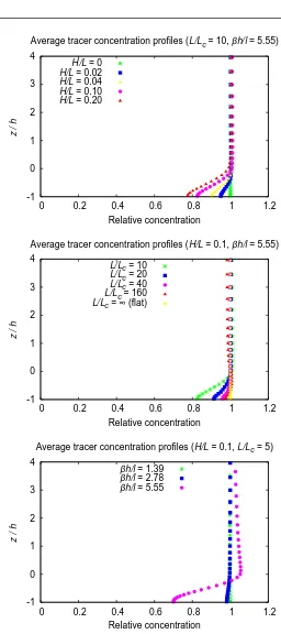
Figure 1 shows horizontally-averaged vertical profiles of relative tracer

concen-tration compared to the flat ground case for various experiments given in table 1.

In all simulations the horizontally-averaged scalar flux is the same and constant with

height since the sources and sinks of the scalar are fixed and the simulations are run to

a quasi-steady state, however there are clear differences in the horizontally-averaged

scalar concentrations. Figure 1(a) shows results for 4 simulations with different slopes

-1 0 1 2 3 4

0 0.2 0.4 0.6 0.8 1 1.2

z / h

Relative concentration

Average tracer concentration profiles (L/L_c = 10, βh/l = 5.55)

H/L _{= 0} H/L = 0.02 H/L = 0.04 H/L = 0.10 H/L _{= 0.20}

-1 0 1 2 3 4

0 0.2 0.4 0.6 0.8 1 1.2

z / h

Relative concentration

Average tracer concentration profiles (H/L = 0.1, βh/l = 5.55)

L/L_c = 10 L/L_c = 20 L/L_c = 40 L/L_c = 160 L/L_c = ∞ (flat)

-1 0 1 2 3 4

0 0.2 0.4 0.6 0.8 1 1.2

z / h

Relative concentration

Average tracer concentration profiles (H/L = 0.1, L/L_c = 5)

βh/l = 1.39 βh/l = 2.78 βh/l = 5.55

Fig. 1 Horizontally-averaged vertical profiles of tracer concentration relative to the equivalent profile over

flat ground. Height is non-dimensionalised on the canopy height,h. Canopy top is atz/h=0. The top

figure shows profiles for a fixed canopy and hill width, but for different hill heights, i.e. increasing slope,

H/l. The middle figure shows profiles for a fixed slope and canopy, but for different scale hills. The bottom

Table 1 Hill and canopy parameters for the various two-dimensional mixing length closure simulations

performed.

Parameter Values

L 100−1600 m

a 0.2−0.6 m−1

h 5−20 m

H/L 0.00625 - 0.2

L/Lc 3.75 - 240

βh/l 1.39 - 8.33

corresponds to the small hill width case described in Ross and Vosper (2005) where

vertical advection at canopy top is important. Increasing the slope leads to greater

ver-tical velocities into and out of the canopy and so increases the tracer transport by the

mean flow. This gives significantly lower average concentrations of tracer within the

canopy compared to the flat ground case, and slightly higher concentrations above.

Figure 1(b) shows profiles for 5 simulations with fixedH/L=0.1 andβh/l=5.55

and varyingL/Lc, i.e. fixed slope and canopy parameters and varying hill width. Here

decreasingL/Lc (i.e. smaller hill widths compared to the canopy adjustment scale

Lc) again leads to an increase in vertical advection at canopy top, increased tracer

transport and lower averaged concentrations within the canopy. Finally figure 1(c)

shows profiles for 3 simulations with fixedH/L=0.1,L/Lc=5 and varyingβh/l,

i.e. fixed slope, hill width and canopy density and varying canopy height. Increasing

the canopy height leads to a deeper region of flow convergence / divergence in the

increases tracer transport and leads to a significant reduction in tracer concentration

within the canopy and a slight increase above. Note that only the simulation with

the deepest canopy demonstrates a strong increase in tracer concentration above the

canopy. In all other cases the additional tracer from within the canopy is redistributed

over a sufficient depth in the boundary layer that the increases in concentration are

not large. For theβh/l=1.39 case the canopy is sufficiently shallow that no flow

sep-aration occurs. These cases withL/Lc=5 are an extreme example. For wider hills

with larger values ofL/Lc(not shown) the relative changes in average concentration

are smaller, but a broadly similar effect is seen. Deep in the canopy the average tracer

concentrations are reduced as a result of the induced flow. This is more pronounced

for deeper canopies where the induced flow is larger. In the upper canopy the change

in tracer concentration is less for most simulations. For the deepest canopies however

an increase in average concentration is observed as in the smallL/Lccase.

Overall these simulations demonstrate reductions in mean scalar concentration

deep within the canopy (for a canopy source of tracer) resulting from more efficient

transport between the canopy and the boundary layer above for steep and / or

nar-rower hills and for deeper / denser canopies. For the cases with the deepest canopy

there can actually be an increase in mean scalar concentration near canopy top. These

features can be attributed to an increase in the average vertical transport by the mean

flow between the canopy and the boundary layer above and is entirely in according

with expectations based on the analytical work of Finnigan and Belcher (2004) and

the canopy (as is the case for CO2) then the signs of the changes would be expected

to be reversed so higher concentrations would be observed deep within the canopy.

Figures 2(a) and (b) shows colour contour plots of the scalar concentration for

2 simulations - a small (L/Lc=10) and large (L/Lc=160) hill, both with slope

H/L=0.1 andβh/l=5.55. Also plotted in (c) for comparison are the results over

flat ground. The figures are plotted in a terrain following coordinate system so that

the vertical axis is height above the surface. This allows direct comparison of the

two figures, despite the differences in scale of the two hills. The figures also show

the streamlines of the flow. In both cases the streamlines entering and leaving the

canopy indicate significant vertical advection at canopy top (z/h=0). Note that the

spacing of the streamfunction contours is different within (solid lines) and above

(dotted lines) the canopy. This reflects the fact that velocities within the canopy are

much smaller than those above. The canopy-averaged results in figure 1 show that the

mean concentration in the canopy is reduced in both cases compared to the simulation

over flat ground, particularly for the small hill case. Figure 2 shows that this mean

value disguises the significant horizontal variations in scalar concentration that occur

throughout the canopy.

In both cases concentrations deep in the canopy over the upwind slope are

de-creased as a result of advection of lower concentration air from above the canopy

being transported down into the canopy and the high concentration air within the

canopy being transported up out of the canopy both through advection and enhanced

turbulent mixing. In general the concentrations in the recirculation region over the lee

-2 -1 0 1 2 -1 0 1 2 0.00 2.00 4.00 6.00 8.00 10.0 12.0 14.0 16.0 18.0 20.0 Tracer concentration

x / L

z / h

-2 -1 0 1 2

-1 0 1 2 0.00 2.00 4.00 6.00 8.00 10.0 12.0 14.0 16.0 18.0 20.0 Tracer concentration

x / L

z / h

-2 -1 0 1 2

-1 0 1 2 0.00 2.00 4.00 6.00 8.00 10.0 12.0 14.0 16.0 18.0 20.0 Tracer concentration

x / L

z / h

Fig. 2 Scalar concentration (colours) and streamlines (lines) over (a) a small hill (L=100 m), (b) a large

hill (L=1600 m) and (c) flat ground. In both (a) and (b) the hill slope is the same (H/L=0.1) and the

canopy is the same (Lc=10 m−1andβh/l=5.55). The scalars are plotted in a terrain following coordinate

system. Streamlines are plotted as lines of constant streamfunction with the solid contours at intervals of

0.2 m2_s−1_{(mostly within the canopy) and the dotted contours at intervals of 5 m}2_s−1_{(mostly above the}

location and magnitude of the maximum concentration varies between the two

simu-lations. For the small hill (a) there is a tall thin band near the separation point at the

front of the recirculation region with very high concentrations. The high

concentra-tion is associated with the stagnaconcentra-tion of the flow near the separaconcentra-tion point. Although

the mean concentration in the canopy is lower than the case over flat terrain, the

maximum concentration near the stagnation point is higher than values in the canopy

over flat terrain. In contrast, over the large hill (b) the maximum concentration is a

much wider and shallow region located at the back of the recirculation region near

the reattachment point. For intermediate hill widths (not shown) there are maxima in

concentration at both locations, with both maxima slightly weaker.

Deep in the canopy velocities and turbulent transport are small in the background

state, and the low mean velocity fields mean that there is little advection. Any induced

background flow will therefore have a significant impact on tracer concentrations

through a combination of advection and changes in turbulent transport. The

separa-tion and reattachment points are both stagnasepara-tion points of the flow and these regions

are therefore associated with low flow velocities and with reduced eddy viscosities

(and hence lower turbulent transport). This would tend to suggest that concentrations

would be highest in these regions, as observed. Whether or not the maximum is at

the separation or reattachment point seems to be rather sensitive to the details of the

flow and the turbulence scheme. Analysis of a number of simulations shows that the

minima in eddy viscosity at these two stagnation points are always quite similar in

of this eddy viscosity. In many cases the concentrations actually increase at the other

stagnation point.

A more quantitative analysis of this across all the simulations supports this broad

picture. Scaling analysis using the solution of Finnigan and Belcher (2004) gives the

ratio of vertical advection to the pressure gradient term in the upper canopy as

λ=π

4 Lc

L exp

µ

βh l

¶

(14)

(equation 36 in Finnigan and Belcher, 2004). The relationship between the location of

the maximum scalar concentration in the canopy and the role of vertical advection can

be quantified through the non-dimensional parameter which is required to be small

in order that the vertical velocity at canopy top is negligible in the analytical model

(Finnigan and Belcher, 2004; Ross and Vosper, 2005). Figure 2 suggests that the

maximum tracer concentrations are closely linked with the separation region in the

lee of the hill crest. To explore this figure 3(a) shows the location of the maximum

tracer concentration relative to the separation point, ξ= (x−xs)(xr−xs), plotted

againstλ. Herexs is the separation point andxr the reattachment point so a value

of 0 for ξ means the maximum occurs at the separation point, while a value of 1

denotes the reattachment point. The figure clearly delineates two regimes. For cases

whereλ>5 the maximum surface concentration occurs very close to the separation

point. For simulations whereλ¿5 then the maximum concentration occurs near

(but usually just upwind of) the reattachment point. In these cases the separation

region is sufficiently weak that the maximum in scalar concentration occurs near

the bottom of the hill or at the trailing attachment point of the separation region

determining the location of flow separation. For a given canopy and hill widthλis

fixed (e.g. simulations withλ∼20). Varying the hill height (and hence slope) still has

an impact on the location of the flow separation, and hence the maximum in scalar

concentration (as shown, for example, in Ross and Vosper, 2005). Increasing the hill

slope tends to shift the separation point closer to the hill summit as the stronger

adverse pressure gradient promotes earlier flow separation. In each case the scalar

maximum is very close to the separation point as shown in figure 3(a). For very sparse

canopies increasing the hill height can control whether or not separation occurs. This

is seen in the simulations withβh/l=1.39 here. Only the one with the steepest slope

exhibits separation.

The effect of the advection on the maximum concentration of the tracer is shown

in figure 3(b) which plots the maximum surface concentration normalised on the

value in the equivalent flat canopy simulation (cmax/cf lat) plotted againstλ. Although

the data does not collapse as well as figure 3(a) it is clear that for small values ofλ

where advection is small then (as expected)cmax/cf lat∼1 and concentrations vary

little from those over a flat canopy. In contrast, forλ>5 there is a larger spread in

the values ofcmax/cf lat. Maximum concentrations are increased - in this case by up

to 50% in some simulations, although again the actual maximum value is not solely

determined byλ. For a fixed canopy and hill width, then increasing the hill height (and

hence the slope,H/L) leads to an increase in the maximum tracer concentration as a

result of more pronounced differences in the eddy viscosity between the separation

0 0.2 0.4 0.6 0.8 1

0 5 10 15 20 25 30 35 40 45

(

x-x

s

)/(

xr

-x

s

)

λ

βh/l = 8.33

βh/l = 5.55

βh/l = 4.17

βh/l = 2.78

βh/l _{= 1.39}

0 0.5 1 1.5 2

0 5 10 15 20 25 30 35 40 45

cmax

/ c

flat

λ

βh/l = 8.33

βh/l = 5.55

βh/l = 4.17

βh/l _{= 2.78} βh/l = 1.39

Fig. 3 (a) The non-dimension location of the scalar maximum relative to the separation regionξ=

(xtrmax−xs)/(xr−xs)wherextrmaxis the location of the maximum surface tracer concentration,xsis the

location of the separation point andxris the reattachment point plotted against vertical velocity parameter,

λfor different non-dimensional canopy depthsβh/l. (b) The maximum tracer concentration normalised

A number of simulations were conducted with twice the horizontal and vertical

resolutions to check the sensitivity of the results to model resolution. Doubling the

resolution made no qualitative difference to the results. From a quantitative point

of view there was almost no difference in the location of the separation region, or

the maximum tracer concentrations deep in the canopy, although there was a slight

increase in the calculated depth of the separation region with increased vertical

res-olution. Most sensitivity was observed at canopy top, where the strong vertical shear

in the wind makes a high vertical resolution most necessary. Even here differences in

canopy-top velocities and tracer concentrations were at most a few percent.

The conclusion of this analysis is that maximum concentrations almost always

oc-cur close to stagnation points. In the one-and-a-half order closer model the details of

which separation point exhibits the highest concentration appears to be linked to the

scale of the hill and the importance of vertical advection at canopy top. Smaller scale

hills, where vertical advection is significant at canopy top, tend to exhibit minima of

turbulent kinetic energy and eddy viscosity and maxima of tracer concentration at the

separation point near the summit. Larger scale hills where canopy top vertical

advec-tion is smaller show the minima of turbulent kinetic energy and eddy viscosity and

the maxima of tracer concentration at the reattachment point near the foot of the hill.

The details of which separation point exhibits the maximum tracer concentration

are sensitive to small differences in the induced flow which lead to small differences

in the turbulent kinetic energy and calculated eddy viscosity. The concentrations are

perhaps not surprising, but does mean that conclusions on the tracer concentrations

in the deep canopy should be treated with some caution.

There are only a couple of simulations where the canopy is so shallow and sparse

that no separation occurs at all. In these cases the maximum concentrations are

ob-served near the foot of the hill similar to that obob-served in figure 2(b). At this location

the adverse pressure gradient over the lee slope generates the lowest wind speeds and

hence the eddy viscosity is smallest.

Above the canopy both the simulations in figure 2 exhibit horizontal variations

in concentration. The scalar concentration isolines do not exactly coincide with the

streamlines, suggesting that although advection plays an important role in

modify-ing the scalar concentrations over the hill, turbulent fluxes are also important. The

horizontal variations are larger over the small hill, as expected, since the vertical

ve-locities are larger. These general features are also reproduced in the other simulations

(not shown). The analysis of section 3 gives a scaling for canopy top perturbations

in tracer concentration. Here the magnitude of the canopy top perturbations is

char-acterised by the standard deviation of the canopy top scalar concentration. Figure 4

shows the standard deviation of the canopy top scalar concentration plotted against

the scaling for the canopy top tracer perturbation,c. Results are plotted only for

simu-lations withH/L<0.1 andL/Lc≥50. This excludes the narrowest hills and steepest

slopes where the Finnigan and Belcher (2004) model, and hence the tracer scaling, is

not valid. Despite the fact that the analysis excludes the contribution to the variability

from the deep canopy, the scaling does a good job in collapsing the data from a wide

0 0.01 0.02 0.03 0.04 0.05 0.06 0.07 0.08 0.09 0.1 0.11

0 0.0005 0.001 0.0015 0.002 0.0025 0.003 0.0035

σc

(H / L_{) (}L_c / L_{) (}U_{0 /} U_h)2 Sh / U_h Tracer variability at canopy top

βh/l = 8.33

βh/l = 5.56

βh/l = 5.56

βh/l = 4.17

βh/l = 2.78

βh/l = 1.39

Fig. 4 The standard deviation of the tracer concentration at canopy top plotted against the scaling for

tracer concentration from equation (12). Only experiments withH/L<0.1 andL/Lc≥50 are included.

variations in tracer concentrations may not be overly sensitive to the deep canopy

so-lution, and hence may well be successfully predicted by a mixing length turbulence

closure scheme, unlike the deep canopy concentrations. For the narrower and steeper

hills then vertical advection in the upper canopy plays an increasingly important role

and the scaling appears no longer to hold (results not shown), with advection and the

concentrations deeper in the canopy playing a bigger role.

Figure 5 shows the canopy top advection term for a number of different

simu-lations. In Figure 5(a) the advection is non-dimensionalised on the source term and

results are shown for a fixed canopy (βh/l=5.56,Lc=10 m) and slope (H/L=0.02)

and only the scale of the hill is changed. For the widest hills advection is small

com-pared to the source term, while for the narrowest hill (L=100 m) the advection term

and so advection plays an important role, as might be expected. The other interesting

feature is that advection is particularly important over the lee slope in the

recircu-lation region which may be important for interpreting flux measurements over real

forests. Figure 5(b) shows the advection over a range of different canopies and slopes

for the widest hills (L=1600 m). In this case advection is small compared to the

source term and the scaling from (13) is expected to be valid. Results are shown

non-dimensionalised on this scaling. The scaling is reasonably successful in collapsing

the results over the range of canopies and slopes. For a fixed canopy but different

slopes the collapse is excellent (βh/l=5.56 and Lc=10 m withH/L=0.02 or

H/L=0.00625). For different canopies the scaling broadly predicts the magnitude

of the advection terms, but there are some in magnitude and in the phase which reflect

the fact that the scaling ignores the contribution to the advection from flow deep in

the canopy. Nonetheless the scaling is a useful means of predicting the importance

of scalar advection in these wide hill cases where advection is relatively weak. The

scaling is less successful in the narrow hill regime where advection becomes large

(not shown).

These simulations using the one-and-a-half order turbulence closure scheme and a

fixed source of tracer within the canopy all demonstrate that advection can be

impor-tant in modifying tracer concentrations over canopy-covered hills. In particular,

wher-ever there is significant vertical advection at canopy top (small hills / dense canopies

/ deep canopies) transport is enhanced. This transport leads to lower mean

concentra-tions within the canopy and significant horizontal variaconcentra-tions in tracer concentration.

-1 -0.5 0 0.5 1

-2 -1.5 -1 -0.5 0 0.5 1 1.5 2

Advection term / source term

x / L

Non-dimensional advection term at canopy top

L=100m

L=200m

L=400m

L=800m

L=1600m

-400 -300 -200 -100 0 100 200 300 400

-2 -1.5 -1 -0.5 0 0.5 1 1.5 2

Advection term / advection scaling

x / L

Non-dimensional advection term at canopy top

H/L=0.02, βh/l=5.56, L_c=10m

H/L=0.02, βh/l=8.33, Lc=6.7m

H/L=0.02, βh/l=5.56, L_c=20m

H/L=0.02, βh/l=2.78, L_c=20m

H/L_=6.25E-3, βh/l_=5.56, L_c=10m

Fig. 5 Plots of the canopy top advection term as a function of non-dimensional distance across the hill

for a number of different simulations. In (a) the slope and canopy are fixed (H/L=0.02,βh/l=5.56 and

only the scale of the hill is changed (L=100−1600 m. In (a) the advection term is scaled on the source

term,S. In (b) a number of different simulations with fixed widthL=1600 m, but varying canopy and

horizontal variations are closely linked to flow separation and recirculation within

the canopy and therefore scaling parameters which quantify these dynamic effects

are also useful in explaining different regimes of behaviour in tracer concentrations.

A simple scaling argument based on the analytical solution for flow over a forested

hill successfully collapses the observed tracer perturbations and also the tracer

ad-vection terms at canopy top over a wide range of simulations.

5 Large-eddy simulations

5.1 Large eddy simulations over a small hill

Simulations with the one-and-a-half order closure scheme are useful because the

scheme is simple and therefore the simulations are quick to run. This allows a wide

range of parameter space to be investigated. Given the uncertainties over mixing

length closure schemes, and in particularly the sensitivity of tracer concentrations

deep in the canopy to the turbulence scheme, then some form of validation of the

results is however desirable. One way to address this is through the use of large eddy

simulations. Such simulations are significantly more computationally expensive and

therefore a limited number of simulations are possible, however they can help to

vali-date conclusions drawn from the simpler one-and-a-half order closure scheme results.

Large eddy simulations of flow over both a flat surface and a small hill (H=10 m,

L=100 m) are presented. The model setup is described in section 2.1 and is

iden-tical to that used in Ross (2008) with the addition of a passive tracer. Ross (2008)

-1 -0.5 0 0.5 1

-2 -1.5 -1 -0.5 0 0.5 1 1.5 2

-400 -300 -200 -100 0 100 200 300 400

z / h

x / L Tracer (arbitrary units)

LES LES (flat)

β = 0.3

β = 0.35

Fig. 6 Profiles of tracer (in arbitrary units) across a small hill from a LES simulation (solid black line),

from a simulation using the one-and-a-half order closure scheme (red dashed line -β=0.3 and blue

dot-dashed line -β=0.35). Also shown for comparison are the results from the LES over flat ground (green

dotted line).

were different between LES and mixing-length simulations, the mean flow and broad

dynamic features were in good agreement. This is primarily because the flow is

dom-inated by turbulence generated in the shear layer at canopy top and this is well

repre-sented in the mixing-length scheme.

Figure 6 shows profiles of the scalar concentration across the hill. Results from

the large-eddy simulations over the hill (solid black line) are compared with results

from simulations using the one-and-a-half order closure scheme over the same hill

and from the LES model over flat ground. The canopy, hill and flow parameters are

one-and-a-half order results are presented for two different values of the empirical parameter

β. The valueβ=0.30 corresponds to the value assumed in Finnigan and Belcher

(2004) and Ross and Vosper (2005), while the valueβ=0.35 was shown by Ross

(2008) to better match the large-eddy simulation results in terms of the surface

pres-sure field and wind speed and shear stress profiles. Here we see that all three

simula-tions over the hill give very similar results in terms of scalar concentration profiles,

suggesting that the scalar transport is not too sensitive to details of the turbulence

scheme in this case. The results show small, but significant, differences from the

re-sults over flat ground. These differences are most noticeable over the upwind slope

where mean-flow transport leads to lower concentrations deep in the canopy over the

upwind slope compared to the flat case. Over the lee slope the concentrations in the

recirculation region are slightly increased compared to the flat case, but the

differ-ences are smaller than over the upwind slope. Differdiffer-ences in the tracer profiles over

the hill appear principally in the separation region over the lee slope. Again the value

ofβ=0.35 better reproduces the LES results, particularly near canopy top over the

lee slope. Note that both values of βlie within the range of observed values from

real forest canopies. These results are qualitatively similar to those observed using

the one-and-a-half order closure scheme in section 2. A closer examination of the

tracer concentrations shows that the region of high tracer concentration over the lee

slope has a lower maximum and is more spread out in the LES simulation compared

to the mixing length closure scheme. This is entirely consistent with figure 5(b) of

Ross (2008) which showed that the LES predicted higher values for the turbulent

mixing. This probably reflects the fact that although there is little mean flow in the

deep canopy there is significant variability in the flow and in the tracer concentrations

resulting from the flow in the upper canopy and above penetrating down.

5.2 The turbulent Schmidt number

The first-order mixing length closure scheme assumes that the Reynolds shear stress,

τi j=−ρu0iu0j, and Reynolds-averaged turbulent tracer mixing term,u0ic0are given by

u0

iu0j =Km

µ

∂ui

∂xj+

∂uj

∂xi

¶

(15a)

u0

ic0 =Kc_∂∂_xc

i. (15b)

In the first order turbulence schemeKmis determined using a mixing length closure.

Ross (2008) examined the validity of this mixing length approximation forKmusing

the LES results. Implicit in the first order mixing length closure is the assumption that

the turbulent Schmidt number (the ratio of the turbulent diffusivities for momentum

and scalar),

Sc≡Km

Kc (16)

is equal to 1, i.e. momentum and scalars are mixed by turbulence in exactly the same

way. Experimental observations in the atmospheric boundary layer do not necessarily

satisfy equation 15b for all components,i. In generalKmandKcare defined to ensure

that this is a reasonable approximation in the direction of the dominant turbulent flux.

To calculateKmandKcfrom the LES data the vertical components are taken so

Km= u

0_w0

∂u/∂z+∂w/∂x (17a)

Kc= w

0_c0

In the boundary layer the Schmidt number is generally close to 1, however

obser-vations in forest canopies show that the Schmidt number decreases to about 0.5 in

the reduced surface layer (RSL) which extends up to a few canopy heights above

canopy top (Harman and Finnigan, 2008). This is also observed in the LES

simula-tions over flat terrain (see figure 7). Within the canopy the LES then demonstrates a

sharp increase in the Schmidt number up to a maximum of about 2 at a height of 5m

above the ground, before it then decreases again towards the surface. Variations in the

Schmidt number within the canopy are perhaps unsurprising as mixing-length closure

schemes are known not to perform particularly well there (see e.g. Ross, 2008). From

a dynamical point of view this has a relatively small impact since turbulent

momen-tum fluxes are small deep within the canopy due to the small vertical wind shear.

This is not necessarily the case for tracer fluxes, where there may still be significant

gradients in tracer concentration.

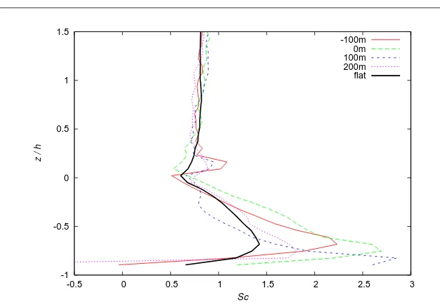
Figure 7 also shows profiles of the Schmidt number derived from the large-eddy

simulation at four different locations across the hill. These are slightly more noisy

as averaging is only done in the lateral direction and over time on the hill, whereas

streamwise averaging is also performed for the simulation over flat ground. All four

profiles show similar trends to the results over flat ground with the Schmidt number

decreasing from around 1 well above the canopy to a minimum near canopy top, and

then increasing within the canopy to a maximum at about 5m above the ground. There

are however significant quantitative differences between profiles.

Well above the forest canopy results are similar for all profiles. Closer

-1 -0.5 0 0.5 1 1.5

-0.5 0 0.5 1 1.5 2 2.5 3

z / h

Sc -100m 0m 100m 200m flat

Fig. 7 Profiles of the turbulent Schmidt number on flat ground and at 4 locations over the hill derived from

the large-eddy simulations. Canopy top is atz/h=0.

-1 -0.5 0 0.5 1 1.5

-0.2 0 0.2 0.4 0.6 0.8 1 1.2 1.4

z / h

Km -100m 0m 100m 200m flat -1 -0.5 0 0.5 1 1.5

-0.2 0 0.2 0.4 0.6 0.8 1 1.2 1.4

z / h

Kc -100m 0m 100m 200m flat

Fig. 8 Profiles of the turbulent diffusivity for (a) momentum,Kmand (b) tracer,Kcon flat ground and at 4

locations over the hill derived from the large-eddy simulations. Canopy top is atz/h=0.

over the hill, but by similar amounts. This is due to increases in both the horizontally

averaged momentum and scalar fluxes. This is perhaps slightly surprising and may

be due in part to starting the LES averaging before the simulation has settled to a

calculated values ofScabove the canopy vary little over the hill and compare very

well with the results over flat ground. The values ofKmandKcincrease particularly

above the recirculation region (x=200 m) in what is likely to be a real dynamic effect

due to the hill. Just above canopy top the systematic variations betweenKm andKc

compared to the flat case are smaller but there are much more significant differences

in the Schmidt number with lower values than over flat ground at the summit of the

hill and larger values elsewhere over the hill. The larger values of the Schmidt

num-ber in this region, up to values of about 1, are principally due to enhanced values of

Kmin this region compared to over flat ground. This suggests that increased shear and

vertical advection at canopy top are important in modifying turbulent transport just

above the canopy, which is entirely in accord with the scaling analysis of section 3.

Within the canopy the Schmidt numbers over the hill exceed those over flat

ground in most locations, and in particular the maximum values at low level are

sig-nificantly larger, up to about 3. This is due to a combination of increased values ofKm

over the lee slope (100m) and in the valley (200m) , and reduced values ofKcon the

upwind slope (-100m) and near the summit (0m). The only place within the canopy

where the Schmidt number is less over the hill than on flat ground is in the upper part

of the canopy over the lee slope (100m). This is in the recirculation region, and the

low wind shear in this region leads to reduced values ofKmcompared to other parts

of the canopy, although the impact onKcis less.

What these large-eddy simulation results show is that the relationship between

KmandKcis not simple within and above forest canopies. This particular small hill,

variability in the Schmidt number potentially makes modelling of tracer transport

us-ing mixus-ing length closure schemes difficult. It would be possible to devise a scheme

whereScscaled with height to match results over flat ground, as done in Harman and

Finnigan (2008), however these results suggest that even this approach might not be

sufficient over hills. Having said all this it is then perhaps surprising that the tracer

profiles from the one-and-a-half order model agree so well with those from the LES

in figure 1. Perhaps this suggests that tracer advection is actually dominating in these

cases and so errors in turbulent tracer fluxes are less important. This does seem to

agree with the conclusions of the scaling analysis in section 3 that the leading order

perturbation in the turbulent fluxes is zero. This is clearly a topic for further research

in terms of modelling scalar transport within and above forest canopies over complex

terrain. In particular it would be interesting to run large eddy simulations for much

wider hills where advection is smaller and hence turbulent transport is more

impor-tant, however computational requirements preclude this with the current version of

the model described here.

6 Implications for flux measurements

Observations of carbon uptake by forests are frequently made using eddy-covariance

flux measurements on a large tower (e.g. the FLUXNET project Baldocchi et al.,

2001) and assuming that this is representative of a forest. Many forested sites are not

truly flat though and so the assumptions of horizontal homogeneity are not exactly

met. The potential impact of advection on the flux measurements has to be

errors in flux measurements (e.g. Wilson et al., 2002; Belcher et al., 2008),

how-ever this work shows that even under neutral, strong wind conditions advection may

be non-negligible. There is evidence of this from the FLUXNET sites. The study of

Wilson et al. (2002) demonstrated an average imbalance of around 20% in the energy

balance, even in daytime conditions. The imbalance was observed even for

well-mixed conditions (i.e. more neutral flow with stronger winds), although it increased

for lower wind speeds and was much larger in nocturnal conditions. The advective

effects demonstrated by this work, even for large hills with relatively small slopes, are

certainly consistent with these observations. Figure 9 shows the turbulent scalar flux

(non-dimensionalised on the depth integrated scalar source term) at canopy top and

heighthabove the canopy for three different hills with the same slope (H/L=0.1),

but different scales (L=100,200,400,1600). In each case the canopy and the

uni-form scalar source term are the same (βh/l=5.55,Lc=10 m,S=10−2m−3s−1).

For steady-state flow over flat ground the non-dimensional scalar flux is one since

production in the canopy is balanced by turbulent transport at canopy top. For the

widest hill, with relatively weak canopy-top vertical velocities the canopy-top scalar

fluxes only vary a small amount across the hill. Note that the total flux integrated

across the hill is slightly less than the flat ground case, suggesting that advection is

responsible for a small net transport of scalar out of the canopy. As the scale of the

hill decreases the variability in the canopy-top fluxes increases significantly. At some

points over the smallest hill point measurements of the canopy top turbulent flux vary

by up to a factor of three compared to the source term. Variations at a heighthabove

0 0.5 1 1.5 2 2.5 3

-2 -1.5 -1 -0.5 0 0.5 1 1.5 2

Turbulent flux / depth integrated source

x / L

Canopy top tracer vertical turbulent flux

L = 100m

L = 200m

L = 400m

L = 1600m flat 0 0.5 1 1.5 2 2.5 3

-2 -1.5 -1 -0.5 0 0.5 1 1.5 2

Turbulent flux / depth integrated source

x / L

Tracer vertical turbulent flux at height h above canopy

L = 100m

L = 200m

L = 400m

L = 1600m flat

Fig. 9 Canopy-top turbulent scalar flux (normalised on the depth-integrated canopy source term) plotted

against the position across the hill (non-dimensionalised on the hill width) for different hills (simulations

3, 5 and 7 in §2).

top. The increased height above the canopy smooths out some of the canopy-induced

variability. For the smallest hill there is still a difference of up to a factor of two

compared to the flat-ground case.

A further consideration when interpreting flux measurements is that the flow into

and out of the canopy means that streamlines are not parallel to the terrain or to

canopy top, and therefore techniques which rotate sonic anemometer measurements

into a mean flow coordinate system or use a planar fit to the flow data as a coordinate

system (see e.g. Lee et al., 2004) may not give the expected results. In particular,

the lack of symmetry to a reversal of wind direction means that even for an ideal

symmetrical hill and ideal conditions the averaged wind data will not lie in a plane.

For large-scale hills the effect will be relatively small, but for smaller scale hills it

could be significant.

Modelling studies such as these are not yet practical for correcting or scaling

important indications of the type and magnitude of errors that may be introduced

through neglecting such effects. They may also provide guidance into the most

suit-able locations for making flux measurements which are truly representative of a larger

area.

7 Conclusion

This paper provides a systematic investigation of the impact of hills on scalar

concen-tration and transport within and above a forest canopy. With a fixed uniform source

of scalar within the canopy the dynamics of the canopy - boundary layer interactions

(previously studied by e.g Finnigan and Belcher, 2004; Ross and Vosper, 2005)

dom-inate. Over hills the pressure field resulting from the presence of the hill drives flow

into and out of the canopy and this dynamical process acts like a pump to remove

scalars more efficiently from the canopy space. This reduces the mean

concentra-tion of scalar within the canopy for a fixed source term. This effect is particularly

strong for small-scale hills where the canopy-atmosphere mean flow is largest.

Al-though the overall effect is to reduce mean scalar concentrations in the canopy, there

is a large spatial variability in concentrations in the canopy, with the maximum

con-centrations at a given canopy depth often exceeding those over flat ground. This is

closely linked to flow separation in the lee of the hill trapping scalars in the canopy. In

cases where there is moderately strong vertical advection at canopy top then the

max-imum concentrations occur near the separation point. Low wind speeds and shear in

this region result in weak turbulent transport and long canopy residence times for the

are relatively robust it is likely that the details of tracer concentrations in the canopy

will be sensitive to the turbulence closure scheme. Canopy top tracer variations can

be successfully predicted using a simple scaling argument which neglects the deep

canopy. This works well for relatively wide hills and suggests that in these cases first

order closure schemes may be more successful than anticipated in predicting tracer

concentrations. Similar results for time-averaged scalar concentrations are seen for

a large-eddy simulation of flow over a small hill based on the simulations in Ross

(2008). The LES does highlight the unsteady and intermittent nature of the flow in

the canopy. Calculations of the Schmidt number in the LES also suggest that the

com-mon assumption that momentum and scalars are transported in the same way is not

valid within and just above the canopies, with significant variations in the Schmidt

number in the vertical and across the hill. In principle at least some of this variability

could be represented with a parametrisation of the Schmidt number in the canopy,

but whether this is the most significant source of uncertainty in mixing length closure

models for canopy flows remains to be studied.

Acknowledgements This work was partially supported by the UK Natural Environment Research

Coun-cil (NERC) through grant NE/C003691/1. The author would like to thank the anonymous reviewers who’s

thorough comments significantly improved this paper.

References

Baldocchi D, Falge E, Gu LH, Olson R, Hollinger D, Running S, Anthoni P,

Bern-hofer C, Davis K, Evans R, Fuentes J, Goldstein A, Katul G, Law B, Lee XH,

Valentini R, Verma S, Vesala T, Wilson K, Wofsy S (2001) FLUXNET: A new

tool to study the temporal and spatial variability of ecosystem-scale carbon

diox-ide, water vapor, and energy flux densities. Bull Amer Met Soc 82:2415–2434

Belcher SE, Finnigan JJ, Harman IN (2008) Flows through forest canopies in

com-plex terrain. Ecol Apps 18:1436–1453

Brown AR, Hobson JM, Wood N (2001) Large-eddy simulation of neutral turbulent

flow over rough sinusoidal ridges. Boundary-Layer Meteorol 98:411–441

Dupont S, Brunet Y, Finnigan JJ (2008) Large-eddy simulation of turbulent flow over

a forested hill: Validation and coherent structure identification. Quart J Roy

Mete-orol Soc 134:1911–1929

Feigenwinter C, Bernhofer C, Eichelmann U, Heinesch B, Hertel M, Janous D, Kolle

O, Lagergren F, Lindroth A, Minerbi S, Moderow U, M¨older M, Montagnani L,

Queck R, Rebmann C, Vestin P, Yernaux M, Zeri M, Ziegler W, Aubinet M (2008)

Comparison of horizontal and vertical advective CO2 fluxes at three forest sites.

Agric For Meteorol 148(1):12–24

Finnigan JJ (2000) Turbulence in plant canopies. Annu Rev Fluid Mech 32:519–571

Finnigan JJ (2008) An introduction to flux measurements in difficult conditions. Ecol

Apps 18(6):1340–1350

Finnigan JJ, Belcher SE (2004) Flow over a hill covered with a plant canopy. Quart J

Roy Meteorol Soc 130:1–29

Finnigan JJ, Brunet Y (1995) Turbulent airflow in forests on flat and hilly terrain. In:

Harman IN, Finnigan JJ (2008) Scalar concentration profiles in the canopy and

rough-ness sublayer. Boundary-Layer Meteorol 129(3):323–351

Hunt JCR, Leibovich S, Richards KJ (1988) Turbulent shear flow over low hills.

Quart J Roy Meteorol Soc 114:1435–1470

Katul GG, Mahrt L, Poggi D, Sanz C (2004) One- and two-equation models for

canopy turbulence. Boundary-Layer Meteorol 113:81–109

Katul GG, Finnigan JJ, Poggi D, Leuning R, Belcher SE (2006) The influence of hilly

terrain on canopy-atmosphere carbon dioxide exchange. Boundary-Layer Meteorol

118:189–216

Lee X, Massman W, Law B (eds) (2004) A handbook of micrometeorology: A guide

for surface flux measurements. Kluwer academic publishers

Patton EG, Katul GG (2009) Turbulent pressure and velocity perturbations induced

by gentle hills covered with sparse and dense canopies. Boundary-Layer Meteorol

133:189–217

Pinard JDJP, Wilson JD (2001) First- and second-order closure models for wind in a

plant canopy. J Appl Meteor 40(10):1762–1768

Poggi D, Katul GG (2007a) The ejection-sweep cycle over bare and forested gentle

hills: a laboratory experiment. Boundary-Layer Meteorol 122:493–515

Poggi D, Katul GG (2007b) An experimental investigation of the mean momentum

budget inside dense canopies on narrow gentle hilly terrain. Agric For Meteorol

144:1–13

Poggi D, Katul GG (2007c) Turbulent flows on forested hilly terrain: the recirculation

Ross AN (2008) Large eddy simulations of flow over forested ridges.

Boundary-Layer Meteorol 128:59–76

Ross AN, Vosper SB (2005) Neutral turbulent flow over forested hills. Quart J Roy

Meteorol Soc 131:1841–1862

Wilson K, Goldstein A, Falge E, Aubinet M, Baldocchi D, Berigier P, Bernhofer C,

Ceulmans R, Dolman H, Field C, Grelle A, Ibrom A, Law BE, Kowalski A, Meyers

T, Moncrieff J, Monson R, Oechel W, Tenhunen J, Valentini R, Verma S (2002)

Energy balance closure at FLUXNET sites. Agric For Meteorol 113:223–243

Wood N, Mason PJ (1993) The pressure force induced by neutral, turbulent flow over

hills. Quart J Roy Meteorol Soc 119:1233–1267

Zeri M, Rebmann C, Feigenwinter C, Sedlak P (2010) Analysis of short periods

with strong and coherent CO2 advection over a forested hill. Agric For