Learning for Cross-layer Resource Allocation in the Framework of Cognitive Wireless Networks

(1)

Rochester Institute of Technology

RIT Scholar Works

Theses Thesis/Dissertation Collections

8-2016

Learning for Cross-layer Resource Allocation in the

Framework of Cognitive Wireless Networks

Wenbo Wang

[email protected]

Follow this and additional works at:http://scholarworks.rit.edu/theses

Recommended Citation

(2)

LEARNING FOR CROSS-LAYER RESOURCE

ALLOCATION IN THE FRAMEWORK OF

COGNITIVE WIRELESS NETWORKS

by

Wenbo Wang

DISSERTATION

Presented to the Faculty of the Golisano College of Computer and Information Sciences

Rochester Institute of Technology in Partial Fulfillment

of the Requirements

for the Degree of

DOCTOR OF PHILOSOPHY

(3)

Learning for Cross-Layer Resource Allocation in the Framework of

Cognitive Wireless Networks

by

Wenbo Wang

Committee Approval:

We, the undersigned committee members, certify that we have advised and/or supervised the candidate on the work described in this dissertation. We further certify that we have reviewed the dissertation manuscript and approve it in partial fulfillment of the requirements of the degree of Doctor of Philosophy in Computing and Information Sciences.

______________________________________________________________________________

Dr. Andres Kwasinski Date

Dissertation Advisor

______________________________________________________________________________

Dr. Zhu Han Date

Dissertation Committee Member

______________________________________________________________________________

Dr. Pengcheng Shi Date

______________________________________________________________________________

Dr. Kaiqi Xiong Date

______________________________________________________________________________

Dr. Shanchieh Jay Yang Date

______________________________________________________________________________

Dr. Drew N. Maywar Date

Dissertation Defense Chair

Certified by:

______________________________________________________________________________

Dr. Pengcheng Shi Date

(4)

Acknowledgments

I would like to thank my adviser, Dr. Andres Kwasinski, for all his advice, support and patience since I entered the Ph.D. program of Golisano College of Computer and Information Sciences in RIT. I would like to thank Prof. Shanchieh Jay Yang, Prof. Zhu Han, Dr. Kaiqi Xiong and Prof. Pengcheng Shi for being on my dissertation committee. I also would like to thank Prof. Shanchieh Jay Yang and Prof. Pengcheng Shi for their invaluable advice and encouragement when I was at the lowest point of my life.

Finally, I would like to thank my parents for their unconditional love and

support. Without their support, I would not have been able to complete my

(5)

Abstract

LEARNING FOR CROSS-LAYER RESOURCE ALLOCATION IN

THE FRAMEWORK OF COGNITIVE WIRELESS NETWORKS

Author: Wenbo Wang

Supervisor: Andres Kwasinski, Ph.D. Degree: Doctor of Philosophy

Golisano College of Computing and Information Sciences, 2016

The framework of cognitive wireless networks is expected to endow wireless devices with a cognition-intelligence ability with which they can efficiently learn and respond to the dynamic wireless environment. In this dissertation, we focus on the problem of developing cognitive network control mechanisms without knowing in advance an accurate network model. We study a series of cross-layer resource allocation problems in cognitive wireless networks. Based on model-free learning, optimization and game theory, we propose a framework of self-organized, adaptive strategy learning for wireless devices to (implicitly) build the understanding of the network dynamics through trial-and-error.

(6)

In the second part of this work, we extend our study from the single-agent to a multi-agent decision-making scenario, and study the energy-efficient power allocation problems in a two-tier, underlay heterogeneous network and in a self-sustainable green network. For the heterogeneous network, we propose a stochastic learning algorithm based on repeated games to allow individual macro- or femto-users to find a Stackelberg equilibrium without flooding the network with local action information. For the self-sustainable green network, we propose a combinatorial auction mechanism that allows mobile stations to adaptively choose the optimal base station and sub-carrier group for transmis-sion only from local payoff and transmistransmis-sion strategy information.

(7)

List of Tables

2.1 Transition probabilities of the Markov model for layered video

transmission . . . 21

2.2 Main parameters used in the video streaming simulation. . . . 27

2.3 Retransmission frequencies for the learning processes in Figure 2.4. . . 27

2.4 Performance comparison between different transmission mech-anisms. . . 29

3.1 Main Parameters Used in the Femtocell Network Simulation . 54 3.2 Main Parameters Used in the Self-Learning Algorithm . . . 57

4.1 Iterative subcarrier auction mechanism . . . 76

4.2 Bisection Based Power Price Updating . . . 77

(11)

List of Figures

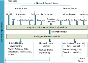
1.1 Relationship between cognition and intelligence in a cognitive wireless network. . . 3

2.1 Dependency DAG of one GoP with both temporal and quality scalability. . . 13 2.2 The state transition for video layer n of GoP i . . . 19 2.3 Layered video transmission Markov chain. . . 21 2.4 Transmission performance and policy evolution with the

pro-posed adaptive policy learning mechanism. (a) Frame PSNR v.s. frame number. (b) Source-coding rate v.s. frame number. 28

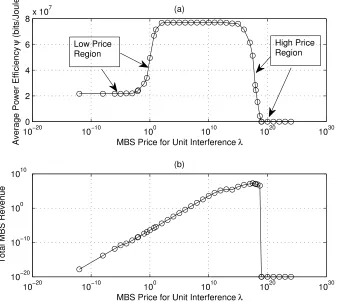
3.1 Influence of the unit interference price on the NE of the contin-uous follower-game. (a) Average power efficiency at the NE vs. the unit price λ; (b) total revenue collected by the MBS at the NE vs. the unit price λ. . . 55 3.2 MBS revenue and FU power efficiency at the SEs. (a) MBS

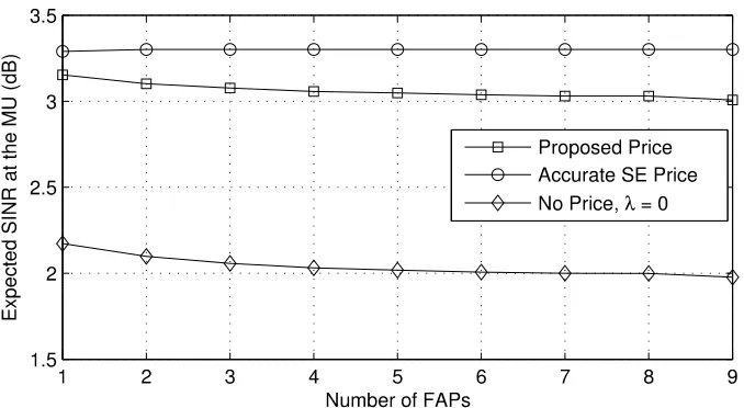
revenue vs. the number of FAPs; (b) FU power efficiency vs. the number of FAPs. . . 56 3.3 Expected equilibrium SINR at the MU vs. the number of FAPs. 57 3.4 Influence of the unit interference price on the NE of the discrete

follower-game. (a) Expected average power efficiency at the NE vs. the unit price λ; (b) total revenue collected by the MBS at the NE vs. the unit price λ. . . 58 3.5 Expected MBS revenue and FU power efficiency at the SEs in

(12)

4.1 An example of a microgrid with five BSs, in which the power source is installed as a combination of different green power generators. . . 63 4.2 The follower subgame (i.e., the subcarrier auction game)

per-formance evolution during one time slot. (a) Total effective throughput v.s. auction rounds; (b) average power consump-tion v.s. aucconsump-tion rounds. . . 78 4.3 Performance evolution with power pricing. (a) Power

consump-tion/generation v.s. time; (b) total throughput v.s. time. . . . 81 4.4 Performance comparison. (a) Expected throughput without

power pricing; (b) percentage of operational time. . . 82

5.1 Radio activities in a two-channel CRN with coordinated peri-odic sensing in the secondary network. . . 89 5.2 SU links in a CRN with two clusters. . . 92 5.3 Attacker-free sensor grid network over a single PU channel. . . 119 5.4 Strategy evolution: relay selection probability vs. iteration

number. . . 119 5.5 An attacker-free CRN over 2 PU channels. . . 120 5.6 Strategy evolution: channel-relay selection probability vs.

iter-ation number. . . 120 5.7 Average path delay vs. number of flows for different algorithms. 121 5.8 (a) Frequency of connections to malicious nodes vs. scale for

(13)

Chapter 1

Introduction and Background

1.1

Cognitive Radio Networks

The original concept of Cognitive Radio (CR) was first proposed a little over one decade ago [1]. In a broad sense, CR is defined as a prototypical software-defined radio that adopts a radio-knowledge-representation language to au-tonomously learn the dynamics of wireless environments and adapt to changes of application/protocol requirements. In recent years, Cognitive Radio Net-works (CRNs) have been widely recognized from a high-level perspective as

an intelligent wireless communication system. A device in a CRN is expected to be aware of its surrounding environment and uses the methodology of understanding-by-building to reconfigure the operational parameters in real-time to achieve optimal network performance [2,3]. In the framework of CRNs, the following abilities are typically emphasized:

• radio-environment awareness by sensing (cognition) in a time-varying radio environment;

(14)

• cost-efficient and scalable network configuration.

Many recent studies on CR technologies focus on radio-environment aware-ness in order to enhance spectrum efficiency. This leads to the concept of Dynamic Spectrum Access (DSA) networks [4], which are featured by a novel PHY-MAC architecture (namely, primary users and secondary users) for op-portunistic spectrum access based on the detection of spectrum holes [5]. It is worth noting that by emphasizing the network architecture of spectrum sharing between the licensed/primary networks and the unlicensed/secondary networks [4], “DSA networks” is frequently considered a terminology that is interchangeable with “CR networks” [3]. The rationale behind such a consid-eration is that a secondary network relies on spectrum cognition modules to make proper decisions for seamless spectrum access without interfering the pri-mary transmissions. For this category of works in the literature, “learning” is a set of techniques for feature classification of primary signal identification [6]. For an overview of the relevant techniques, the readers may refer to recent survey works in [7–9].

(15)

Network Context Space

Internal States External States

Mobility Protocols Platform Environment Other Devices Network

PHY MAC/Link Application Geography Regulation Interference

Constraints Behavior Profile Topology

Cognition (Information Collection) Module

Intelligent Decision Module

PHY/MAC/Link Layer Control

Network Layer Control

N

e

tw

or

k

E

nv

ironm

e

nt

Information Flow Feedback

Control Signals Power, Antenna, Rate,

Modulation, Multi-Access, FEC/ARQ, ...

Routing, Traffic Enginnering, ...

[image:15.612.139.494.117.374.2]

Application/Transport Layer Control Source Coding, QoS, Security, Handoff, ...

Figure 1.1: Relationship between cognition and intelligence in a cognitive wireless network.

(16)

Designing an efficient and robust cross-layer resource allocation scheme for cognitive wireless networks has been considered a challenging task due to the difficulties in modeling the complex network dynamics, especially when cou-pling arises across different protocol layers and local strategies of distributed wireless devices affect the performance of the other devices. Meanwhile, in many practical scenarios, a wireless device or decision-making entity may only be able to obtain incomplete/inaccurate information about the network dy-namics and has to develop the transmission or network configuration strategies based on such information. This creates a typical black-box network control scenario for which an accurate model of the network dynamics is not avail-able in advance and thus the conventional model-based resource allocation mechanisms is not applicable. As a result, a good CR-based framework for autonomous network configuration in time-varying environments needs to ad-dress the following questions:

1) How to properly configure the transmission parameters with a limited network modeling or environment observation ability?

2) How to coordinate with limited information exchange resources the dis-tributed transmitting entities, e.g., end users and base stations?

3) How to guarantee the network convergence under the condition of inter-est conflicts among transmitting entities?

(17)

the transmission policies without explicitly knowing beforehand the accurate mathematical model of the networks. Meanwhile, questions 2) and 3) are raised by the basic requirement of a self-organized, distributed control system. Only by addressing questions 2) and 3) can the network configuration pro-cess be efficient in both information acquisition and policy computation. In summary, the key to answering questions 1), 2) and 3) lies in the prospect of enabling the devices in CRNs to distributively achieve their stable operation point under the condition of information incompleteness and/or locality.

1.2

Strategy Learning for Cross-layer

Network Resource Allocation

We consider a broad spectrum of network “resources”, which not only includes physical resources (e.g, bandwidth, power and transmission opportunities), but also includes the set of available functionalities that a radio can be set to. Considering that modern network architectures are based on layering of the protocol stacks [14], typical cross-layer resource management problems in a CRN can be found in the scenarios of:

1) joint bandwidth and power allocation in the PHY-MAC layer, with con-straints on allowable interference level to other simultaneous transmis-sions or licensed users;

(18)

3) spectrum-aware relay selection across the MAC and Network layers in an environment of non-static channels.

1.2.1

Joint source-channel coding control

(19)

1.2.2

Joint bandwidth and power allocation

For CRNs, joint bandwidth and power allocation is the key approach to the solution of interference mitigation and network capacity optimization. Espe-cially, in a network of multiple hierarchies (e.g., DSA networks and heteroge-neous networks), it is expected that the lower tier networks, e.g., secondary networks in DSA or femtocells in heterogeneous networks (HETNET), guar-antee the QoS of the higher tier network (e.g., primary network in DSA or macrocell in HetNet) with little modification to the transmission protocols in the higher-tier network. For CRNs, information exchange in intra- and inter-tiers is usually limited or achieved at the cost of high signaling over-head, while strategy-coupling in the process of link utility optimization still requires action coordination. Therefore, the major challenge for designing an efficient joint bandwidth and power allocation mechanism lies in the distribu-tive property of the networks. Due to the limit on information exchange and the conflict between the requirement for network autonomy and optimality, the conventional model-based formulation (e.g., optimization-decomposition-based formulation [14]) may lack the strength of addressing such problems. In Chapter 3, we propose a self-organized stochastic learning mechanism in the framework of Stackelberg game to tackle the problem of uncoordinated energy-efficient power allocation without the requirement of excessive signal-ing overhead. By studysignal-ing the properties of formulated hierarchical game, the convergence property of the proposed learning schemes is provided.

(20)

a joint energy-traffic management mechanism based on auction mechanism design. Again, the interaction between the cellular network and a microgrid power controller is modeled as a two-level Stackelberg game. On the network level, an iterative combinatorial auction mechanism is proposed for the mo-bile stations to learn the joint power-subcarrier strategy without the need of flooding the local utility information in the network. On the microgrid level, an adaptive pricing mechanism is adopted for the power controller to balance between the transmission demand and the energy supply.

1.2.3

Robust spectrum-aware relay selection

(21)

(22)

Chapter 2

Learning for Scalable Video

Transmission with HARQ over

Dynamic Wireless Channels

Recent years have seen an explosive growth in mobile data consumption for on-line video streaming. Consequently, the mobile network operators now face an unprecedented pressure on providing satisfactory services for the end users with limited bandwidth resources. Compared with standard data transmission tasks, video streaming is featured by the interdependency of the packetized data due to the incremental encoding scheme adopted by video codecs. Con-sidering the bandwidth-intensive characteristics of multimedia applications, an efficient resource management scheme for video streaming should be able to provide the following functionalities:

(i) quality optimization of the delivered videos over dynamic, error-prone wireless channels;

(23)

(iii) real-time data delivery over the limited bandwidth.

In the past decade, numerous methodologies have been proposed for wireless video transmission by exploiting the features of the different network protocol stack layers. The proposed approaches range from data scheduling [15] with cross-layer rate-protection control [16], to in-network catching that take advan-tage of the emerging architectures in wireless networks (e.g., by small cell base stations) [17]. A more detailed review of the state-of-the-art approaches on cross-layer resource management for video streaming can be found in [15,18,19] and references therein.

(24)

order to overcome the aforementioned disadvantages, we propose an adaptive video transmission mechanism using a layer-based HARQ scheme. Instead of being limited by an inaccurate end-to-end distortion model, the proposed transmission mechanism focuses on the capability of model-free learning for resource allocation across the Link and Application layers. By formulating the HARQ-assisted video transmission over the dynamic channel as a con-trolled Markov process, our proposed strategy-learning mechanism is also able to address the transmission process uncertainty due to the unknown chan-nel dynamics. The proposed algorithm resorts to the tool of reinforcement learning (R-learning [22]) to derive the optimal transmission policy without the need of knowing either the details of the distortion model or the channel dynamics.

2.1

Mathematical Description of Scalable

Video Transmission Process

2.1.1

Rate-distortion model with scalable source

coding

(25)

B0 B4 B3 B4 B2 B4 B3 B4 B1

E1 E1 E1 E1 E1 E1 E1 E1 E1

[image:25.612.148.498.114.260.2]

E2 E2 E2 E2 E2 E2 E2 E2 E2

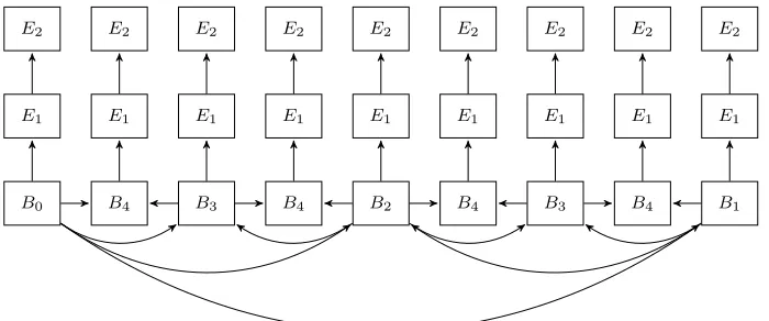
Figure 2.1: Dependency DAG of one GoP with both temporal and quality scalability.

coding) or layer differentiation (e.g., with H.264/SVC coding). In Figure 2.1, we present a DAG for H.264/SVC coding with both temporal and quality scalability [23]. In Figure 2.1, the data segments Bi (0≤i≤4) form a series

of base layers that are compatible with a temporally scalable coding scheme. Segments Ei (i = 1,2) form two enhancement layers that are encoded with

quality-scalability coding based on inter layer prediction. In such a DAG, the edges of the base-layer data represent the data dependency caused by intra-layer motion prediction. The edges between the base and enhancement intra-layers represent the data dependency caused by inter-layer residual differentiation. We note that other dependency structures (e.g., AVC only or spatial layers) can be easily derived as a variation of the structure given in Figure 2.1. For convenience of presentation, in this chapter the same DAG is considered a generalized GoP structure, and is used as the basis of our proposed framework of adaptive resource allocation schemes in the following discussion.

(26)

we consider an empirical rate-distortion model based on the DAG in Figure 2.1. We note that one data unit can only be decoded when all the data units or segments with the higher decoding priority are successfully received. Based on the coding dependencies given by Figure 2.1, we use the operators “” and “” on the set of data types T =B ∪ E, where B={B0, B1, B2, B3, B4} and

E={E1, E2}, to indicate the decoding priority of each data segment. From the DAG, it is straightforward to see the relationsBmBn, EmEn, for all valid

m≤n, and BmEn, ∀m ∈ B, n ∈ E. Noting that the SNR scalability relies

on re-quantizing the residual signal between different SNR layers to obtain quality refinement [23], it is natural to consider that the bitrate of a video layer is controlled by the Quantization Parameter (QP). Letqm and qn be the

QP for the data segments of typem and n (n m, m, n∈ T), and ˜φ(qm) be

the estimated residual Mean Absolute Difference (MAD) of data segmentsm, we adopt the empirical layer-level rate-distortion model proposed in [21]:

   

  

˜

φ(qm) = ˜φ(qn)2a(qm−qn), (2.1.1a)

Dm( ˜φ(qm), qm) =b1log10( ˜φfm(qm)+1)·qm+b2, (2.1.1b)

rm( ˜φ(qm), qm) =cmφ˜gm(qm)2−qm/6. (2.1.1c)

In (2.1.1a), rm is the bitrate for a layer data of type m, and Dm is the

cor-responding distortion measured at the sum of squared differences (SSD). a,

b1, b2, cm, fm and gm are the sequence-dependent parameters, which can be

(27)

2.1.2

Impact of channel coding on distortion model

Since the encoded video is transmitted through an error-prone wireless channel, it is necessary to consider the distortion introduced by error correction and concealment. By introducing the loss probability pi

m when transmitting the

data of layermin GoPi, we first ignore the details of the channel condition and the channel coding schemes, and obtain a generalized model of the expected distortion at the receiver. During the transmission of GoP i, if one of its base layersm∈ B is lost, the decoder will not be able to recover not only the frame that layer m belongs to, but also all the lower-priority frames in the GoP. In this situation, we assume that error concealment for a base layer is performed using the nearest available base layer. We denote the distortion of layer m

after error concealment asDi,ec

n,m, in whichnrepresents the base layer at which

the first decoding error happens in the GoP. If we consider the general case of transmitting layerm (m ∈ T) in GoP i, the expected distortion of layer m

can be expressed as:

Eec{Dim}= P n∈B,nm

Di,ec

n,mpin Q j∈T,jn

(1−pi

j) +Esuc{Dmi } Q j∈T,jm

(1−pi j).

(2.1.2)

In (2.1.2), the first term on the right-hand side accounts for the case when the first error happens at layer n, nm, n∈ B. Considering that the error propagation is confined within a GoP, we adopt the error propagation model in [19] and obtain the following distortion model after error correction:

Di,_n,mec =pi_nσ_e21−knK −1 1 +γkn

, (2.1.3)

in whichK is the frame length of a GoP,knis the frame number counted from

(28)

layer n. σ2

e and γ are the sequence/codec-determined parameters [19]. σe2 is

the variance of the propagated error and can be treated as a constant for each video sequence. γ is the leakage parameter that reflects the efficiency of the spatial filtering of the encoder.

The second term in (2.1.2) accounts for the case when no error happens in transmitting the ancestor base layers of layerm. Esuc{Dmi } is the conditional

expected distortion of layermwhen all its ancestor base layers are successfully received. We can expressEsuc{Dmi } as follows:

Esuc{Dim}=  



Di,ec

m,mpim+Dmi (1−pim), m ∈ B, P

n∈E,nm

Di npin

Q j∈E,jn

(1−pi

j) +Dmi Q j∈E,jm

(1−pi

j), m∈ E.

(2.1.4) In (2.1.4), Di

m is the distortion for data layer m in GoP i (see (2.1.1b)), and

D_m,mi,ce is the distortion after error concealment atm(see (2.1.3)). On the right-hand side of (2.1.4), the first subexpression accounts for the case when layerm

is a base layer. The second subexpression represents the expected distortion when layermis an enhancement layer. The structure of the second subexpres-sion is determined by SVC coding: if an ancestor layern of enhancement layer

m is lost, all the subsequent layers of layer n including m will be abandoned.

2.1.3

Sub-frame level data transmission with HARQ

(29)

state may lead to higher channel error rate and thus higher distortion due to more frequent failure of layer segment transmission (this is reflected by (2.1.2)). Also, when equal protection scheme is adopted, an error occurring in the base layer will have more serious impact on the end-to-end distortion than in the enhancement layer (see (2.1.4)). In order to tackle the first problem of channel-error-induced distortion, we consider the scenario of a non-stationary slowly varying channel, of which the state evolution can be modeled as a finite-state Markov chain [24]. Considering that the hierarchy of the data unit decoding priority is given, we adopt HARQ/FEC for unequal error protection during video streaming.

We consider that Incremental Redundancy-HARQ (IR-HARQ)/FEC based on a family of Rate Compatible Punctured Convolutional (RCPC) codes [24] is adopted for channel error protection of the layer-data segments. Since the packet length of a layer segment is much longer than the single-bit based feed-back signals (namely, ACK and NAK), we assume that the feedfeed-back signal is error-free and immediately ready after the transmission of each data segment. We denote the set of channel state bySc={s1, . . . , s|Sc|}and the RCPC coding

rate byC={c1, . . . , c|C|} (ci> cj if i < j). With RCPC coding, if a NAK is

re-ceived after the transmission with coding rateci, the incremental redundancy

bits will be generated for retransmission by computing the residual bits be-tween codeci and the next target codeci+1.The decoding is performed with a Viterbi decoder that combines the previous and the current set of transmitted bits. We assume that the channel state remains the same during transmission round j for layer n of GoP i as si

n,j. If k retransmissions are supported

be-fore the decoding deadline for layer n of GoP i, then the loss probability pi_n

(30)

is bounded by [24]:

pi

n(ck|sin,1,. . .,sin,k)≤

∞

P d=dfree

X

d1

. . .X

dk

| {z } d1₊_···₊_dk₌_d

ak

d(d1, . . . , dk)×pd(d1, . . . , dk|sin,1, . . . , sin,k).

(2.1.5) In (2.1.5),dis the overall Hamming distance by which the erroneous decoding path deviates from the correct one in the Viterbi decoding trellis and dj _is

the error distance contribution of the j-th additional bits with code cj to d.

ak

d(d1, . . . , dk) is the distance spectra with weightd =d1 +· · ·+dk. pd is the

conditional error probability that a wrong path of distancedis selected by the Viterbi decoder. For hard decision decoding, pd is given by [24]:

pd(d1,. . .,dk|sin,1,. . .,sin,k) = P e1 d1 e1

(_si n,1)

e1₍₁₋

si n,1)

d1₋_e

1_×_{. . .}_×P

ek

dk

ek

(_si n,k)

ek₍₁−

si n,k)

dk₋_e

k_, (2.1.6)

where _si

n,j is the bit error probability (BER) for channel state s

i

n,j. ej is the

number of erroneous bits for thej-th retransmission. For simplicity, we will ig-nore the GoP indexi hereafter. Approximating the value ofpn(ck|sn,1,. . .,sn,k)

with the upper bound in (2.1.5), we obtain the probability of decoding failure for the entire retransmission process after k rounds as:

pf,n(ck|sn,1, . . . , sn,k) = 1−(1−pn(ck|sn,1, . . . , sn,k)) Ln

, (2.1.7)

in which Ln is the number of stages in a trellis for decoding the transmitted

information bits of layern. If we denote the source data length of layern by

ln, then for a code family with a puncture period H, Ln=ln/H.

(31)

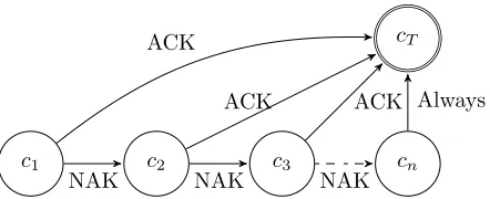
c1 c2 c3 cn

cT

NAK NAK NAK

ACK

[image:31.612.204.425.115.205.2]

ACK ACK Always

Figure 2.2: The state transition for video layer n of GoP i

on the minimum allowable code rate for retransmission1 _{can be determined as}

cn ≥ max(c|C|, ln/(rδn)). According to (2.1.1c), we can determine the length

of each video layer as a function of its QP value as ln = rn( ˜φ(qn), qn)T, in

which T is the duration of one frame. The process of transmitting layer n

can be described by a finite-state machine (Figure 2.2), in which the allowable coding types {c1, . . . , cn} are considered as the states, and cT is the terminal

state when the data is correctly received or the time deadline is reached. Let

k be the index of the maximum allowable code type cn. Then, the expected

transmission time for layer n will be:

E{δn}= k P k=1

δn,k(1−pf,n(ck|sn,1,. . .,sn,k))× k−1

Q j=1

pf,n(cj|sn,1,. . .,sn,j)

+δ_n,k

k Q j=1

pf,n(cj|sn,1,. . .,sn,j).

(2.1.8)

In (2.1.8), we define thatpf,n(c0) = 1. The duration for each channel code type

δn,k is determined as δn,k=ln/(rcn,k).

1_{Here we ignore the situation when} _r _{is not large enough to support the first round}

(32)

2.2

Adaptive Learning for Rate Adaption

2.2.1

Transmission control as a Markov decision

process

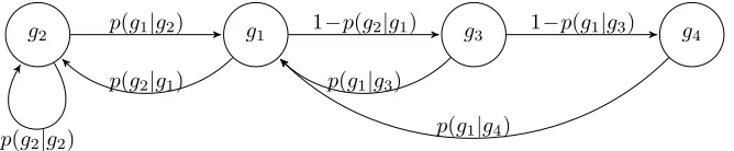
With the rate-distortion model (2.1.2-2.1.4), we can describe the video stream-ing process as a finite-state Markov process (Figure 2.3). In Figure 2.3, state

g1 accounts for the base-layer transmission stage, and stateg2 accounts for the base-layer error concealment stage. The difference between g1 and g2 is due to the data dependency of scalability coding. This is because the decoding error at one base layer will lead to error concealment for the subsequent lower-priority base layers in the same GoP. Thus, the dropping of their respective enhancement layers. In order to differentiate the base-layer types, we defineg1 andg2 as a composition of the layer type and the transmission stage, namely,

g1= (Bi,1) andg2= (Bi,0) (Bi∈ B). Here “1” indicates the data transmission

stage and “0” indicates the error concealment stage. In Figure 2.3, state g3 andg4 account for the transmission stage of the first and the second enhance-ment layer, respectively. For scalability coding, lower-priority (enhanceenhance-ment layer) segments will discarded whenever an error is detected during decoding the higher-priority layer. Therefore, transition probabilities p(g2|g1), p(g1|g3) andp(g1|g4) are equivalent to the probabilities of transmission failure in state

(33)

sum-g1

g2 1−p(g2|g1) g3 g4

p(g2|g1)

p(g1|g2)

p(g2|g2)

1−p(g1|g3)

p(g1|g3)

[image:33.612.157.491.116.185.2]

p(g1|g4)

Figure 2.3: Layered video transmission Markov chain.

marize the transition probabilities of the Markov model in Table 2.1, where

pf,n(cn(g1)|sn) is given by (2.1.7). Here cn(gi) is the smallest channel coding

rate that is used for retransmission in stategi.

Table 2.1: Transition probabilities of the Markov model for layered video transmission

Transition Probability Value

p(g1|g2)

1 if g2= (B4,0), g1= (B0,1), 0 otherwise

p(g2|g2)

0 if g2= (B4,0), g1= (B0,1), 1 otherwise

p(g2|g1) pf,n(cn(g1)|sn)

p(g1|g3) pf,n(cn(g3)|sn)

p(g1|g4) 1

[image:33.612.159.466.341.472.2]

(34)

the cost function is controlled by the QP values and the transmission stages (i.e., error concealment stage or data transmission stage). According to Ta-ble 2.1, the MDP transition probabilities is a function of the channel states, the layer types, the transmission stages and the adopted channel coding rate for IR-HARQ. We also note from the discussion on (2.1.7) that the allowable channel coding rate of one layer is determined by the final code type of its previous layer. Therefore, we can model the MDP by extending the Markov model in Figure 2.3 into a constrained controlled Markov chain. Formally, the constrained MDP is defined as a 5-tuple{S,A, u, v,Pr}:

• S ={S1, . . . , S|S|} is the state space. S =Sc× T × I, where Sc is the

set of discretized channel states, T 3y is the set of the layer types and

I={0,1} 3I is the set of the indicators for the transmission stages. We note that since no error concealment is performed for the enhancement layers, It is only valid when In= 1,∀yn∈ E.

• A = {a1, . . . , a|A|} is the action space. A = C × Q, in which C is the

set of the candidate RCPC code rate that can be used in the maximum round of retransmission. Q is the set of candidate QP values that are chosen according to the SVC coding standard.

• u=Dn(Sn, an) is the instantaneous cost function for transmitting video

layer n:

u(Sn, an) =

Dn(sn, qn, cn), if In= 1,

Dec_m,n(kn(yn)), if In= 0.

(2.2.1)

(35)

accounts for the stages of error concealment of a base layer (see (2.1.3)).

m is the index of the layer used for error concealment (see (2.1.3)).

• v is the constraint on the allowable transmission time for one layer. According to the IR-HARQ scheme (2.1.7-2.1.8), v can be expressed as follows:

v(Sn, an) =δn(sn, qn, cn)−δn (2.2.2)

• Pr = Pr(Sn+1|Sn, an) is the transition probability of the MDP. Based on

Table 2.1, we have:

Pr(sn+1, yn+1, In+1|sn, yn, In, an)

=

    

   

pf,n(cn|sn)p(sn+1|sn), if c1 or c2,

(1−pf,n(cn|sn))p(sn+1|sn), if c3,

1, if c4,c5 or c6,

0, otherwise.

(2.2.3)

According to Table 2.1, the conditions in (2.2.3) is given as:

c1:In= 1, In+1 = 0, yn, yn+1 ∈ B,

c2:In=In+1= 1, yn =E1, yn+1 ∈ B,

c3:In=In+1= 1, yn yn+1,

c4:In=In+1= 1, yn =E2, yn+1 ∈ B,

c5:In= 0, In+1 = 1, yn=B4, yn+1 =B0,

c6:In= 0, In+1 = 0, yn∈ B, yn+16=B0.

Here c1 and c2 account for the transmission failures in the data trans-mission stage. c3 accounts for the transmission success. c4 and c5

(36)

2.2.2

Model-free learning for optimal video streaming

policy

According to (2.2.1-2.2.3), the formulated MDP model is unichain [25]. The goal of transmission scheduling is to find the optimal policy for the MDP that minimizes the long-term average distortion at the receiver. We can express the objective of the constrained MDP given by (2.2.1-2.2.3) as follows:

U = lim

n→∞

1

nEπ

" _n X

m=1

u(Sm, am) #

, (2.2.4)

s.t. C = lim

n→∞

1

nEπ

" _n X

m=1

v(Sm, am) #

≤0,

whereπ is the stationary, randomized policy for taking an action ˜ain state S:

π(˜a) = [Pr(a = ˜a|S) : S ∈ S]. Using Theorems 12.7 from [25], we can obtain the optimal policy for minimizing (2.2.4) by establishing an unconstrained MDP through the Lagrangian approach:

U∗ = min

π sup_λ_≥₀J(π, λ) = sup_λ_≥₀minπ J(π, λ), (2.2.5)

whereλ is the Lagrangian multiplier and J(π, λ) is given by:

J(π, λ) = lim

n→∞

1

nEπ

" _n X

m=1

(u(Sm, am)+λv(Sm, am)) #

. (2.2.6)

Based on (2.2.6), we can define the immediate Lagrangian cost asu(S, a, λ) =

u(S, a) +λv(S, a). According to [22], for a fixed λ there exists a value func-tionV∗(S, λ) for the inner problem in (2.2.5) satisfying the following Bellman equation:

V∗(S, λ)+J∗(λ) = min

a (u(S, a, λ)+ X

S0

(37)

such that the greedy policy π_λ∗ leads to the optimal average cost J∗ over all possible policies π. In order to avoid the inaccuracy due to the adoption of both the empirical distortion model and the unknown transition probabilities, we resort to the technique of R-learning [22] to adaptively approach the value of V∗ and J∗ using the feedback of the immediate cost un(S, a, λ). Based

on (2.2.7), we introduce the action value function Rπ(S, a, λ) of the MDP

following policyπ,

Rπ(S, a, λ) = u(S, a, λ)−Jπ(λ) + X

S0

Pr(S0|S, a)Vπ(S0, λ), (2.2.8)

where Vπ(S0, λ) = minaRπ(S, a, λ), and Jπ(λ) is the average Lagrangian cost

following policy π. Based on (2.2.8), the optimal value of J∗ and Rπ∗(S, a, λ)

is learned iteratively through a two-time-scale learning process as follows [22]:

Rn+1(S, a, λ)←Rn(S, a, λ)(1−βn) +βn

un(S, a, λ)−Jn+min a Rn(S

0_{, a, λ}₎_,

(2.2.9)

Jn+1(λ)←Jn(λ)(1−αn) +αn

un(S, a, λ)+min a Rn(S

0_{, a, λ}₎₋_min

a Rn(S, a, λ)

.

(2.2.10) In (2.2.9) and (2.2.10), βn and αn (0 ≤ βn, αn ≤ 1) are the learning rate for

updating the estimated value ofRnandJn, respectively. Usually, action

explo-ration based on Boltzmann distribution is adopted for policy learning [22]. If so,Jn is updated only when a non-exploratory action is taken. Convergence is

guaranteed for the R-learning process given by (2.2.9-2.2.10), if the conditions

P

nβn =∞, P

nβ

2

n ≤ ∞, P

nαn = ∞, P

nα

2

n ≤ ∞ and limn→∞αn/βn = 0

are all satisfied, and every state/action is visited infinitely often [26].

With the rightmost expression of (2.2.5), we can use a gradient-descent-like algorithm to estimateλ∗ that satisfies the Kuhn-Tucker conditions:

(38)

in whichξn= 1/n is the updating step.

2.3

Simulation Results

In this section, we present a series of numerical simulation results to demon-strate the efficiency of the proposed joint source-channel resource allocation mechanism. In the simulations, a 3-state Markov chain is adopted based on a Rayleigh fading channel model following the discussion of Section II.B in [27]. We assume Binary Phase Shifting Key (BPSK) modulation, so the Bit Error Rate (BER) in (2.1.6) can be determined as s= 1/2 erfc(

p

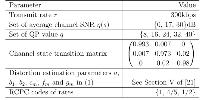
η(s)), where η(s) is the average channel SNR for channel state s [27], and erfc(·) is the com-plimentary Gaussian error function. The family of RCPC code is generated from a parent code with rate 1/2 with memory length of 4. The available coding rate are chosen as {1,4/5,1/2}. The error probability for a layer is estimated based on (2.1.5-2.1.7) following Table III of [24]. Since the source distortion model (1) has been validated by [21], we directly use this synthetic video source in the simulation. The details of the simulation parameters are summarized in Table 2.2.

(39)

[image:39.612.143.485.138.305.2]

Table 2.2: Main parameters used in the video streaming simulation.

Parameter Value

Transmit rate r 300kbps Set of average channel SNR η(s) {0, 17, 30}dB Set of QP-value q {8, 16, 24, 32, 40}

Channel state transition matrix





0.993 0.007 0 0.007 0.973 0.02

0 0.02 0.98





Distortion estimation parameters a,

b1,b2, cm, fm and gm in (1) See Section V of [21]

RCPC codes of rates {1, 4/5, 1/2}

Table 2.3: Retransmission frequencies for the learning processes in Figure 2.4. Initial SNR 0 retransmission 1 retransmission 2 retransmissions 5dB 58.05% 27.10% 14.85% 17dB 86.20% 7.70% 4.05% 30dB 90.85% 4.05% 6.10%

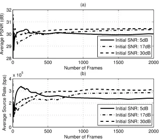
in the same channel condition. Such a discovery helps to explain the difference in the policy evolution for the source-rate adoption in Figure 2.4.(b). With the given channel transition probabilities, a higher initial SNR approximately corresponds to a better channel condition. In Figure 2.4.(b), the transmission with the highest initial SNR reaches the highest average source-coding rate (300kbps), since in a better channel condition, retransmission will be rarely needed. Table 2.3 provides further insight into the policy choosing mecha-nism by summarizing the frequencies of retransmissions for the corresponding learning processes in Figure 2.4.

[image:39.612.121.507.336.401.2]

(40)

✵ ✺ ✵ ✵ ✶ ✵✵ ✵ ✶ ✺✵ ✵ ✷ ✵✵ ✵ ✷ ✷✁ ✸ ✵ ✸ ✶ ✸ ✷ ◆ ✂✄☎ ✆ ✝✞✟✠ ✝✡✄ ✆ ☛ ❆ ☞ ✌ ✍ ✎ ✏ ✌ ✑ ✒ ✓ ✔ ✕ ✖ ✗ ✘ ■ ✚✛ ✜✛✡✢✣◆✤✥✺✦ ✧ ■ ✚✛ ✜✛✡✢✣◆✤✥✶★ ✦✧ ■ ✚✛ ✜✛✡✢✣◆✤✥✸✵✦✧ ✵ ✺ ✵ ✵ ✶ ✵✵ ✵ ✶ ✺✵ ✵ ✷ ✵✵ ✵ ✵ ✶ ✷ ✸ ✹

[image:40.612.157.476.112.388.2]

①✶ ✵ ✩ ◆ ✂✄☎ ✆ ✝✞✟✠ ✝✡✄ ✆ ☛ ❆ ☞ ✌ ✍ ✎ ✏ ✌ ✒ ✪ ✫ ✍ ✬ ✌ ✔ ✎ ✮ ✌ ✕ ✯ ✰ ✱ ✘ ✭☎ ✙ ■ ✚✛ ✜✛✡✢✣◆✤✥✺✦ ✧ ■ ✚✛ ✜✛✡✢✣◆✤✥✶★ ✦ ✧ ■ ✚✛ ✜✛✡✢✣◆✤✥✸ ✵✦ ✧

Figure 2.4: Transmission performance and policy evolution with the proposed adaptive policy learning mechanism. (a) Frame PSNR v.s. frame number. (b) Source-coding rate v.s. frame number.

(41)

[image:41.612.128.498.152.248.2]

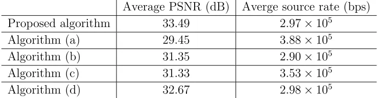
Table 2.4: Performance comparison between different transmission mecha-nisms.

Average PSNR (dB) Averge source rate (bps) Proposed algorithm 33.49 2.97×105

Algorithm (a) 29.45 3.88×105 Algorithm (b) 31.35 2.90×105 Algorithm (c) 31.33 3.53×105 Algorithm (d) 32.67 2.98×105

to the FEC mechanism and 9% when compared to the single-retransmission HARQ mechanism. Table 2.4 also compares the average source coding rates that are reached by each scheme. Comparing the performance of the proposed algorithm with Algorithms (b) and (d), we can see that under the same trans-mit rate constraint, the proposed algorithm is able to provide a higher average PSNR for the same channel condition, when the quality of the encoded video at the transmitter is almost the same.

2.4

Chapter Summary

(42)

(43)

Chapter 3

Learning for Self-organized

Power Allocation in

Heterogeneous Network

As the demand for mobile data traffic continues to grow at an exponential rate, the link efficiency of cellular networks is approaching its fundamental limits. In urban area with densely deployed Macro Base Stations (MBS), the gains of traditional strategies for spectrum efficiency improvement, such as cell-splitting, is significantly reduced due to the severe inter-cell interference. Moreover, the cost of site acquisition in a capacity limited area may also become prohibitively expensive.

(44)

net-work topology with a hierarchical deployment of high-power macrocells and low-power femtocells is known as a HetNet. In practice, the femtocell net-work usually operates underlaying the macrocell netnet-work in a HetNet. This is mainly due to the ad-hoc topology of the femtocells and the lack of coordina-tion between the MBS deployed by an operator and the Femto Access Points (FAPs) randomly deployed by the end users. Consequently, inter-cell/cross-tier interference arises, and interference mitigation with limited coordination becomes essential for preventing performance deterioration in a HetNet.

Due to the random, ad-hoc topology of the femtocells, the FAPs have to operate in a situation of limited information exchange both across tiers (i.e., across macrocells and femtocells) and among the femtocells. Therefore, it is highly desirable that the interference management of the femtocells is fully distributed and self-organized, so that each Femtocell User (FU) is capable of adapting its transmission to the surrounding radio environment with min-imum information exchange. With this in mind, we study an energy-efficient power allocation schemes for an overlay, two-tier HetNet. We note that in the HetNet, conflict of node objectives exists across tiers since a Macrocell User (MU) prefers that the cross-tier interference is minimized, while the FU prefers to transmit at the best Signal-to-Interference-plus-Noise-Ratio (SINR). Considering that private objectives contradict with each other and the means of coordination is lacking, we resort to the game theoretic tools and model the cross-tier, self-centric interactions between different users in the HetNet as a non-cooperative game.

(45)

a number of approaches including the introduction of repetition [30] or exter-nalities (e.g., pricing) [31, 32] were adopted in previous research. As shown by studies on non-hierarchical networks [31–33], choosing a proper pricing mech-anisms with respect to different utility functions can be an efficient way to determine the desired properties of the equilibria.

When it comes to resource allocation in hierarchical networks, such as the femtocell networks and DSA-based CRNs, multi-player Stackelberg game [34] modeling is widely preferred since it is able to reflect the hierarchy and network ad-hoc topology [35, 36] at the same time. The Stackelberg game is characterized by the sequential decision making (namely, follower-leader-based strategy updating), and hence suitable for modeling the heterogeneous user behaviors in the network. To avoid the excessive complexity in modeling the Stackelberg game, most of the existing studies [36–38] assume complete information in the game and favor a problem formulation which is able to lead to a closed-form solution to the Stackelberg Equilibrium (SE). With such assumptions, the SE is usually solved through reformulating the games as hierarchical optimization problems.

(46)

hier-archical networks is usually limited to an uniform learning model [42, 43].

In this chapter, we model the power allocation problem in a two-tier Het-Net from the perspective of the Stackelberg game. In the proposed game model, the MBS behaves as the leader and controls the total cross-tier inter-ference by setting prices to each FU-FAP link. The FU-FAP links behave as the followers and optimize their energy efficiency through interactive power al-location. In order to design an efficient distributed, hierarchical power control scheme with a pricing scheme, we adopt the power efficiency as the main utility metric the FU-FAP link. We then investigate the scenarios of the continuous and discrete power profile of the femtocells, respectively. Due to the compu-tational complexity of obtaining the closed-form solution for the equilibrium, we investigate the property of the proposed game in both the continuous and discrete power profiles, and propose two self-organized strategy-learning algo-rithms for the FU-FAP links in the follower game, respectively. We provide a proof of convergence for the proposed learning schemes in the two follower subgames among the FU-FAP links and propose two corresponding heuristic algorithms to obtain the optimal MBS prices.

3.1

Network Model and QoS Metric

We consider the uplink transmission of a two-tier femtocell network with a single MBS andK FAPs. The MBS and the FAPs share the same bandwidth

(47)

FAPs. For analytical tractability, we suppose that all the channels involved are block-fading and remains constant during each transmission block.

In what follows, we let 0 denote the index of the MU-MBS pair and k ∈ K={1, . . . , K} denote the index of a FU-FAP pair. The channel power gain between transmitter i and receiver j is denoted by hi,j, where i, j ∈ K

S

{0}. The power of transmitter k is denoted by pk and the power vector of all the

FUs is denoted by p = [p1, . . . , pk]. The noise variance for the

transmitter-receiver pair k is denoted by Nk. Then the SINR level at the MBS can be

expressed as:

γ0(p0,p) =

h0,0p0

N0 +

X

k∈K hk,0pk

, (3.1.1)

and the SINR level at the k-th FAP can be expressed as

γk(p0,p) =

hk,kpk

Nk+h0,kp0+

X

j∈K\{k} hj,kpj

. (3.1.2)

During the operation, it is usually beneficial to shift some calls served by the MBS to the FAP. Therefore, we suppose that for the MBS, the require-ment on the femtocell-to-macrocell interference is not rigid. Instead, the MU transmit with a fixed power and to control the interference level, the MBS charges each FU-FAP link for causing interference with a certain price. We denote the vector of interference prices at a time interval by λλλ= [λ1, . . . , λK],

in whichλk is the price for unit interference caused by FU k. The goal of the

MBS is to maximize the total revenue of collected payments from the FU-FAP links:

max

λ λλ

u0=

P k∈K

λkhk,0pk

(48)

For simplicity, in what follows we use the terms FU and the FU-FAP link interchangeably. For the FUs, we assume that each local transmit power pk

is limited by the physical constraint pk ∈ [0, pmaxk ]. The goal of FU k is to

maximize its local net payoff by adaptingpk:

max 0≤pk≤pmaxk

uk =ψ(γk, pk)−λshk,0pk

, (3.1.4)

in whichψ(γk, pk) is the utility function of FUk. We consider that for each FU,

the energy efficiency, namely, the data received per unit energy consumption, is adopted as the the local utility:

ψ(γk,pk) =

Wlog(1 +γk)

pk+pa

, (3.1.5)

where pa denotes the additional circuit power consumption by FU k. We

assume that the local SINR γk can be perfectly measured at the FAP. For the

proposed femtocell network, we suppose that the following assumptions hold:

i) pk is significantly greater than pa;

ii) The femtocell-to-femtocell interference is sufficiently small.

(49)

3.2

Power Allocation Based on Continuous

Stackelberg Game

We model the user interactions in the proposed network as a hierarchical game with the MBS and the FU-FAP links choosing their actions in a sequential manner. When the power allocation of the FUs are given asp, we can define the leader game from the perspective of the MBS as:

Gl =hΛΛΛ,{u0(λλλ,p)}i, (3.2.1) where the MBS is the only player of the game and the action of the player is the price vector λλλ ∈ΛΛΛ.

When the leader action is given byλλλ, we can define the non-cooperative follower game from the perspective of the FUs as:

Gf =hK,P,{uk(λλλ,pk,p−k)}k∈Ki, (3.2.2)

where FU k is one player with the local action pk ∈ Pk.

With each player behaving rationally, the goal of the game (3.2.1) and (3.2.2) is to finally reach the Stackelberg Equilibrium (SE) where both the leader (MBS) and the followers (FUs) have no incentive to deviate. We first assume that the strategies of the FUs and MBS are continuous. Then the SE of the game can be mathematically defined as follows:

Definition 3.2.1 (Stackelberg Equilibrium). The strategy (λλλ∗,p∗) is an SE for the proposed Stackelberg game described by (3.2.1) and (3.2.2) if

u0(λλλ∗,p∗)≥u0(λλλ,p∗),∀λλλ∈ΛΛΛ, (3.2.3)

uk(λλλ∗,p∗k,p

∗

(50)

3.2.1

Femtocell power allocation with continuous

strategies

We start the analysis of the Stackelberg game in (3.2.1) and (3.2.2) by back-ward induction. Suppose that the MBS first sets its strategy as λλλ, then we obtain the non-cooperative follower subgame described by (3.2.2). In order to show the existence of a pure-strategy Nash Equilibrium (NE) in Gf, we

introduce the concept of supermodular game as follows:

Definition 3.2.2 (Supermodularity [34]). A function f :X × T →_R is said to have increasing differences (supermodularity) in (x, t) if for all x0 ≥x and

t0 ≥t,

f(x0, t0)−f(x, t0)≥f(x0, t)−f(x, t).

Definition 3.2.3 (Supermodular game [34,45]). A general normal-form game

hN,{Si}i∈N,{ui}i∈Ni is a supermodular game if for any player i∈ N,

i) the strategy space Si is a compact subset of RK.

ii) the payoff function ui is upper semi-continuous in s= (si,s−i).

iii) ui is supermodular in si and has increasing difference between any

com-ponent of si and any component of s−i.

To show that the proposed follower subgame (3.2.2) is a supermodular game, we introduce Lemma 3.2.1 from [45]:

Lemma 3.2.1. If a function f(s)is twice differentiable, then supermodularity is equivalent to ∂_∂2_sf(s)

i∂sj ≥0 ∀si,sj, j 6=i.

(51)

Theorem 3.2.1. Given the strategy λλλ of the MBS, the follower subgame (3.2.2) is a supermodular game if γk≥pa/pk.

Proof. The first and the second conditions of a supermodular game in Defini-tion 3.2.3 (trivially) holds for the proposed follower subgame (3.2.2). Then, Theorem 3.2.1 can be derived based on Lemma 3.2.1. By taking the component-wise derivative of uk(pk,p−k) with respect to pk, we obtain:

∂uk

∂pk

=−Wlog(1+γk)

(pk+pa)2

+ W Gk (1+γk)(pk+pa)

−λkhk,0, (3.2.5)

in which

Gk =

hk,k

N0+h0,kp0+

P

i∈K\{k}hi,kpi

. (3.2.6)

Then∀k, j ∈ K, k6=j, the value of ∂2uk

∂pk∂pj is given by:

∂2_u

k

∂pk∂pj

= W Hkpk (1+γk)(pk+pa)2

+ W Hkγk (1+γk)2(pk+pa)

− W Hk

(1+γk)(pk+pa)

, (3.2.7)

in which

Hk =

hj,khk,k

N0+h0,kp0+P_i∈K\{k}hi,kpi

2. (3.2.8)

It is easy to verify from (3.2.7) that ∂2uk

∂pk∂pj ≥ 0 if γk ≥ pa/pk. By Lemma

3.2.1, uk has increasing difference between pk and any component of p−k if

γk≥pa/pk. By Definition 3.2.3, the proof of Theorem 3.2.1 is completed.

Given the opponent power allocation p−k, we define the local Best

Re-sponse (BR) of FU k by

ˆ

pk(p−k) = arg max

0≤pk≤pmaxk

uk =ψ(γk, pk)−λshk,0pk

. (3.2.9)

(52)

Proposition 3.2.1. At least one pure-strategy NE exists in the follower sub-game (3.2.2) and the following hold:

i) The set of NEs (3.2.4) has the component-wise greatest element p∗ _and

least element p∗.

ii) If the BRs are single-valued, and each FU uses the BR starting from the smallest (largest) elements of the strategy space to update their strategies, then the strategies monotonically converge to the smallest (largest) NE. iii) If the game has a unique NE, then with any arbitrary initial strategy, the

local myopic BRs converges to the NE.

The properties ofGf given by Proposition 3.2.1 sheds light on the solution

to the local strategy-learning scheme for the FUs. To take advantages of these properties, we introduce the concept of superlevel set and quasiconcavity from [46]:

Definition 3.2.4 (Superlevel Set [46]). Let D denote a convex set in _Rn _and

f :D →_R. The superlevel set of f is defined as Cf(α) = {x∈ D|f(x)≥α}.

Definition 3.2.5(Quasi-Concavity [46]). Following the notation in Definition 3.2.4, function f is quasi-concave on D if ∀α, Cf(α) is a convex set.

(53)

Lemma 3.2.2. Suppose f :D →_R be strictly quasiconcave where D ⊂_RN _is

convex. Then, any local maximum of f on D is also a global maximum of f

on D. Moreover, the set arg max{f(x)|x∈ D} is either empty or a singleton.

Based on Lemma 3.2.2, we are ready to examine the BRs inGf and obtain

Lemma 3.2.3:

Lemma 3.2.3. Given the MBS strategyλλλ, uk is strictly quasiconcave and the

best-response pˆk is single-valued for each FU.

Proof. The proof of Lemma 3.2.3 is derived from investigating the quasicon-cavity of the FU payoff functions. In order to prove Lemma 3.2.3, we first show that the utility function uk in Gf is quasiconcave. We examine the α

-superlevel set of uk(pk, p−k) in pk, which is equivalent to the 0-superlevel set

offα(pk, p−k):

Pk,0 =

pk

fα(pk, p−k)≥0,0≤pk ≤pmaxk ,

fα(pk, p−k) =Wlog(1+γk)−(λkhk,0pk+α)(pk+pa) .

(3.2.10)

We note that fα(pk, p−k) is a concave function, so Pk,α is convex from the

definition of convexity. By the definition of quasiconcavity, ui(λλλ∗, pk, p−k) is

quasiconcave inpk.

Then, we show that ui(pk, p−k) is strictly quasiconcave in pk so the BR

is a global maximum and thus single-valued. Without loss of generality, we consider the power allocation ˆpk∈[0, pmaxk ] with uk(ˆpk, p−k) =α. We assume

that a different power allocation ˜pk satisfies uk(˜pk, p−k)≥uk(ˆpk, p−k).

Corre-spondingly, fα(ˆpk, p−k) = 0 and fα(˜pk, p−k)≥0. Note that for fα(ˆpk, p−k) = 0,

we have:

(54)

in whichGk is given in (3.2.6). The right-hand side of (3.2.11) is a strictly

in-creasing concave function and the left-hand side is a strictly inin-creasing convex function in [0, pmax_k ]. Then the solution to fα(ˆpk, p−k) = 0 is unique in [0, pmaxk ],

so fα(˜pk, p−k)> fα(ˆpk, p−k). Based on the definition of concave function, the

following inequality also holds for 0< δ <1:

fα(δpˆk+ (1−δ)˜pk) ≥δfα(ˆpk) + (1−δ)fα(˜pk)

> fα(ˆpk) = 0.

(3.2.12)

Therefore, the condition for strict quasiconcavity holds asuk(δpˆk+(1−δ)˜pk)>

min (uk(˜pk, p−k), uk(ˆpk, p−k)) = α. Then, Lemma 3.2.3 is a direct conclusion

based on Lemma 3.2.2.

Based on Lemma 3.2.3, we can further prove that the BR of FUk has the following properties, and therefore is a standard function [34]:

i) positivity: ˆpk >0,

ii) monotonicity: for any p0₋_k, p−k ∈ P−k, if p−0 k > p−k, then ˆpk(p0−k) ≥

ˆ

pk(p−k),

iii) scalability: ∀α >1, αpˆk(p−k)>pˆk(αp−k).

For a non-cooperative game whose best-response functions are standard functions, we have the following property in Lemma 3.2.4 [34]:

Lemma 3.2.4. If the best-response functions of a non-cooperative game G are standard functions for all the players, then the game has a unique NE in pure strategies.

(55)

Theorem 3.2.2. Given any MBS strategyλλλ, the follower subgame (3.2.2) has a unique NE if the following condition is satisfied

hk,kpk

Nk+h0,kp0+P_j∈Khj,kpk

≥ pa pk

. (3.2.13)

Proof. Observing (3.1.5), we note that the maximum net-payoff function is lower-bounded by 0 withpk= 0. Since the power vector is always nonnegative,

the positivity property in the BR for each FU k immediately follows Lemma 3.2.3.

We denoteIk(p−k) = (Nk+h0,kp0+

P

j∈K\{k}hj,kpj)/hk,k. Noting thatIk(p−k)

is a strictly increasing function of p−k, monotonicity of ˆpk(p−k) can be

illus-trated by proving that functionpk(Ik) is monotonically increasing inIk. From

(3.2.5) we obtain the necessary condition for pk to be the BR as ∂u_∂pk

k = 0, which

is equivalent to

ω(pk, Ik) =

W(pk+pa)

Ik

−W(1 + pk

Ik

) log(1 + pk

Ik

)

−λkhk,k(pk+pa)2(1 +

pk

Ik

) = 0. (3.2.14)

Since ∂pk

∂Ik =−

∂ω ∂Ik/

∂ω

∂pk, we have

∂ω ∂Ik = 1 I2 k

ξ(pk)+W pklog(1+

pk

Ik

)−W pa

, (3.2.15)

whereξ(pk) = λkhk,k(p2apk+ 2pap2k+p

3

k), and

∂ω ∂pk

=−1 Ik

ζ(pk) +Wlog(1+

p Ik

)

(3.2.16)

where ζ(pk) = λkhk,k(pa+pk)(pa+2Ik+3pk). We note that _∂p∂ω

k < 0, then the

property of monotonicity holds iff _∂I∂ω

k ≥0. With the inequality of logarithmic

function given in [47], log(1 +x)≥x/(1 +x) for x≥ −1, we obtain,

∂ω

∂I ≥

1

I2

ξ(pk)+

W

I +p p

2

k−pa(Ik+pk)

(56)

Therefore, ∂pk

∂Ik ≥0 if p

2

k−pa(Ik+pk)≥0. Then, we obtain the condition for

ˆ

pk(p−k) to be monotonic as:

hk,kpk

Nk+h0,kp0+P_j∈Khj,kpk

≥ pa pk

. (3.2.18)

The proof of scalability is based on Lemma 3.2.3. According to Lemma 3.2.3, there is a one-to-one correspondence between ˆpk and ˆγk. We define

Jk(p−k) = P

j∈K\{k}hj,kpj, then from (3.1.2) the BR can be written as

ˆ

pk(p−k) =

ˆ

γk(N0+h0,kp0+Jk(p−k))

hk,k

. (3.2.19)

From ∂uk

∂pk = 0, we can prove that

∂γk

∂Jk ≤0 following the same procedure as

for proving monotonicity (which is omitted for conciseness). Therefore, γk

is a decreasing function of Jk. Since Jk(p−k) is a standard function [45], we

realize that if α > 1, ˆγk(αp−k) ≤ ˆγk(p−k) and Jk(αp−k) ≤ αJk(p−k). Then,

monotonicity holds for ˆpk(p−k) since

ˆ

pk(αp−k)≤

ˆ

γk(p−k) (N0+h0,kp0+αJk(p−k))

hk,k

≤αpˆk(p−k). (3.2.20)

Therefore, ˆpk(p−k) is a standard function. Based on Lemma 3.2.4, we conclude

that the NE of the follower subgame (3.2.2) is unique.

Remark 3.2.1. If in subgameGf the condition of Theorem 3.2.2 is satisfied,

(57)

We assume that the channel power gainhk,0 is known and the SINRγkcan

be perfectly measured by each FAP. Then, based on Lemma 3.2.3, ˆpk can be

solved locally with the bisection method [46]. Based on Proposition 3.2.1 and Theorem 3.2.2, the asynchronous strategy-updating mechanism defined in [45] can be directly applied toGf. By Proposition 3.2.1, the convergence to the NE

is guaranteed from any arbitrary initial power vector. The strategy-learning algorithm is summarized as Algorithm 3.1:

Algorithm 3.1 Asynchronous strategy updating

Require: each FU sets up an infinite increasing time sequence {Ti

k}k∈K for

scheduling strategy update.

1: for all t ∈ {Ti

k}k∈K do

2: for all k s.t. t={Ti k} do

3: given pt₋−_k1, obtainpt

k = ˆpk(pt−−k1) as in (3.2.9) with bisection.

4: end for

5: end for

3.2.2

Approximate solution to the price of MBS

Now we assume that the strategies of the FUs are given asp from (3.2.9) and consider the leader subgame Gl. For the subgame given by (3.2.1), the local

BR is given by (cf. (3.1.3))

ˆ

λ λ

λ = arg max

λ λ λ0

X

k∈K

λkhk,0pk !

. (3.2.21)

To investigate the solution of (3.2.21), we first consider the feasibility region for λk. We note from (3.2.9) that the maximum value of uk is

lower-bounded by 0 (when pk= 0) and upper-bounded byψ(˜γk,p˜k), where (˜γk,p˜k) =

arg maxψ(γk, pk). Thereby, the price λk charged by the MBS is also

(58)

will stop transmitting and be forced out of the power allocation game. With the aforementioned bound on uk, we look for the constraint on λk in (3.2.9).

However, since uk in (3.2.9) is a transcendental function, it is difficult to

de-rive a closed-form expression of the constraint on λk. Then, the challenge in

analyzing Gl is to find an efficient way to obtain the optimal price ˆλλλ.

By jointly investigating the leader and the follower subgames, we can show that a finite, optimal price ˆλk for each FU coexists with the NE of the follower

subgame.

Theorem 3.2.3. In the Stackelberg game defined by (3.2.1) and (3.2.2), there exists at least one pure-strategy SE with finite price vector λλλˆ from the leader game.

Proof. The proof is based on Theorem 3.2 of [34]. The existence of a pure-strategy SE is guaranteed when each local pure-strategy in the game is compact and convex and the corresponding payoff function is quasiconcave. For the FUs, quasiconcavity of uk(p, λλλ) inpi is given by Lemma 3.2.3. For the MBS,

u0 is an affine function of λλλ, hence it is quasiconcave in λλλ. It is trivial that

p and λλλ are convex and compact, then based on Theorem 3.2 of [34], there exists a pure-strategy NE in the game. Based on our discussion after (3.2.21) on the fact that 0 ≤λk <∞, we can derive the relationship between the BRs

of the FUs and the MBS from ∂uk

∂pk = 0 as:

˜

λk =

WG˜k

hk(1 + ˜γk)(˜pk+pa)

− Wlog(1 + ˜γk) hk(˜pk+pa)2

, (3.2.22)

where ˜pk and ˜γk are the local BR and the corresponding SINR. ˜Gk is given

by (3.2.6) in the proof of Theorem 3.2.1. For (3.2.22), the value of the right-hand side expression is upper-bounded since 0≤ p˜k ≤ pmaxk . Therefore, ˜λk is

(59)

Our approximate solution to the leader subgame is inspired by the pio-neering work [31], which models the asymptotic behaviors of the equilibrium power vector and the corresponding payments. We assume that each FU’s behavior can be asymptotically modeled by two regions, the price-insensitive region and the price-sensitive region. In the price-insensitive region, the FU’s behaviors are hardly influenced by the price. In the price-sensitive region, the local power allocationpkis driven toward 0. We note that the necessary

condi-tion for the NE of the FUs is given by (3.2.22). Asλk→0, the solution of the

BRs in the follower game will be independent of λk and can be approximated

by

(1 +γk) log(1 +γk)−W γk−W Gkpa = 0, k ∈ K, (3.2.23)

where Gk is given by (3.2.6). From Lemma 3.2.3, the solution to (3.2.23) is

unique. Then the payment by FU k will be a linear function of λk, rk =

hk,0pˆkλk.

On the contrary, as λk → ∞, ∀k ∈ K, pk →0. From (3.2.22) we obtain:

hk,kλk(pk+pa) =

W hk,k

Ik+hk,kpk

−Wlog(1 +

hk,kpk

Ik )

(pk+pa)

, (3.2.24)

whereIk is the sum of interference plus noise defined in the proof of Theorem

3.2.2. With pk →0,∀k, (3.2.24) can be approximated as:

hk,kλk(pk+pa)≈

W hk,k

Nk+h0,kp0

. (3.2.25)

and from (3.2.25) we obtain

pk≈

W

λk(Nk+h0,kp0)

−pa. (3.2.26)

(60)

• Low-price asymptote as λk →0:

γ_k∗ ≈γˆk,

rk(λk, pk) =hk,0pˆkλk ∝λk.

(3.2.27)

• High-price asymptote as λk → ∞:

pk≈

W

λk(Nk+h0,kp0)

−pa. (3.2.28)

In (3.2.27), ˜γk is the equilibrium SINR when λk= 0. Since in the low-price

asymptote, rk increases with λk and in the high-price asymptote it decreases

with λk, the maximum payment must happen between the two regions. Then,

we can extend the two FU payment asymptotes toward each other until they meet at the intersection price λa_k. With such an approximation, rk(λak, pk)

will be the maximum payment received from FU k. Combining (3.2.27) and (3.2.28), we can obtain the intersection point for the two asymptotes as:

λa_k ≈ W

(p∗

k+pa)(N +h0,kp0)

, (3.2.29)

where p∗_k is the power allocation corresponding to the SINR γ∗ in (3.2.27).

γ∗ can be obtained by setting λλλ = 0 and solving (3.2.23) with the BR-based asynchronous strategy-updating mechanism.

3.3

Learning for Power Allocation in

Discrete Stackelberg Game

(61)

3.2.2 and 3.2.3) are not satisfied anymore. Therefore, the properties of the game need to be re-evaluated. Within the same game structure for (3.2.1) and (3.2.2), we denote the discrete action set of the FUs byPk={p1k= 0, . . . , p

|Pk|

k }.

It is well known that every finite non-cooperative game has a mixed-strategy NE [34]. For the follower subgame, we define the mixed-strategies of FU k

as πππk= [π1k, . . . , π

|P|

k ], where π j k(p

j

k) = Pr(pk=pjk) is the probability for FU k

to choose the j-th action pj_k ∈ Pk. Then, given any MBS price λλλ, there will

be at least one mixed-strategy NE for the FUs.