This is a repository copy of
Hubbard model as an approximation to the entanglement in
nanostructures
.
White Rose Research Online URL for this paper:
http://eprints.whiterose.ac.uk/10930/
Article:
Coe, J. P., Franca, V. V. and D'Amico, I. orcid.org/0000-0002-4794-1348 (2010) Hubbard
model as an approximation to the entanglement in nanostructures. Physical Review A.
052321. -. ISSN 1094-1622
https://doi.org/10.1103/PhysRevA.81.052321
[email protected] https://eprints.whiterose.ac.uk/ Reuse
Items deposited in White Rose Research Online are protected by copyright, with all rights reserved unless indicated otherwise. They may be downloaded and/or printed for private study, or other acts as permitted by national copyright laws. The publisher or other rights holders may allow further reproduction and re-use of the full text version. This is indicated by the licence information on the White Rose Research Online record for the item.
Takedown
If you consider content in White Rose Research Online to be in breach of UK law, please notify us by
promoting access to White Rose research papers
White Rose Research Online
[email protected]
Universities of Leeds, Sheffield and York
http://eprints.whiterose.ac.uk/
This is an author produced version of a paper published in
PHYSICAL REVIEW A
White Rose Research Online URL for this paper:
http://eprints.whiterose.ac.uk/10930
Published paper
Coe JP, Franca VV, D'Amico I (2010)
Title: Hubbard model as an approximation to the entanglement in nanostructures
81 (5) Article Number: 052321
Hubbard model as an approximation to the entanglement in nanostructures
J. P. Coe1,∗ V. V. Franc¸a2,† and I. D’Amico1‡
1
Department of Physics, University of York, York YO10 5DD, United Kingdom. 2
Physikalisches Institut, Albert-Ludwigs-Universit¨at, Hermann-Herder-Straße 3, D-79104 Freiburg, Germany.
We investigate how well the one-dimensional Hubbard model describes the entanglement of particles trapped in a string of quantum wells. We calculate the average single-site entanglement for two particles interacting via a contact interaction and consider the effect of varying the interaction strength and the interwell distance. We compare the results with the ones obtained within the one-dimensional Hubbard model with on-site interaction. We suggest an upper bound for the average single-site entanglement for two electrons inM wells and discuss analytical limits for very large repulsive and attractive interactions. We investigate how the interplay between interaction and potential shape in the quantum well system dictates the position and size of the entanglement maxima and the agreement with the theoretical limits. Finally we calculate the spatial entanglement for the quantum well system and compare it to its average single-site entanglement.
PACS numbers: 03.65.Ud, 71.10.Fd, 73.21.La, 73.21.Fg
I. INTRODUCTION
Entanglement is considered one of the main resources in quantum information and a reason why quantum computers may be used for computing feats that could not be achieved with traditional processors [1]. In this context quantum dots are thought of as a viable possibility in the quest to construct scalable quantum processors [2–9]. With this in mind, finding accurate ways to calculate the entanglement between electrons in quantum dots becomes important for quantum information processing. However modeling these many-body quantum systems often necessitates the employment of approximations. For example, one-dimensional wells may be used in the study of spherically symmetric quantum dots and aid understanding of trends in more general quantum dot systems [10].
The Hubbard model [11] allows interacting many-body sys-tems to be simulated by mapping them onto a lattice model with (usually) on-site interactions only. Despite its relative simplicity it still captures a significant amount of physics: for example, in strongly correlated fermionic systems it has been used to model particles trapped in an optical lattice [12], highTcsuperconductivity [13], and the metal-insulator
transi-tion [14]. The one-dimensional homogeneous Hubbard model (HM) also benefits from the existence of an exact solution in the thermodynamic limit [15]. Recently the use of the Hub-bard model as an approximation to the exchange coupling in quantum-dot nanostructures has been investigated [16]. The entanglement of the one-dimensional Hubbard model has been investigated in Refs. [17–19]. A local-density approx-imation (LDA) to the entanglement has been proposed in Ref. [20] and applied to inhomogeneous systems.
In this paper we compare the Hubbard model predictions to results from a system of two interacting fermions trapped within a chain of square well potentials. Here each well cor-responds to one of the Hubbard model sites. We consider both
∗Electronic address:[email protected]
†Electronic address:[email protected] ‡Electronic address:[email protected]
repulsive (electron-electron) and attractive interactions, and calculate the corresponding entanglement when the strength of the interaction, the chain length, and the interwell dis-tance are changed. We compare these results with the average single-site entanglement calculated from the Hubbard model. In doing this we infer information on the accuracy of using results from the Hubbard model to approximate the average single-site entanglement of the quantum well system. If the entanglement of electrons in quantum wells can be described using the Hubbard model, then, by using the powerful LDA formalism developed in [20], we could in principle calculate the entanglement present in quantum well systems with a large number of interacting electrons. This would be a non-trivial result as a direct calculation of the entanglement for a system with a large number of interacting electrons becomes compu-tationally prohibitive as the number of particles increases.
In Sec. II we introduce the one-dimensional quantum well system and discuss how we numerically calculate the single-site entanglement. In Sec. III we compare the results from the one-dimensional Hubbard model with the ones from the quantum well system for different interwell distances, chain length, and Coulomb interaction strength. We also investigate how the interaction strength affects the electronic density, and its effect on the matching between the Hubbard and quantum well system. In Sec.IV we propose an upper bound for the average single-site entanglement of the quantum well system and discuss the large Coulomb interaction limit. We investi-gate how close our numerical results come to these analytical expressions. In Sec. V we compare attractive and repulsive particle-particle interaction, as well as discussing the large interparticle attraction limit. Sec. VI is devoted to the com-parison between the average single-site entanglement with the spatial entanglement for the quantum well system and finally Sec. VII contains our conclusions.
II. THE QUANTUM WELL TWO-ELECTRON SYSTEM
2
wells (QWs) is given by
H = X
i=1,2
−1
2
d2
dx2
i
+v(xi)
+CUf(|x1−x2|). (1)
The potentialv(xi)models a string of regularly spaced,
iden-tical square wells, symmetric around the origin, and defined by the quantities:Mthe number of wells,wthe width of each well,dthe barrier width between two consecutive wells, and v0 the depth of each well. We setf(x) = δ(x)to model a
contact Coulomb repulsion and defineCU as the interaction
strength. CU will allow us to compare the system with the
Hubbard model.
We solve the time independent Schr¨odinger equation corre-sponding to Eq. (1) by using ‘exact’ diagonalization; the elec-tronic ground state is a singlet thereby satisfying the stipula-tion of zero magnetizastipula-tion. We calculate the spatial part of the many-body wavefunction using the firstN eigenfunctions of the potentialv(x)as single-particle basis functions. We em-ploy these to produce a basis of symmetric two-particle wave-functions which means we only need to considerN(N+ 1)/2
functions. The form of the Hamiltonian is conducive to this method as by varying the interaction strength independently we do not need to recalculate the basis, or any integral in-volved in the diagonalization, as could be the case if we varied the well geometry directly. In this respect we note that a sys-tem withCU =K, depthv0, well widthwand barrier width
dis equivalent to a system withCU = 1, depthv0/K2, well
widthKw, and barrier widthKd.
A. Average single-site entanglement
We wish to calculate the average single-site (or local) entan-glement of the system ground state. This type of entanentan-glement is relevant for systems of indistinguishable fermions [21]. To this aim we divide our QW system in contiguous ‘sites’, each site centered around a single well.
The entanglement entropySof the system is given by
S= 1
M
M X
i
Si, (2)
with
Si=−T rρred,ilog2ρred,i (3)
the i-site von Neumann entropy of the reduced density ma-trixρred,i. The von Neumann entropy is considered as one
of the definitive measures of entanglement for a pure bipartite system. By dividing the system into sites and moving to a site-occupation basis the reduced density matrixρred,ibecomes a 4×4diagonal matrix [21, 22],
ρred,i=diag[Pi(↑↓), Pi(↑), Pi(↓), Pi(0)] (4)
withPi(γ)the probability of double (γ=↑↓), single (γ=↑or
↓), or zero (γ= 0) electronic occupation at sitei[19].
We calculate the ground-state wave-function, for an even numberM of wells, and from that obtain the occupation prob-abilities. We calculate the probability that both electrons are in the same left-most (Mth) well as
PM(↑↓) =
Z b
−rc
Z b
−rc
|ψ(x1, x2)|2dx1dx2, (5)
whererc is the (numerical) integration cut-off point andb =
−(M/2−1)(w+d)the mid point between the left-most well and the next well.
The probability that only one spin up (or spin down by sym-metry) electron is in this well is
PM(↑) =PM(↓) =
Z b
−rc
Z rc
b
|ψ(x1, x2)|2dx1dx2. (6)
PM(0)may then be deduced, as the probabilities sum to1.
For the other wells the occupation probabilities are
Pj+M/2(↑↓) =
Z b
a
Z b
a
|ψ(x1, x2)|2dx1dx2, (7)
and
Pj+M/2(↑) =
Z b
a
Z a
−rc
|ψ(x1, x2)|2dx1dx2 (8)
+
Z b
a
Z rc
b
|ψ(x1, x2)|2dx1dx2, (9)
with a = −j(w +d) and b = −j(w +d) + d +w,
1 ≤j ≤ (M/2−1). As we only consider an even number of wells distributed symmetrically about the origin, the prob-ability values for wellsM/2to1are known by symmetry.
III. COMPARISON WITH THE HUBBARD MODEL
The Hubbard model [11] is described by the Hamiltonian
HHM=−t X
i,σ
c†i,σci+1,σ+c†i+1,σci,σ
+ ˜UX
i ˆ
ni,↑nˆi,↓, (10)
whereiruns over theM sites andσ=↑,↓. Heretis the hop-ping parameter andU˜ is the interaction strength. c†i,σ (ci,σ)
creates (destroys) a particle of spinσat siteiwhilenˆi,σ =
c†i,σci,σ is the particle number operator. We solve Eq. (10)
by exact diagonalization in the single-site occupation basis {|↑↓i,|↑i,|↓i,|0i}. We apply open boundary conditions and consider an average particle density ofn=n↓+n↑= 2/M,
withnσ the average density of theσ-spin component. Again
we calculate the average single-site entanglement Eq. (2) [17– 19]. Usually the hopping parametert is used to rescale U˜, giving the dimensionless interaction strengthU = ˜U /t.
3
model the hopping parameter is the expectation value of the single-particle operators in the Hamiltonian with respect to the single-particle wave functions localized at adjacent sites. When the hopping parametertis independent of the sites it may be written as
t=hφi(r)|
−1
2∇
2+V(r)
|φi+1(r)i, (11)
whereφi is the wavefunction at any site i andV(r) is the
single-particle confining potential.
Following this definition, we estimate the hopping parame-ter for our quantum well model as
tw=hφL(x)|
−1
2
d2
dx2 +v(x)
|φR(x)i, (12)
whereφL(R)has the shape of the single-particle ground state
of the finite single square well potentialφw, but centered in
the left (φL) or right (φR) well. Herev(x)is the potential
de-fined in Eq. (1), with the zero of energy chosen such thatv(x)
has zero as its lowest value thereby ensuring that the potential contribution is always positive and an increase in the depth of the well causes the hopping parameter to decrease. The phase ofφLandφRis chosen to maketwreal and positive.
The on-site interaction in the Hubbard model [11] is defined by
˜
U =1
2hφi(r2)| hφi(r1)|
1
|r1−r2||φi(
r1)i |φi(r2)i. (13)
The corresponding parameter in our 1D model with a delta function interaction is then
˜
Uw=
CU 2
Z
φ4w(x)dx. (14)
We may now estimateU for our model as
U ≈ U˜w tw
. (15)
For systems of wells characterized by the parametersw=d= 2a0, wherea0is the (effective) Bohr radius, andv0= 10
(ef-fective) Hartree, we findU = 12344CU; when the interwell
distance is reduced tod= 0.2a0we obtainU = 3.14CU, and
U = 1.27CU for the limiting cased= 0.
A. Effect of many-body interactions on the electronic density
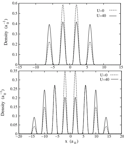
Next we explore how the electron density alters to maxi-mize its exposure to the attractive confining potential whilst attempting to minimize the interaction between the electrons. For two wells the density profile is clearly symmetric so we do not discuss it further. A non-interacting four well system (upper panel of Fig. 1, dashed line) displays a density clearly higher in the inner wells. However for U = 40, due to the electron repulsion, the difference between the electron den-sity in the inner and outer wells becomes much smaller (solid
−1 0
Density (a )
−1 0
Density (a )
x (a )0
0.6
0.5
0.4
0.3
0.2
0.1
0
−15 −10 −5 0 5 15
0.35
0.3
0.25
0.2
0.15
0.1
0.05
0
15 10 5 0 −5 −10 −15 −20
U=40 U=0 U=40 U=0
10
[image:5.595.339.541.50.285.2]20
FIG. 1: Upper Panel: electron density forU = 0(CU= 0) (dashed
line) andU = 40(CU= 0.00324) (solid line) for a4well potential
andw= 2a0,d= 2a0andv0 = 10Hartree. Lower Panel: as for
the upper panel but for a system of8wells.
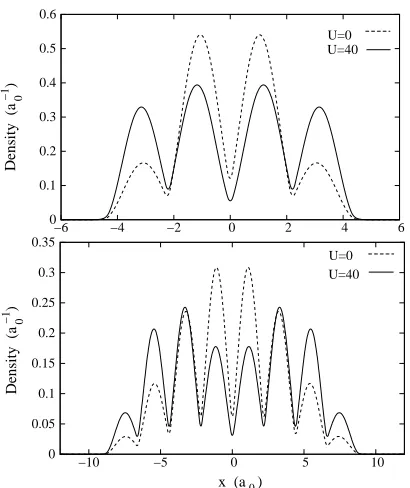
line). For eight wells andU = 0the inner wells are again preferentially occupied while there is very little density in the outermost wells (Fig. 1, lower panel, dashed line). When the interaction is ‘switched on’ toU = 40the two central wells have a lower peak density than the nearby wells to compen-sate for the Coulomb repulsion, but the outermost wells still display, by comparison, a much lower density. Similar behav-iors of the interacting and non-interacting densities are found when the distance between wells is reduced by an order of magnitude (d= 0.2a0). However in this case the density is
considerably different from zero in the barrier region (Fig . 2). These results seemingly show that, apart from accidental compensation, the electron density in the different wells can not be made equal by applying an unmodulated Coulomb in-teraction.
B. Comparison of entanglement results
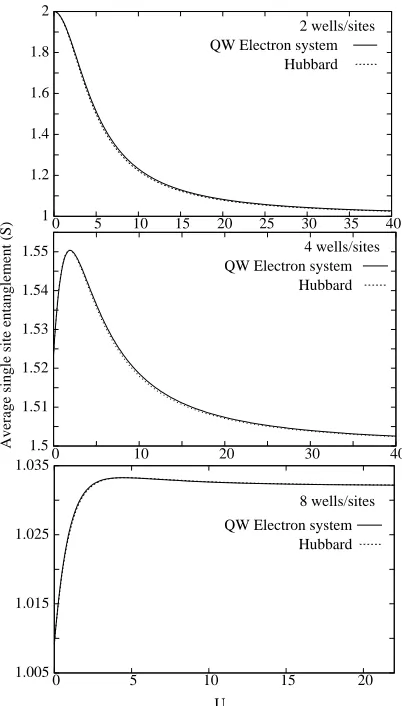
In Fig. 3 we compare the average single-site entanglement for the Hubbard model with that of the QW electron systems characterized byd= 2,d= 0.2, and the limiting cased= 0. The latter corresponds to the arbitrary partition of a single well of widthM wintoMequal regions.
Ford= 2a0 and two wells (upper panel) we see that the
4
−1 0
Density (a )
−1 0
Density (a )
x (a )0
0.35
0.3
0.25
0.2
0.15
0.1
0.05
0
−10 −5 0 5 10
U=0 U=40 0.3
U=40 U=0 0.6
0.5
0.4
0.2
0.1
0
[image:6.595.75.280.48.292.2]−6 −4 −2 0 2 4 6
FIG. 2: Upper panel: electron density forU = 0(CU = 0) (dashed
line) andU = 40(CU = 12.75) (solid line) for a4well potential
withw= 2a0,d= 0.2a0andv0 = 10Hartree. Lower Panel: as
for the upper panel but for a system of8wells.
two systems is almost indistinguishable.
Ford= 0.2a0, two wells, andU .8the Hubbard model
is fairly accurate in reproducing the average single-site en-tanglement, while, for stronger interactions, results from the Hubbard model reproduce only the qualitative trend (Fig.3, upper panel). ForU &8the entanglement values are interme-diate between the Hubbard model and the limiting cased= 0: in this respect we note that ford= 0.2a0even when the
re-pulsive interaction is as high asU = 40(CU = 12.75) the
electron density in the QW system does not become localized within the wells (see Fig. 2).
When four wells are considered, the Hubbard model repro-duces the entanglement trend qualitatively and is less accurate when the interaction is low (Fig. 3, middle panel). The max-imum entanglement is lower ford = 0.2 a0 and in general
the entanglement trend is intermediate between the Hubbard model and the limiting cased= 0. For four wells the differ-ence between the maximum values of the entanglement can not be removed by rescaling U (see discussion in next sec-tion).
For eight wells the Hubbard model reproduces the qualita-tive behavior but the entanglement is lower at all values ofU and intermediate with respect to the results ford= 0.
It should be noted however that, even ford = 0.2a0, the
percentage error for the entanglement as estimated using the Hubbard model will be relatively small for the eight and four well systems (∼1%), while more substantial for the two-well case andU &8(∼20%).
Our results show that the average single-site entanglement of the Hubbard model is a very good match for the
entangle-Average single site entanglement (S)
U
Four wells/sites Two wells/sites
Eight wells/sites 1.44
1.48 1.52 1.56
0 10 20 30 40
1 1.2 1.4 1.6 1.8 2
0 10 20 30 40
0.97 0.99 1.01 1.03
Hubbard QW Electron system d=0 QW Electron system d=0.2 QW Electron system d=2
Hubbard QW Electron system d=0 QW Electron system d=0.2 QW Electron system d=2
25 20 15 10 5
0
[image:6.595.337.539.49.391.2]Hubbard QW Electron system d=0 QW Electron system d=0.2 QW Electron system d=2
FIG. 3: Average single-site entanglement for the Hubbard model and the QW electron system withU = ˜Uw/tw,w = 2a0,d = 2a0,
d= 0.2a0ord = 0, andv0 = 10Hartree. Upper panel: 2sites
withn= 1a−1
0 and2wells. Center panel:4sites withn= 0.5a
−1 0
and4wells. Lower panel:8sites withn= 0.25a−1
0 and8wells.
ment of a QW electron system when wells are far enough apart to prevent significant electron density in the interwell barrier region (see Fig. 1); it is less good, although it gives the gen-eral trend, when the wells become closer, as the density profile displays less well-defined ‘sites’ (see Fig. 2) . Surprisingly though, when considering a large number of wells, the Hub-bard model reproduces the entanglement within few percent at all interaction strengths, even when compared to the limiting case scenariod = 0(Fig.3, lower panel). This results sug-gests that here the Hubbard model sites could be interpreted as a fine enough mesh discretization of the continuous spatial variable.
C. RescalingU˜w/tw
We now investigate whether, for d = 2a0, the small
dis-crepancy between the Hubbard model and the QW system re-sults for the entanglement may be removed by choosing an ‘ad hoc’ value ofU˜w/(twCU).
5
for the QW system is almost identical to the results from the Hubbard model for all the systems considered (Fig. 4).
U
Average single site entanglement (S)
8 wells/sites 4 wells/sites 2 wells/sites
15 Hubbard
0 5 10 20
1.005 1.015 1.025
1.035 0 10 20 30 40
QW Electron system Hubbard QW Electron system Hubbard QW Electron system
1.55
1.54
1.53
1.52
1.51
1.5 1 1.2 1.4 1.6 1.8 2
[image:7.595.75.276.87.440.2]0 5 10 15 20 25 30 35 40
FIG. 4: Average single-site entanglementS for the Hubbard model and the QW electron system withU = 11500CU,w= 2a0,d= 2
a0, andv0 = 10Hartree. Upper Panel:2sites withn= 1a− 1 0 and
2wells. Center Panel:4sites withn= 0.5a−1
0 and4wells. Lower
panel:8sites withn= 0.25a−1
0 and8wells.
This suggests that although the calculatedU˜w/tw gives a
good estimate for the parameter U to be used in the Hub-bard model, we may improve the entanglement accuracy by fittingU˜w/(CUtw)and thereby compensate for some of the
differences between the models. The extent of the scaling confirms that—at least for parameters for which there is no significant electron density in the barrier regions—the use of a single square well wave-function is a good approximation in the calculation ofU˜w/twas the result is very close to the
scaled value.
IV. UPPER BOUND FOR THE ENTANGLEMENT AND STRONG COULOMB INTERACTION LIMIT
Let us consider the case of zero magnetization, i.e.P(↑) =
P(↓)and2N particles whereN is an integer. WithM wells,
we then have a constraint from conserving the particle number
φ= M X
i
(Pi(↑↓) +Pi(↑))− N = 0, (16)
and constraints from the requirement that occupation proba-bilities for any well/site must sum to one
ψi=Pi(↑↓) + 2Pi(↑) +Pi(0)−1 = 0. (17)
We use Lagrange multipliers to maximizeSsubject to these constraints, i.e.
∂ ∂Pi(γ)
S−λφ−
M X
j
µjψj
= 0 (18)
withγ =↑,↑↓,0. Eliminatingλ andµi from the resulting
equations give
Pi(↑↓)Pi(0) = (Pi(↑))2. (19)
Eq. (19) relates occupation probabilities within each site, so we can find a local maximum of the entanglement where all the wells/sites are equivalent, i.e. Pi(γ) = P(γ).
Im-posing this condition on Eqs. (16), (17) and (19) gives
P(↑) =N/M−(N/M)2andP(↑↓) = (N/M)2. We note
that it is only the ratioN/M that matters for the probabilities and hence the entanglement. For 2 particles, the largest entan-glement occurs for two well/sites (Fig. 3); this suggests that N/M = 1/2(half-filling) may be the condition to obtain the largest maximum for the entanglement.
We now continue with N = 1 and note that
P(↑) = 1/M−1/M2andP(↑↓) = 1/M2correspond to the
condition of no preferred well and two uncorrelated particles of opposite spin.
Reduced density matrices with eigenvalues equal to 1/g, g the number of degrees of freedom, would correspond to maximal entanglement. However, under the stipulation of preserving the particle number together with the request that
P
γPi(γ) = 1, this state cannot be achieved except for
M = 2. We could think of moving closer to this by attempt-ing to achieve reduced density matrices with more homogene-ity within the eigenvalues, i.e., achievingPi(γ)≈Pi(γ′), at
least within certain wells. We implement this by relaxing the condition that the wells are equivalent and moving part of the particle density from one site to another. We reducePi(↑)and
Pi(↓)byqwhile increasing Pj(↑↓)at sitej 6= ibyq, with
the empty occupation probabilities adjusted accordingly. Set-tingdS/dq = 0givesq = 0suggesting that the maximum entanglement occurs when all wells are equivalent.
Under this condition, the average single-site entanglement is given by Eq. (3), and simplifies to
Sth
max(M) = 2 log2(M) + 2
1
M −1
log2(M−1). (20)
This maximum average single-site entanglement decreases as the number of wells increase (see Table I) and, for two
parti-cles,Sth max
M→∞
6
M Sth
max Smax
2 2 2
[image:8.595.383.495.48.122.2]4 1.623 1.550 6 1.300 1.234 8 1.087 1.033
TABLE I: Table showing the maximum theoretical average single-site entanglement Eq. (20), and the maximum entanglement as calcu-lated for the QW electron system ford= 2a0and different numbers
of wells.
correspond to the limit of the number of sites going to infin-ity and the average particle densinfin-ity going to zero. This limit would in fact be expected to have no entanglement as it is es-sentially a product state of empty occupations.
Ford = 2a0,Smaxth is reached forU = 0 and two wells,
similarly to the Hubbard model; however, forM > 2, some interaction is required to balance the propensity of the non-interacting wave-function to favor inner wells. Turning on the repulsion between electrons will tend to reduce the discrep-ancies between the electron density peaks in different wells (see e.g. the upper panel of Fig. 1); however this will also tend to decrease the double occupation probability and in par-ticular the already too low value of P1(M)(↑↓)at the outer
wells. Therefore, due to the open boundary conditions here considered, it may not be possible for the system to reach the theoretical maximum for the entanglement by simply varying U, as a perfect balance between occupation probabilities in different wells may not be achieved without, for example, a spatial modulation of the particle-particle interaction.
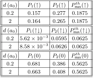
d(a0) P1(↑) P2(↑) Pmaxth(↑)
0.2 0.157 0.277 0.1875 2 0.164 0.265 0.1875
d(a0) P1(↑↓) P2(↑↓) Pmaxth(↑↓)
0.2 5.62×10⁻³
0.0595 0.0625 2 8.58×10⁻³
0.0626 0.0625
d(a0) P1(0) P2(0) Pmaxth(0)
[image:8.595.142.211.49.121.2]0.2 0.681 0.386 0.5625 2 0.663 0.408 0.5625
TABLE II: Occupation probabilities forM = 4, interwell distances
d= 0.2a0andd= 2a0, and interaction valueUSmax
correspond-ing to the entanglement maximum. Theoretical values as used in Eq. (20)
In Table II we compare the occupation probabilities Pth
max(γ)corresponding to the maximum theoretical
entangle-mentSth
max to the occupation probabilities calculated for the
maximum value of the entanglement for theM = 4system and interwell distancesd= 2andd= 0.2. We note that the largest discrepancy with the theoretical values is observed for the double occupation probability, withP1(↑↓)≪Pmaxth (↑↓).
This is greatly responsible for the fact thatSmax < Sthmaxfor
both interwell distances. Thed = 0.2 system also presents the largest discrepancies|Pi(γ)−Pmaxth (γ)|for anyγandi, as
M Sth
U→∞ SU=40 SU=450
2 1 1.030 1.000 4 1.5 1.503 1.500 6 1.252 1.226 1.226 8 1.061 1.032 1.032
TABLE III: Table showing the limiting value for the average single-site entanglement entropy Eq. (21), and the results from the QW elec-tron system withU = 40andU = 450ford= 2a0and different
numbers of wells.
well as a large inhomogeneity between well occupation prob-abilities|P1(γ)−P2(γ)|for anyγ. These account for the fact
that this system presents a lower maximum for the entangle-ment in respect to the system withd= 2a0.
We may calculate the theoretical limit for the entanglement of two electrons andMwells whenU → ∞and all wells are equally favorable. Using a similar procedure to section IV but
withP(↑↓) = 0andP(↑) =P(↓) = 1/M, we obtain
Sth U→∞=
2
M log2(M) +
2
M −1
log2
1− 2
M
. (21)
We see in Table III that Eq. (21) describes the largeU limit of the QW system fairly well, with a percentage error of at most 3%. ForM = 6 andM = 8the entanglement of the QW system saturates atU ≈40and remains slightly below the theoretical limiting value as in this case the assumption of equivalent wells does not hold even for very strong interac-tions (Fig. 1, lower panel).
d(a0) P1(↑) P2(↑) Pth(↑)
0 0.196 0.284 0.25 0.2 0.228 0.268 0.25 2 0.249 0.251 0.25
Hubbard 0.249 0.251 0.25
d(a0) P1(↑↓) P2(↑↓) Pth(↑↓)
0 2.04×10⁻⁴
1.81×10⁻²
0 0.2 2.12×10⁻⁴
3.46×10⁻³
0 2 6.80×10⁻⁷
5.87×10⁻⁶
0
Hubbard 4.94×10⁻⁷
4.43×10⁻⁶
0
d(a0) P1(0) P2(0) Pth(0)
0 0.608 0.414 0.5 0.2 0.544 0.461 0.5 2 0.501 0.499 0.5
Hubbard 0.501 0.499 0.5
TABLE IV: Occupation probabilities forM = 4, interwell distances
d= 0,d= 0.2a0andd= 2a0, andU = 450. The
correspond-ing values for the Hubbard model are reported as well. Theoretical values as used for Eq. 21.
[image:8.595.101.252.419.547.2]theo-7
retical limiting results and theM = 4system. We consider d= 0,d = 0.2a0,d= 2a0, and the results from the
Hub-bard model. Table IV shows that the occupation probabilities ford = 2a0are almost identical to the Hubbard model and
extremely close to the theoretical limiting values. Ford= 0.2
instead, no matter how strong the Coulomb repulsion between particles is made (U = 450in the table), the very narrow in-terwell barriers fail to counteract the effect of the boundary conditions, which favor occupation in the central wells. In general the inhomogeneity between well occupation probabil-ities|P1(γ)−P2(γ)|increases for decreasingd, underlining
the fact that the definition of ’sites’ become more arbitrary. However the substantially larger double occupancy probabil-ity encountered ford < 2increases the available degrees of freedom and hence the entanglement. This confirms the en-tanglement trend observed in Fig. 3, center panel.
V. ATTRACTIVE VERSUS REPULSIVE PARTICLE-PARTICLE INTERACTION
We wish to discuss how the entanglement pattern is modi-fied when we compare attractive (CU, U <0) with repulsive
[image:9.595.336.540.52.176.2]particle-particle interaction. In the following we will consider the QW system withd = 2a0and the Hubbard model. In
Fig. 5 we show the change in the average single-site entan-glement with U for different numbers of wells. From our calculationsSmax always occurs forU ≥ 0and corresponds
toU = 0 for two, U = 2.1 for four, whileU = 4.8 for eight wells. As expected from Eq. (20), the maximum aver-age single-site entanglementSmax decreases with increasing
number of wells and our conjectured theoretical maximum entanglementSth
max is indeed an upper bound, to which the
actual system comes reasonably close (Table I). ForM >2, due to the non-periodic nature of the system, an unmodulated interaction strength drives the system towards having equiv-alent wells only in the very large |U| limit. However, as particle-particle interaction would naturally introduce corre-lations, any spatial modulation ofU should probably be non trivial in order to mimic the uncorrelated electrons’ occupa-tion probabilities corresponding to the maximum theoretical entanglement Eq. (20).
ForU < 0the entanglement decreases monotonically for increasing|U|. This is due to a disproportionate increase of the double occupation probabilities, which are favored by the attractive interparticle interaction. This limits the access to other degrees of freedom which might contribute to the entan-glement, and consequently the entanglement is reduced.
Our calculations show that the Hubbard model reproduces well the average single-site entanglement of a QW system with relatively wide interwell barriers. The comparison for M = 4is shown in Fig. 5.
A. Large inter-particle attraction limit
ForU <<0the two center wells could have equal proba-bilities of double occupation and emptiness whilst all the other
U
Average single site entanglement (S) 0.4−40 −20 0 20 40 0.8
1.2 1.6 2
QW system 8 wells QW system 2 wells QW system 4 wells Hubbard 4 sites
FIG. 5: Average single-site entanglement of the 4-sites Hubbard model and of the QW system with2, 4, and 8wells vs U, U =
˜
Uw/tw,d= 2a0,w= 2a0, andv0= 10Hartree.
M Sth,1
U <<0 S
th,2
U <<0 SU=−40
2 1 1 1.030 4 0.5 0.811 0.706 6 0.333 0.65 0.585 8 0.25 0.544 0.497
TABLE V: Table showing the theoretical limits for the average single-site entanglement andU ≪0for different numbers of wells. Results from the QW system withd = 2a0 and U = −40are
presented as well.
wells would be empty. This would lead to an average single-site entanglement of
SU<<th,1 0= 2/M. (22)
We see in Table V that the QW system does not get very close to this limit except forM = 2. The form of the confining po-tential is such that all the wells will always contain some den-sity for the finite interaction strengths considered (U ≥ −40). At these interaction strengths the system is better described by assuming that all wells are equivalent but that there is no single occupation. This gives
SU<<th,2 0= 1
M log2(M)−
1− 1
M
log2
1− 1
M
. (23)
Fig. 5 shows that the entanglement remains intermediate be-tweenSU<<th,1 0andSth,U<<2 0, due to the relatively limited effect of the short-range interaction considered.
VI. SPATIAL VERSUS AVERAGE SINGLE-SITE ENTANGLEMENT
[image:9.595.382.497.231.302.2]8
the reduced density matrix,Ssp=−T rρred,splog2ρred,sp, with
ρred,spcalculated from the spatial degrees of freedom as [23]
ρred,sp(x1, x2) =
Z
Ψ∗(x
1, x3)Ψ(x2, x3)dx3. (24)
This expression is diagonalized with respect to the basis set employed. Also in this case we allow for attractive as well as repulsive interaction between the particles.
Notice that in the present case the spatial entanglement is zero when there is no interaction as the wave-function fac-torizes into spatial and spin components and the implicit cor-relations arising from the Pauli exclusion principle—and the related entanglement—are accounted for within the spin de-grees of freedom.
For two wells (Fig. 6, upper panel) we see that the spatial entanglement is a mirror image of the site entanglement when reflected along the lineS, Ssp = 1. For larger numbers of
wells the relationship is more complicated. In most regions when the spatial entanglement increases the site entanglement decreases and vice versa; however the spatial entanglement does not have a minimum exactly where the average single-site entanglement has a maximum. This is because the spatial entanglement’s minimum always occurs atU = 0when there is no correlation between the particles’ positions.
An intuitive explanation for the almost opposite behavior of these two types of entanglement is that forU >0increasing U increases the repulsion and the correlation between parti-cles. Hence one electron’s position reveals more about the other electron while the number of spatial degrees of free-dom is not dramatically limited, so the spatial entanglement increases. However the probability of double occupation is reduced by a large positive interaction so less is learned by measurement with respect to wells/sites even though the elec-tron affects the other’s position more. Therefore the site en-tanglement decreases once it has reached its maximum but, forM >2, much less strongly than the spatial entanglement’s increase.
ForU <0the reduction in the probability of single occu-pation causes the average single-site entanglement to decrease markedly when|U|increases. The increase in spatial entan-glement with increasing|U|here comes from the system ap-proaching the situation where measurement of one electron’s position reveals the other electron to be in the same region. This results in large entanglement and we find that the spa-tial entanglement forU <0increases as the number of wells where the electron can be found increases.
VII. CONCLUSION
In this paper we examined the average single-site and spa-tial entanglement of two particles confined in a string of quan-tum wells and interacting via a contact interaction. The re-sults for average single-site entanglement were compared to those of the one-dimensional Hubbard model with on-site in-teraction, to investigate when this model is a good approxi-mation to the two-particle system. For repulsive (Coulomb) interaction, we found that the trend of the entanglement was
2 wells
4 wells
8 wells
U
sp
Entanglement (S, S )
Spatial
Spatial
Spatial
−10
−20 0 10 20
2.5
2
1.5
1
0.5
0 2
0 0.4 0.8 1.2 1.6 0 0.5 1 1.5
Average single site
Average single site
[image:10.595.335.542.48.393.2]Average single site
FIG. 6: Average single-site entanglementSand spatial entanglement
Sspfor the QW electron system withU= ˜Uw/tw,d= 2a0,w= 2
a0,v0= 10Hartree and2wells (upper panel),4wells (center panel),
and8wells (lower panel)
reproduced, with a generally good quantitative agreement, when comparing with a Hubbard model characterized byU =
˜
Uw/tw whereU˜w andtw were calculated from the quantum
9
counteract the propensity of the particles to occupy the inner wells.
Despite the calculated values of U˜w andtw appearing to
give very good results for relatively wide interwell barriers, we found that an even better match between the Hubbard model and the electron system could be achieved by rescaling the value ofU˜w/(CUtw). This suggests that there were some
small contributions to the interaction beyond the on-site repul-sion for the chosen well parameters, but that the main approxi-mation used—hopping parameters and interaction strength in-dependent of the site and estimated from the ground state of a single finite quantum well—remains valid. However, as the interwell barrier width decreases, these approximations fails and no rescaling ofU˜w/(CUtw)could improve the match
be-tween the quantum well system and the Hubbard model re-sults.
We also considered an attractive interactionU <0and rel-atively wide interwell barriers. In this case the average single-site entanglement of the quantum well system was well ap-proximated by the Hubbard model.
Finally we have considered a different type of entanglement—the spatial entanglement—for the quantum well system. Our results showed that the spatial entanglement tends to display in most parameter regions an opposite trend in respect to the average single-site entanglement.
Future work includes considering long range Coulomb in-teractions, and how this affects comparison with the results from the Hubbard model.
[1] M. A. Nielsen and I. L. Chuang, Quantum Computation and
Quantum Information (Cambridge University Press, 2000).
[2] G. Chen, N. H. Bonadeo, D. G. Steel, D. Gammon, D. S. Katzer, D. Park, and L. J. Sham, Science 289, 1906 (2000).
[3] T. E. Hodgson, M. F. Bertino, N. Leventis, and I. D’Amico, Journal of Applied Physics 101, 114319 (2007).
[4] M. Feng, I. D’Amico, P. Zanardi, and F. Rossi, Europhys. Lett.
66, 14 (2004).
[5] T. P. Spiller, I. D’Amico, and B. W. Lovett, New J. of Phys. 9, 20 (2007).
[6] A. Imamo¯glu, D. D. Awschalom, G. Burkard, D. P. DiVincenzo, D. Loss, M. Sherwin, and A. Small, Phys. Rev. Lett. 83, 4204 (1999).
[7] X. Li, Y. Wu, D. Steel, D. Gammon, T. H. Stievater, D. S. Katzer, D. Park, C. Piermarocchi, and L. J. Sham, Science 301, 809 (2003).
[8] D. Loss and D. P. DiVincenzo, Phys. Rev. A 57, 120 (1998). [9] I. D’Amico and F. Rossi, Appl. Phys. Lett. 79, 1676 (2001). [10] S. Abdullah, J. P. Coe, and I. D’Amico, Phys. Rev. B 80,
235302 (2009).
[11] J. Hubbard, Proc. R. Soc London. Series A 276, 238 (1963).
[12] G. Xianlong, M. Polini, M. P. Tosi, V. L. Campo, Jr., K. Capelle, and M. Rigol, Phys. Rev. B 73, 165120 (2006).
[13] M. Machida, S. Yamada, Y. Ohashi, and H. Matsumoto, Physica C: Superconductivity 445-448, 90 (2006).
[14] T. Paiva and R. R. dos Santos, Phys. Rev. B 58, 9607 (1998). [15] E. H. Lieb and F. Y. Wu, Phys. Rev. Lett. 20, 1445 (1968). [16] J. Pedersen, C. Flindt, N. A. Mortensen, and A. P. Jauho, Phys.
Rev. B 76, 125323 (2007).
[17] S.-J. Gu, S.-S. Deng, Y.-Q. Li, and H.-Q. Lin, Phys. Rev. Lett.
93, 086402 (2004).
[18] V. V. Franc¸a and K. Capelle, Phys. Rev. A 74, 042325 (2006). [19] D. Larsson and H. Johannesson, Phys. Rev. Lett. 95, 196406
(2005).
[20] V. V. Franc¸a and K. Capelle, Phys. Rev. Lett. 100, 070403 (2008).
[21] P. Zanardi, Phys. Rev. A 65, 042101 (2002).
[22] D. Larsson and H. Johannesson, Phys. Rev. A 73, 042320 (2006).