This is a repository copy of Bayesian network learning with cutting planes.
White Rose Research Online URL for this paper:
http://eprints.whiterose.ac.uk/76731/
Version: Submitted Version
Proceedings Paper:
Cussens, James orcid.org/0000-0002-1363-2336 (2011) Bayesian network learning with
cutting planes. In: Cozman, Fabio and Pfeffer, Avi, (eds.) Proceedings of the 27th
Conference on Uncertainty in Artificial Intelligence (UAI 2011). 27th Conference on
Uncertainty in Artificial Intelligence, 14-17 Jul 2011 AUAI Press , ESP , pp. 153-160.
[email protected] https://eprints.whiterose.ac.uk/
Reuse
Items deposited in White Rose Research Online are protected by copyright, with all rights reserved unless indicated otherwise. They may be downloaded and/or printed for private study, or other acts as permitted by national copyright laws. The publisher or other rights holders may allow further reproduction and re-use of the full text version. This is indicated by the licence information on the White Rose Research Online record for the item.
Takedown
If you consider content in White Rose Research Online to be in breach of UK law, please notify us by
Bayesian network learning with cutting planes
James Cussens
Dept of Computer Science & York Centre for Complex Systems Analysis University of York, Deramore Lane, York, YO10 5GH, UK
Abstract
The problem of learning the structure of Bayesian networks from complete discrete data with a limit on parent set size is consid-ered. Learning is cast explicitly as an optimi-sation problem where the goal is to find a BN structure which maximises log marginal like-lihood (BDe score). Integer programming, specifically the SCIP framework, is used to solve this optimisation problem. Acyclic-ity constraints are added to the integer pro-gram (IP) during solving in the form of cut-ting planes. Finding good cutcut-ting planes is the key to the success of the approach—the search for such cutting planes is effected using a sub-IP. Results show that this is a particu-larly fast method for exact BN learning.
1
Introduction
A Bayesian network (BN) encodes conditional inde-pendence relations between random variables using an acyclic directed graph (DAG) whose vertices are the random variables. The DAG can be used to ‘read off’ conditional independence relations thus providing in-sight into the structure of the joint probability distri-bution represented by the BN. As a result BNs are a very popular probabilistic model and there is great in-terest in ‘learning’ BNs from data (i.e. doing statistical model selection where BNs are the model class).
One standard approach to BN learning is ‘search and score’. A score is chosen to represent how well any candidate BN is supported by the observed data (and any prior knowledge) and then a search is conducted with the goal of finding a BN with maximal score. BN learning is therefore an optimisation problem. Unfor-tunately, as is well-known [3], this optimisation prob-lem is NP-hard for any reasonable score, even if the
number of parents for any vertex in the DAG is lim-ited to two.
Given this hardness result most BN learning work has concentrated on heuristic search where there is no guarantee that an optimal BN has been found. How-ever, there is a growing body of work on exact BN structure learning. One approach is to use dynamic programming [10, 12, 5] which has successfully been used for exact learning up to around 30 vertices.
In this paperinteger programming (IP) is used for ex-act BN learning. IP has already been used by Cussens [7] for the special case of BN pedigree reconstruction (see Section 8) and by Jaakkolaet al[9] for general BN learning with a limit on parent set size. As explained in Section 3 the work presented here is most closely related to that of Jaakkola et al. However here IP is effected in a more conventional manner than Jaakkola et al, using the SCIP (Solving Constraint Integer Pro-grams) framework [2]. In addition a different approach is taken to searching for good cutting planes.
This paper assumes a basic knowledge of what Bayesian networks are, but is intended to be com-prehensible by a reader without much knowledge of integer programming. The paper is organised as fol-lows. After explaining the important characteristics of the BDe score in Section 2, a method for encoding the BN structure learning problem as an IP is given in Section 3. The central contribution of the paper is in Section 4 where the cutting plane method is given. Af-ter presenting the results of this method in Section 5, ongoing work by the author and related work by others is discussed in Sections 6 and 7. The paper ends with conclusions and pointers to future work (Section 8).
2
Scoring Bayesian networks
vertices in a BN, each corresponding to a random vari-able and letD be the observed data. Throughout this paper|V|will be abbreviated ton. The BDe score for DAGGhas the following form:
logP(G|D) = X
u∈V
Scoreu(G) (1)
So the total score is a sum of local scores Scoreu(G).
Moreover (given fixed data D) Scoreu(G) is entirely
determined by the parents thatuhas inG.
This decomposition motivates the following pre-processing step: for each variableuand each candidate parent setW foru, compute and store the correspond-ing local score. Denote such a local score by c(u, W). Evidently, such an approach is only feasible if there are not too many candidate parent sets. Here this is achieved in the standard way: by limiting the number of parents a vertex can have.
Ifc(u, W)< c(u, W′) for some vertexu, and candidate parent setsW andW′ whereW′⊂W, it follows that
W cannot be a parent set for u in an optimal BN— replacing W by W′ as parents for u in any BN will increase the score and cannot introduce a cycle. As in other work ([6, 8, 7, 9, 5]) this simple observation is used to prune the set of local scores. (Cowell [5] uses this pruning but does not mention it.)
3
Encoding the BN learning problem
as an integer program
The BN learning problem is encoded as an integer program using the same variables as in some previ-ous work [6, 7, 9]. For each variable uand candidate parent setW corresponding to a stored local score, a binary variable I(W →u) is created. I(W →u) = 1 iff W are the parents of u in an optimal BN. These variables will be referred to as family variables. BN learning can then be cast as the following constrained optimisation problem:
Instantiate the I(W →u) to maximise: P
u,Wc(u, W)I(W →u)
subject to theI(W →u) representing a DAG.
Integer programming is linear programming with in-tegrality constraints on the variables. To use an IP approach it is thus necessary to use linear constraints to ensure that only valid DAGs are feasible. Convex-ity constraints, stating that each variable has exactly one (perhaps empty) parent set, are easy to express as linear constraints:
∀u:X
W
I(W →u) = 1 (2)
With (2) any feasible integer solution represents a di-graph, but this digraph may have cycles. The key question is how to effectively rule out cycles. A num-ber of approaches are possible. In [7], Cussens con-siders two approaches. In the first, auxiliary binary variables I(u < v) are created for each distinct pair of variables. I(u < v) = 1 indicates that u comes before v in a topological ordering associated with the optimal BN. In the second approach auxiliary integer-valued variables gen(v) are created where gen(v) is the index of vin the topological ordering.
Together with appropriate (linear) constraints linking auxiliary variables toI(W →u) family variables, these approaches can rule out cycles and produced good re-sults on the relatively easy problem of pedigree learn-ing (see Section 8). However, Jaakkolaet al [9] provide a much tighter class of constraints without the need for auxiliary variables. This class of constraints rests upon the observation that any subset C of vertices in a DAG must contain at least one vertex who has no parent in that subset. These are called cluster-based constraints and can be expressed as linear constraints:
∀C⊆V : X
u∈C
X
W:W∩C=∅
I(W →u)≥1 (3)
In this paper, this constraint is generalised. Any DAG has a topological ordering of the variables such that a vertex’s parents must appear earlier in the ordering. Given any subsetCof vertices in the DAG, the earliest vertex must have no parent inC, the next-earliest can have at most one, the next at most two and so on. It follows that the earliestkvertices all have fewer thank
parents in the subset. This leads to a linear constraint for each subsetC and eachk= 1, . . . ,|C|as shown in (4):
∀C⊆V,∀k,1≤k≤ |C|: (4) X
u∈C
X
W:|W∩C|<k
I(W →u)≥k
Call thesek-cluster-based constraints. Constraint class (3) is a special case ofk-cluster-based constraints when
k= 1; these will be referred to as1-cluster-based con-straints henceforth.
A k-cluster-based constraint for cluster C has an as-sociated non-negativesurplus variable sk
C which
mea-sures how far the LHS is above its lower bound. It is interesting to consider the values of surplus variables for DAGs, i.e. integer solutions. s1{u,v}= 0 if and only if there is a line between u and v in the undirected skeleton. For any three vertices u, v and w, there is an immorality u→ w ←v if and only ifs1
{u,w} = 0,
s1
that the Markov equivalence class for a DAG is deter-mined by the values of its surplus variables for clusters of sizes 2 and 3.
If a cluster constraint is tight for a DAG then it lies on the relevant hyperplane. It is interesting to consider whenk-cluster-based constraints are tight for different values ofksince this gives insight into the geometry of the linear polytope. For example, consider three ver-ticesu,vandw. In a DAG if the subgraph for{u, v, w}
has three arrows (the maximum) then both 1- and 2-cluster constraints are tight: s1{u,v,w} =s2{u,v,w} = 0. For subgraphs of the formu→v→w oru←v→w
the 1-cluster is tight but not the 2-cluster. For sub-graphs of the form u → v ← w (immoralities) the 2-cluster is tight but not the 1-cluster.
4
Cutting planes
To rule out cycles it is enough to add all 1-cluster-based constraints, but there are far too many of these to include in an integer program. Instead such con-straints will be added as cutting planes during the solving process.
Initially an integer program with just the convexity constraints (2) is constructed. Following the standard approach to integer programming, the linear relax-ation of this IP is solved. In the linear relaxrelax-ation the integrality constraint on family variables is removed and they can take any value in [0,1]. The linear re-laxation (which is a linear program (LP)) is quickly solved using (a version of) the simplex algorithm, re-sulting in an LP solution xˇ which is an instantiation of all family variables.
This first LP solution will correspond to choosing the best scoring parents for each vertex and (barring ex-ceptional cases) will contain cycles. It is thus neces-sary to add a cluster-based constraint to remove the LP solution from the feasible region. This is known as separation. This leads to a new IP whose linear relaxation can then also be solved.
A linear constraint added to an IP to remove an LP solution is known as a cutting plane since the LP so-lution is cut away from the feasible region. Note that the feasible region for the linear relaxation will be a convex polytope and LP solutions will be vertices of this polytope. Adding a cutting plane ‘snips’ off this vertex.
The approach taken here is to repeatedly (1) solve the current linear relaxation and (2) add cutting planes until either no further cutting planes can be found or an LP solution corresponding to a DAG is returned. Since the score of an LP solution is an upper bound on that of the optimal BN any such DAG will be the
optimal BN.
4.1 Searching for good cutting planes
The key issue is how to quickly find good cutting planes. The overall goal is to reduce the upper bound given by LP solutions as much as possible by cutting deep into the LP polytope. It is generally beneficial to add several cutting planes removing a given LP so-lution. There are three important quality criteria for a collection of cutting planes “the efficacy of the cuts, i.e., the distance of their corresponding hyperplanes to the current LP solution, the orthogonality of the cuts with respect to each other, and the parallelism of the cuts with respect to the objective function.” [1].
In this work the focus is on finding cutting planes with high efficacy (and hoping for the best as regards or-thogonality and objective function parallelism). Let ˇ
xI(W→u)be the value ofI(W →u) in the current LP
solution ˇx, then if the 1-cluster constraint defined us-ing cluster C is a cutting plane removing ˇx then its efficacy is:
1−P
u∈C
P
W:W∩C=∅xˇI(W→u)
pP
u∈C
P
W:W∩C=∅1
(5)
Instead of attempting to maximise (5) directly its nu-merator is maximised by searching for a clusterC min-imising
X
u∈C
X
W:W∩C=∅
ˇ
xI(W→u) (6)
This minimisation is effected by a IP. In this sub-IP a binary variable J(W → u) is created for each family variable I(W →u) in the main IP. The objec-tive function for the sub-IP is:
X
u,W
ˇ
xI(W→u)J(W →u) (7)
A constraint is placed stating that only solutions where the objective value is strictly less than 1 are permit-ted. This ensures that all solutions correspond to a cutting plane. Constraints are then placed upon the
J(W → u) such that any feasible joint instantiation corresponds to a clusterCand where (7) is equivalent to (6) for this cluster. In other words,J(W →u) = 1 iffu∈C andW∩C=∅.
A binary variable I(u) is created for each u ∈ V.
I(u) = 1 iffuis in the cluster C. For anyJ(W →u) we then have the following constraint:
J(W →u) = 1⇔I(u) = 1∧ ^ u′∈W
I(u′) = 0 (8)
Note that from (8) it follows that J(∅ → u) = 1 ⇔
replaced by J(∅ →u) variables. The final constraint in the sub-IP is that at least 2 of theJ(∅ →u) are set to 1.
An empirical comparison between a pure constraint processing approach to solving this sub-IP and the standard approach using linear relaxations shows that the former is more efficient. The constraints (8) are effected using SCIP’s built-in ‘and’ constraint. Depth-first search is then used to search for a minimising fea-sible solution. OnlyJ(∅ →u) variables are made avail-able for branching. To choose between these, SCIP’s default branching score function is replaced by one which attempts to balance the search tree as much as possible. Once aJ(∅ →u) variable has been branched on theJ(∅ →u) = 1 subtree is always explored first.
In most cases, the sub-IP was run until an optimal cluster was found, the rationale being that this effort is worth expending to find good cutting planes. SCIP does not just return the optimal solution but all sub-optimal solutions found during the search. Collecting all solutions is important since each corresponds to a cutting plane and the joint benefit of a collection of cutting planes can be considerably greater than one (apparently) best one.
To reduce the number of variables involved in a cut-ting plane, the sum P
W:W∩C=∅I(W → u) in (3) is
replaced with 1 −P
W:W∩C6=∅I(W → u) whenever
the latter has fewer summands.
When the LP solution happens to be entirely inte-gral and corresponds to a cyclic digraph the sub-IP is solved very quickly and only one cutting plane is re-turned. This is because the sub-IP is just finding a cy-cle in a manner similar to that of standard depth-first search [4]. When the LP solution contains fractional values, solving is slower but multiple cutting planes are found, sometimes more than 100.
Onlyk-cluster-based constraints fork= 1 are searched for by this sub-IP. It is of course possible to set up fur-ther sub-IPs to search for k-cluster-based constraints fork >1. This was done fork= 2 but the time taken to solve this sub-IP was not compensated by the effec-tiveness of the cutting planes found. Instead a simple approach is taken: for each 1-cluster-based constraint found the corresponding 2-cluster-based constraint is also added.
4.2 Gomory cuts
Using the DAG-specific cutting planes described above is the key to the success of this IP approach to BN learning. However, these are not the only useful cut-ting planes. It can happen that there are no 1-cluster-based constraints separating the current LP solution.
If that is the case then SCIP is asked to look for Go-mory cuts. GoGo-mory cuts are general-purpose cutting planes which can be quickly computed from the sim-plex tableau. For further information on Gomory cuts see, for example, Wolsey [13]. Relying on Gomory cuts alone would be inefficient since they are generally not very deep. However, they turn out to be crucial (see Section 5). Even a weak Gomory cut at least separates the current LP solution thus leading to a new linear relaxation—one with a different LP solution, for which the cutting plane algorithm described in Section 4.1 may well find good cutting planes. In short, Gomory cuts can help a pure DAG-specific cutting plane ap-proach from getting stuck. However, it has been found important to only add Gomory cuts when no cluster-based constraints can be found (delayed Gomory cuts). Since quite weak cuts are included in the approach presented here, adding all possible Gomory cuts can lead to poor results. For example, as will be shown in Section 5, the Water100 problem can be solved in 9 seconds using 2196 generated cuts with a delayed Go-mory cut approach. With GoGo-mory cuts not delayed solving was abandoned after more than 5.5 hours of failing to find an optimal BN! In this case the large number of cuts generated (over 6745) led to very slow LP solving with over 1.3 million LP iterations done by the time of abandonment.
Gomory cuts have another, psychological, benefit. By inspecting Gomory cuts and determining what they mean in graph-theoretic terms it is possible to discover new classes of cutting planes. This is how it came to be realised that the 1-cluster-based constraint of Jaakkola et al could be generalised tok-cluster-based constraints.
5
Results
The approach described in the preceding two sec-tions was implemented in C using the SCIP frame-work. SCIP is available from http://scip.zib.de/. SCIP has a plug-in architecture and the approach presented here was effected by writing a constraint handler. (Seehttp://scip.zib.de/doc/html/CONS. html.) CPLEX 12 was used as the LP solver. All ex-periments were performed using a 64-bit Linux kernel on a single-thread of a dual 3GHz CPU with 3.8Gb of RAM. SCIP was configured to allow the inclusion of even very weak cuts. For Gomory cuts the relevant C source in SCIP was edited to allow very low quality Gomory cuts to be generated. (See Section 4.1 for an explanation of cut quality.)
Name n m Families
Mildew100 35 3 3513
Mildew1000 35 3 161
Mildew10000 35 3 463
Water100 32 3 482
Water1000 32 3 573
Water10000 32 3 961
alarm100 37 3 907
alarm1000 37 3 1928
alarm10000 37 3 6473
asia100 8 3 41
asia1000 8 3 107
asia10000 8 3 161
carpo100 60 3 5068
carpo1000 60 3 3827
carpo10000 60 3 16391 hailfinder100 56 3 244 hailfinder1000 56 3 761 hailfinder10000 56 3 3768 insurance100 27 3 279 insurance1000 27 3 774 insurance10000 27 3 3652
alarm 37 4 5630
mirna 22 4 1279
phen 25 4 2296
wdbc 31 4 5921
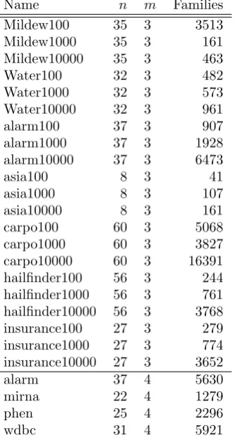
Table 1: Datasets, parent set size limits and family variables used in experiments. nis the number of vari-ables in the dataset, m is the limit on parent set size and ‘Families’ is the number of family variables re-maining after pruning. For the upper set of datasets the number in the dataset’s name records the num-ber of datapoints sampled from the relevant BN. For alarm, mirna, phen and wdbc the number of data-points sampled was 1000, 218, 926 and 569 respec-tively.
collection of BNs in Table 1 all came from Bayesian Network Repository (http://compbio.cs.huji.ac. il/Repository/). Local scores were computed using an unoptimised Python program which meant that it could take as long as an hour to compute local scores for the 3 slowest cases, with the most slow taking a lit-tle over 6 hours. The ‘lower’ 4 datasets were supplied as local scores and are the same as those used in [9].
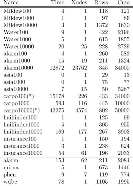
The main results of this paper are contained in the ‘Time’ columns of Tables 2 and 3 which display the time in seconds (rounded to the nearest second, as measured by the UNIX time command, system call time included) to find an optimal BN for all datasets. In Table 2 both 1- and 2-cluster constraints are added. In Table 3 only 1-cluster constraints are used and re-sults for ‘easy’ problems have been omitted in the
[image:6.595.112.279.74.386.2]in-terests of space—they are similar to those found in Table 2. Neither option is consistently better, how-ever using 1-cluster constraints only solves the biggest problem (carpo10000) in ≈ 7.4 hours whereas with both 1- and 2-cluster constraints it takes almost 12 hours. It seems likely that a more careful combination of 1- and 2- cluster constraint cutting planes will be the best option.
For two datasets, carpo100 and carpo10000, it was necessary to impose a time limit of 100 seconds on the sub-IP used to find cutting planes: any solutions found within this limit are added as cutting planes.
On a number of datasets SCIP reached a point at which it could find no further cutting planes but had not found an optimal BN and thus had to resort to branch-and-bound. The ‘Nodes’ column in the tables is the number of nodes in the branch-and-bound tree at the time of solution, so that if Nodes=1 the prob-lem was solved without branching. A branch-and-cut approach was taken: cluster-based cutting planes and Gomory cutting planes are generated not only in the root node of the branch-and-bound tree but at every other node in the tree.
SCIP has a collection of primal heuristicswhich peri-odically search for good solutions. Even if such a so-lution does not turn out to be optimal it can be useful since it may allow pruning of the branch-and-bound tree. In this paper only fast primal heuristics were allowed to run. Typically, the optimal solution (and a number of suboptimal solutions) were found during the running of the simplex algorithm computing a LP solution: if an integral solution is visited in one of the simplex iterations and it turns out to be a valid DAG with a better score than the current incumbent solution, it becomes the new incumbent. This is an instance of SCIP’s simple rounding primal heuristic; in this case there are zero roundings required to pro-duce a solution. In some cases a more sophisticated rounding approach which uses the LP solution, found the optimal BN. Turning off all heuristics modestly speeds up solving for all problems which can be solved in the root, since in that case it is enough to wait for the cutting planes to lead to an LP solution which is entirely integral.
Name Time Nodes Rows Cuts
Mildew100 4 1 118 121
Mildew1000 1 1 97 86
Mildew10000 3 1 1372 1630
Water100 9 1 422 2196
Water1000 5 1 615 1855
Water10000 20 25 228 2729
alarm100 4 1 260 582
alarm1000 15 19 211 1324
alarm10000 12872 23762 345 84000
asia100 0 1 29 13
asia1000 0 1 75 77
asia10000 7 15 50 5287
carpo100(*) 15178 226 433 34000
carpo1000 593 116 445 10000
carpo10000(*) 42275 4574 802 50000
hailfinder100 1 1 125 99
hailfinder1000 5 1 305 955
hailfinder10000 169 177 267 3903
insurance100 1 1 150 194
insurance1000 3 1 238 624
insurance10000 54 61 196 2033
alarm 153 62 211 2084
mirna 5 1 673 1446
phen 9 7 119 774
wdbc 78 1 1105 1995
Table 2: Time taken to find optimal BNs using both 1- and 2-cluster constraints. Problems marked (*) had a 100 second time limit on the sub-IP. For details see the main body of the text.
Name Time Nodes Rows Cuts
Water1000 115 1 604 2121
Water10000 28 1 507 2202
alarm1000 20 28 208 1185
alarm10000 7056 3109 362 6651
asia10000 11 8 49 5788
carpo100(*) 27860 373 644 29000
carpo1000 434 132 589 5451
carpo10000(*) 26774 5205 796 18000 hailfinder10000 934 982 348 5663 insurance10000 61 56 214 1389
alarm 97 7 189 929
phen 12 13 142 559
[image:7.595.80.305.89.402.2]wdbc 68 1 651 1057
Table 3: Time taken to find optimal BNs using only 1-cluster constraints. Problems marked (*) had a 100 second time limit on the sub-IP. For details see the main body of the text.
To test the effectiveness of Gomory cuts, solving was attempted again for each dataset with both 1- and 2-cluster constraints but with Gomory cuts disabled. For all but the largest problems solving was still success-ful and was generally a little quicker. However for big problems disabling Gomory cuts could be disastrous. alarm10000 took 18462 seconds to solve (as opposed to 12872 with Gomory cuts). hailfinder10000, which took only 169 seconds to solve with Gomory cuts had still failed to find an optimal BN after 85075 seconds without them (and had exhausted RAM by this point). With Gomory cuts, the 358−56 = 302 non-redundant cuts generated for hailfinder10000 had reduced the up-per bound on the objective function to−4.970794×10⁵
before SCIP had to resort to branching. Since the opti-mal BN has score−4.976318×10⁵this upper bound is
quite tight allowing for a reasonably fast branch-and-cut search. Without Gomory branch-and-cuts the 502−56 = 446 non-redundant cuts generated had only reduced this upper bound to−4.946169×10⁵. Using Gomory cuts
had allowed for fewer but better cuts. The very largest problems, carpo100 and carpo10000 were not even at-tempted without Gomory cuts.
5.1 How to reproduce these results
Go to:
http://www.cs.york.ac.uk/~jc/research/uai11
6
Ongoing work
The approach described above is the most successful to date but there are a number of elaborations which have been attempted. Although these have yet to ren-der any consistent improvement it is instructive to list them since (1) it may be that some variant will succeed and (2) negative results are of independent interest.
The most obvious idea is to add a reasonably small number ofk-cluster constraints directly into the IP so that they do not have to be found as cutting planes. There is the possibility that SCIP’s pre-processing al-gorithms might be able to simplify the problem using these constraints. In the event, pre-adding k-cluster constraints led to slower solving and increased mem-ory requirements.
gener-ate very many random orders of the BN variables and return the highest-scoring BN consistent with each or-der, ultimately returning the best BN overall. In the second a variable ordering is generated from the cur-rent LP solution with a view to being ‘as consistent as possible’ with it. The best BN for that ordering is then proposed. Both of these approaches are quick, but the BNs found are less useful than those found by rounding (Section 5).
The presented approach makes no use ofMarkov equiv-alence classeswhich partition the BN space into equiv-alent statistical models. BNs in a Markov equivequiv-alent class will have the same score, for any reasonable scor-ing function. Since two BNs are Markov equivalent if they have the same undirected skeleton and set of ‘im-moralities’ (unmarried parents) n2
auxiliary binary line variables were created each indicating the pres-ence/absence of an edge in the undirected skeleton. Since such variables can be defined in terms of fam-ily variables there is no real increase in the number of variables in the IP. Branching priorities were set so that branching could only occur on line variables. The idea here is that branching divides Markov equiv-alence classes rather than just BNs. In most cases this approach slowed down solving but for alarm10000 and alarm solving took only 6526 and 84 seconds re-spectively, which is better than the results reported in Tables 2 and 3.
7
Related work
As previously noted, this work is most closely related to that of Jaakkola et al [9], since the key 1-cluster constraints were introduced in that paper. The main difference is that these constraints are applied here in a conventional manner: as cutting planes in an existing integer programming framework (SCIP). Although, as here, Jaakkola et al add 1-cluster constraints ‘on the fly’ they use a different search approach to find good clusters (actually two search methods are used). When branching they always choose the node with the best LP solution (in the hope that the optimal BN is in that subtree). The variable to branch on is determined by a rule informed by the existence of cluster constraints. Here, in contrast, SCIP’s default approach to branch-and-cut is used.
An empirical comparison is also possible since the same local scores have been used. Jaakkolaet al used a 2.4GHz Dual Core Macbook pro Laptop with 4GB of memory and report solving times of 8 seconds, 7 minutes and 21 minutes for datasets phen, wdbc and alarm respectively. Here these were solved in 9 sec-onds, 1.3 minutes and 2.55 minutes respectively. Note that SCIP does not resort to branching on 2 of the 4
datasets from Jaakkolaet al.
Other much bigger problems have also been solved, al-beit sometimes very slowly. Note that in common with Jaakkolaet al no consideration is given to how ‘close’ the found optimal BNs are to the true data-generating BNs, the focus here is exclusively on the ‘search’ part of a ‘search-and-score’ learning algorithm. This close-ness depends crucially on the score (particularly the choice of Dirichlet priors [11]) as well as, of course, the amount of data.
8
Conclusions and future work
The main finding of this paper is that integer pro-gramming can be used for exact learning of Bayesian networks with quite a large number of variables, the carpo datasets have 60 BN variables—as long as there is a limit on parent set sizes.
In some cases there is a known limit on parent set sizes. For example in the BN representation of a pedi-gree, variables represent individuals and the arrows in the DAG represent real parenthood relationships. Pedigrees are often called ‘family trees’ although the DAG need not be a tree if there has been inbreed-ing. Pedigrees are learnt (or ‘reconstructed’ as it is known in the statistical genetics literature) from DNA marker data. Cowell [5] has applied a dynamic pro-gramming approach to exact pedigree reconstruction whereas Cussens [7] used the IP approach outlined in Section 3
In most other applications the limit on parent set size is artificial. An interesting avenue for future work is to see whether a column generation approach using a variable pricer can be used to overcome this limita-tion. A variable pricer allows the dynamic generation of new variables. Here these would be new family vari-ables. SCIP provides a convenient and effective way of creating variable pricers due to its plugin approach.
equiva-lence class can be ruled out via appropriate constraints and a new search can be started. An advantage of this approach is that there is a guarantee that any yet-to-be-found BNs can have a score no better than those found already. This could be used to provide a bound of the probability mass found so far.
Acknowledgements
Many thanks to Tommi Jaakkola for providing datasets and answering various questions. Thanks to Ricardo Silva for pointing me to Jaakkola et al [9]. The following SCIP developers helped with various as-pects of their framework: Tobias Achterberg, Timo Berthold, Ambros Gleixner, Stefan Heinz, Michael Winkler and Kati Wolter. Particular thanks to Kati Wolter for advice on how to generate extra Gomory cuts. Three anonymous reviewers provided valuable advice on how to improve the original submission.
References
[1] Tobias Achterberg. Constraint Integer Program-ming. PhD thesis, TU Berlin, July 2007.
[2] Tobias Achterberg. SCIP: Solving constraint inte-ger programs. Mathematical Programming Com-putation, 1(1):1–41, July 2009.
[3] David Maxwell Chickering, David Heckerman, and Christopher Meek. Large-sample learning of Bayesian networks is NP-hard. Journal of Ma-chine Learning Research, 20:1287–1330, October 2004.
[4] Thomas H. Cormen, Charles E. Leiserson, and Ronald L. Rivest. Introduction to Algortithms. MIT Press, 1990.
[5] Robert G. Cowell. Efficient maximum likelihood pedigree reconstruction. Theoretical Popluation Biology, 76(4):285–291, December 2009.
[6] James Cussens. Bayesian network learning by compiling to weighted MAX-SAT. In Proceed-ings of the 24th Conference on Uncertainty in Ar-tificial Intelligence (UAI 2008), pages 105–112, Helsinki, 2008. AUAI Press.
[7] James Cussens. Maximum likelihood pedigree re-construction using integer programming. In Pro-ceedings of the Workshop on Constraint Based Methods for Bioinformatics (WCB-10), Edin-burgh, July 2010.
[8] C de Campos, Z Zeng, and Q Ji. Structure learn-ing of Bayesian networks uslearn-ing constraints. In Proc. of the 26th International Conference on Ma-chine Learning, 2009.
[9] Tommi Jaakkola, David Sontag, Amir Globerson, and Marina Meila. Learning Bayesian network structure using LP relaxations. InProceedings of 13th International Conference on Artificial Intel-ligence and Statistics (AISTATS 2010), volume 9, pages 358–365, 2010. Journal of Machine Learn-ing Research Workshop and Conference Proceed-ings.
[10] Mikko Koivisto and Kismat Sood. Exact Bayesian structure discovery in Bayesian networks.Journal of Machine Learning Research, 5:549–573, 2004.
[11] T. Silander, P. Kontkanen, and P. Myllym¨aki. On sensitivity of the MAP Bayesian network struc-ture to the equivalent sample size parameter. In R. Parr and L. van der Gaag, editors, Proceed-ings of the The 23rd Conference on Uncertainty in Artificial Intelligence (UAI-2007), pages 360– 367. AUAI Press, 2007.
[12] Tomi Silander and Petri Myllym¨aki. A simple ap-proach for finding the globally optimal Bayesian network structure. In UAI, 2006.