This is a repository copy of Modelling route choice behaviour in a tolled road network with
a time surplus maximisation bi-objective user equilibrium model
.
White Rose Research Online URL for this paper:
http://eprints.whiterose.ac.uk/79927/
Article:
Wang, JYT and Ehrgott, M (2013) Modelling route choice behaviour in a tolled road
network with a time surplus maximisation bi-objective user equilibrium model.
Transportation Research Part B: Methodological, 57. 342 - 360. ISSN 0191-2615
https://doi.org/10.1016/j.trb.2013.05.011
Reuse
Unless indicated otherwise, fulltext items are protected by copyright with all rights reserved. The copyright exception in section 29 of the Copyright, Designs and Patents Act 1988 allows the making of a single copy solely for the purpose of non-commercial research or private study within the limits of fair dealing. The publisher or other rights-holder may allow further reproduction and re-use of this version - refer to the White Rose Research Online record for this item. Where records identify the publisher as the copyright holder, users can verify any specific terms of use on the publisher’s website.
Takedown
If you consider content in White Rose Research Online to be in breach of UK law, please notify us by
Modelling route choice behaviour in a tolled road network
with a time surplus maximisation bi-objective user
equilibrium model
Judith Y.T. Wanga,b,∗, Matthias Ehrgotta,c
aDepartment of Engineering Science, The University of Auckland, Private Bag 92019, Auckland 1142, New Zealand
bSchool of Civil Engineering & Institute for Transport Studies, University of Leeds, Woodhouse Lane, Leeds LS2 9JT, UK
c
Department of Management Science, Lancaster University Management School, Bailrigg, Lancaster LA1 4YX, UK
Abstract
In this paper, we propose a novel approach to model route choice behaviour in a
tolled road network with a bi-objective approach, assuming that all users have two
objectives: (1) minimise travel time; and (2) minimise toll cost. We assume
fur-ther that users have different preferences in the sense that for any given path with
a specific toll, there is a limit on the time that an individual would be willing to
spend. Different users can have different preferences represented by this
indiffer-ence curve between toll and time. Time surplus is defined as the maximum time
minus the actual time. Given a set of paths, the one with the highest (or least
neg-ative) time surplus will be the preferred path for the individual. This will result
in a objective equilibrium solution satisfying the time surplus maximisation
bi-objective user equilibrium (TSmaxBUE) condition. That is, for each O-D pair, all
individuals are travelling on the path with the highest time surplus value among all
the efficient paths between this O-D pair.
∗
Corresponding author. Tel.: +44 113 343 3259 ; Fax: +44 113 343 3265.
Email addresses:[email protected](Judith Y.T. Wang),
We show that the TSmaxBUE condition is a proper generalisation of user
equi-librium with generalised cost function, and that it is equivalent to bi-objective user
equilibrium. We also present a multi-user class version of the TSmaxBUE
condi-tion and demonstrate our concepts with illustrative examples.
Keywords: Traffic assignment, route choice, equilibrium problem,
multi-objective optimisation
1. Introduction
1
The last stage of a conventional four-stage transport planning model, traffic
2
assignment, is essentially modelling the route choice behaviour of travellers and
3
their interactions. Whether a traffic assignment model can realistically represent
4
travel behaviour is, therefore, dependent on the behavioural assumptions behind
5
the route choice model. In tolling analysis, there are basically two approaches
6
in practice as described in Florian (2006): (1) models based on generalised cost
7
path choice; and (2) models based on explicit choice of tolled facilities. These
8
two approaches follow the principles of the two classic traffic assignment models
9
in the literature, namely, the user equilibrium (UE) model and the stochastic user
10
equilibrium (SUE) model.
11
Wardrop (1952) defineduser equilibriumas:
12
“No user can improve his travel time by unilaterally changing routes.”
13
This is known as Wardrop’s first principle which has two key assumptions:
14
(1) all users have the same objective, i.e. to minimise travel time or generalised
15
cost; and (2) users have perfect knowledge of the network, i.e. they know the travel
16
times that would be encountered on all available routes between their origin and
17
destination. The second assumption is considered to be a strong assumption. Dial
(1971) was the first to introduce a probabilistic assignment concept to address this
19
problem. He proposed a probabilistic multipath traffic assignment model based on
20
the following functional principles:
21
1. The model gives all efficient paths between a given origin and destination a
22
non-zero probability of use, while all inefficient paths have a probability of
23
zero.
24
2. All efficient paths of equal length have an equal probability of use.
25
3. When there are two or more efficient paths of unequal length, the shorter has
26
the higher probability of use.
27
The meaning of ‘efficient’ paths in Dial’s model is defined as a path that does
28
not backtrack, i.e. as it progresses from node to node, it always gets further from
29
the origin and closer to the destination. Every link in an efficient path has its
30
initial node closer to the origin than its final node and its final node closer to the
31
destination than its initial node. In this manner, the set of ‘efficient’ paths can be
32
considered as the reasonable choices. By introducingdiversion curves, Dial (1971)
33
incorporated the logit function into his model which enables the solution to be
34
expressed in explicit form. However, congestion effects have not been considered
35
in this model as link travel time is assumed to be constant.
36
SUE was developed by Daganzo and Sheffi (1977) based on variation of the
37
first assumption of Wardrop’s first principle by considering the objective as
min-38
imising theperceivedcost which is modelled as a stochastic function rather than
39
the static generalised cost function. Daganzo and Sheffi (1977) definedstochastic 40
user equilibriumas:
41
“No user can improve his perceived travel time by unilaterally changing routes”
In order to translate this SUE equilibrium condition into its mathematical
def-43
inition, Daganzo and Sheffi introduced a user’s perceived travel time function on
44
routek,T˜k, which has two components as follows:
45
˜
Tk=Tk+ǫk, (1)
whereTkis the systematic component which is the measured travel time on route
46
k; andǫkis an error term representing the random component which varies from
47
user to user.
48
Hereǫis randomly distributed with a mean value of zero. Thus,
49
ET˜k
=Tk. (2)
Every user then evaluates the travel time on all routes and selects the routekmin
50
with the minimum perceived travel time, i.e.
51
˜
Tkmin≤T˜kfor allk6=kmin. (3)
The mathematical conditions for SUE within this modelling framework are
52
formally defined in Daganzo and Sheffi (1977). The assumption on the distribution
53
of the error term,ǫk, varies. The most commonly used distributions are Gumbell
54
and normal distributions, known as the logit and probit models, respectively. The
55
assumption of the error term following Gumbell/normal distributions is the key
56
linkage of Dial (1971)’s probabilistic model to Discrete Choice Models, which led
57
to further development of SUE traffic assignment models that appeared later in the
58
literature such as Fisk (1980)’s logit-based model and Sheffi and Powell (1982)’s
59
probit model. It is important to note that in order to take congestion effects into
60
consideration, travel time should be flow-dependent. Fisk (1980) was the first to
61
consider the effect of congestion in a stochastic manner, as travel time is considered
62
to be independent of traffic flow in the previous models (Daganzo and Sheffi, 1977;
63
Dial, 1971).
A disadvantage of the probit model is well known as the intensive
computa-65
tional effort requiring Monte Carlo or other numerical techniques (Maher, 1992;
66
Rosa and Maher, 2002). Logit models have their weaknesses but a very
impor-67
tant advantage of having a closed form solution. Thus, the most commonly used
68
stochastic traffic assignment model for toll analysis is a logit-based model as
de-69
scribed in Florian (2006). The key weakness of the most commonly used
logit-70
based model is the validity of the property of independence of irrelevant
alterna-71
tives (IIA), which can be stated as:
72
“Where any two alternatives have a non-zero probability of being chosen, the ratio
73
of one probability over the other is unaffected by the presence or absence of any
74
additional alternative in the choice set (Luce and Suppes, 1965).”
75
When it comes to modelling path choice, the IIA property can be easily
vi-76
olated because of extensive overlapping of possible paths in a choice set for the
77
same origin-destination (OD) pair. Over the last two decades, there were extensive
78
developments in stochastic route choice models trying to address this weakness.
79
Prashker and Bekhor (2004) provide a comprehensive review of the developments.
80
Since the perceived cost function has two components as shown in Equation (1),
81
this problem can be addressed by tackling either the systematic or the error
com-82
ponent. In principle, the technique being used is to make adjustments to these two
83
components such that the resulting solution reflects reality better. Prashker and
84
Bekhor (2004) classified the techniques into three categories: (1) modifications
85
of the basic multinomial logit (MNL) model, such as C-logit and path-size logit
86
(PSL); (2) generalised extreme value (GEV) models, such as paired combinatorial
87
logit (PCL) and cross-nested logit (CNL); and (3) logit kernel (LK) or mixed logit
88
models. The first category adjusts the systematic component while the second and
89
the third adjust the error component.
In this paper, we propose a novel approach to model route choice behaviour
91
in a tolled network. We extend our work in Wang et al. (2010) on bi-objective
92
traffic assignment to incorporate the capability to model the differences between
93
individuals in terms of their willingness to pay. First of all, we assume that all
94
users have two objectives: (1) to minimise travel time; and (2) to minimise toll
95
cost. Users are all rational in the sense that given a choice set, they will only choose
96
one of theefficientpaths. Efficient paths are defined as the set of paths for each
O-97
D pair for which neither time nor travel time can be improved without worsening
98
the other (Wang et al., 2010). According to this definition, at equilibrium, all the
99
used paths between a given O-D pair areefficient. We define bi-objective user 100
equilibrium(BUE) as follows:
101
“Underbi-objective user equilibriumconditions traffic arranges itself in such a
102
way that no individual trip maker can improve either his/her toll or travel time or
103
both without worsening the other objective by unilaterally switching routes.”
104
Dial (1979) is one of the first to introduce multiple objectives in traffic
assign-105
ment. According to BUE, when we consider time and toll cost separately, there is
106
no need to add them up as generalised cost. However, in Dial’s model (Dial, 1979,
107
1996, 1997), a simplification was made by adding time and toll cost in a linear
108
choice function, which is essentially the same as the generalised cost function, but
109
with a probabilistic component by assuming that the value-of-time (VOT) follows
110
a certain probability density function. As discussed in Wang et al. (2010), Dial’s
111
approach might miss out some efficient paths. In Wang et al. (2010); Raith et al.
112
(2013), we developed heuristics to find BUE solutions without missing efficient
113
paths. It is clear that according to the BUE definition, there would be many possible
114
equilibrium solutions rather than one as in conventional static UE. Given there are
115
so many possible equilibrium solutions satisfying the BUE condition, we must
ther develop this model to incorporate the consideration of individual preferences
117
in order to be able to replicate their route choice behaviour more realistically.
118
There is no doubt that route choice behaviour in a tolled road network is
119
stochastic in nature since individuals might not choose the shortest path for all
120
sorts of reasons and the willingness to pay would vary among individuals. As
dis-121
cussed above, probabilistic models such as Dial (1979)’s or the logit-based SUE
122
traffic assignment models such as Fisk (1980)’s all possess some deficiencies. The
123
philosophy behind the proposed model is to overcome these difficulties, including
124
the possibility of missing efficient paths in Dial (1979)’s model and the limitations
125
induced by the IIA property of the logit-based SUE traffic assignment model, by
126
introducing an indifference function which can vary between individuals with no
127
restrictions. As with any models, there are, however, some key assumptions to be
128
made:
129
1. Users are all rational in the sense that they will only choose one of the effi-130
cientpaths.
131
2. Users have differentpreferenceswhich can be represented by an indifference
132
function between toll and time. Users’ behaviour as represented by this
in-133
difference function is rational, i.e. the maximum time that a user is willing
134
to spend will always be shorter for higher toll.
135
3. Preferences among users vary in the sense that their preferred paths can be
136
different, even though they are considering the same choice set.
137
4. Users have perfect knowledge of the network, as in standard user equilibrium
138
models.
139
With this new approach, each individual will only choose from a reasonable
140
choice set and choose according to his/her own preference.
This paper is organised as follows. In Section 2, we review standard user
equi-142
librium for traffic assignment. In Section 3, we introduce bi- and multi-objective
143
user equilibrium and investigate their relationship with single objective user
equi-144
librium. Section 4 is devoted to the description of our new concept of time surplus
145
maximisation bi-objective user equilibrium. We show that this generalises user
146
equilibrium based on generalised cost functions and prove its equivalence to
bi-147
objective user equilibrium. Section 5 provides an illustrative example of the idea,
148
whereas Section 6 extends the idea to multiple user classes, which is then
illus-149
trated in Section 7. Finally, Section 8 discusses the importance of the findings in
150
this paper and Section 9 concludes with an outlook for future research.
151
2. User Equilibrium
152
In this section we introduce equilibrium models of traffic assignment. LetG=
(N, A)denote a (transportation) network, whereN is a set of|N|nodes andA⊂
N×N is a set of|A|arcs or links. Moreover, letZ ⊂N ×N be a set of
origin-destination pairs (O-D pairs) and for allp∈Z, letDpdenote the demand for travel
between the origin and destination of O-D pairp. Equilibrium models attempt to
determine the amount of trafficfaon all linksa∈Aunder some assumptions on
the behaviour of road users. One of these assumptions is that road users choose the
pathk∗between their origin and destination that minimises a cost functionCk:
k∗= argmin{Ck:k∈Kp},
whereKpis the set of all simple paths from the origin of O-D pairpto its
destina-153
tion.
154
To formalise the idea of user equilibrium, letδk
abe an indicator withδka = 1if
155
and only if linkais contained in pathkand 0 otherwise. Thenfa=Pp∈ZPk∈Kp
156
δk
aFk, whereFkis the flow on pathk∈Kp. The costCk(F)of pathkmay depend
on the entire vectorF= (F1, . . . , F|K|)of flows on all pathsk∈K :=∪p∈ZKp.
158
The user equilibrium condition of Wardrop’s first principle states that the cost of all
159
used paths is equal and less than that which would be experienced by a single user
160
on any unused route. It is well known that this principle assumes that all users are
161
the same in that they want to minimise the costCk and that all users have perfect
162
information about the cost function, see e.g. Sheffi (1985).
163
Let Up := mink∈KpCk(F) denote the minimum cost of any path for O-D
164
pairp ∈ Z. Then, following e.g. Florian and Hearn (1995), the user equilibrium
165
condition can be written mathematically as follows: Path flow vector F∗ is an
166
equilibrium flowifF∗ satisfies conditions (4) – (8):
167
Fk∗(Ck(F∗)−Up) = 0 for allk∈Kpand allp∈Z, (4)
Ck(F∗)−Up ≥ 0 for allk∈Kpand allp∈Z, (5)
X
k∈Kp
Fk∗−Dp = 0 for allp∈Z, (6)
Fk∗ ≥ 0 for allk∈K, (7)
Up ≥ 0 for allp∈Z. (8)
Equation (4) states that if flow on pathkis positive then the costCk(F∗)has to
168
be minimal, whereas ifCk(F∗)> Upthen the flow on pathkmust be 0. Equation
169
(5) says that all path costs are greater than or equal to the minimum. Equation
170
(6) guarantees that demand is satisfied, whereas equations (7) and (8) postulate
171
non-negativity of flow and cost. For future use, let us introduce
172
Ω :={F:Fsatisfies (6)−(7)} (9)
to denote the set of all feasible path flow vectorsF.
173
Existence of a solution of the network equilibrium model (4) – (8) is guaranteed
174
if the path cost functionsCk(F)are all positive and continuous. In addition, for
uniqueness of the solution,Ck(F)must be strictly monotone (Florian and Hearn,
176
1995).
177
The most important cost function is travel time. In this paper we use the
com-178
mon Bureau of Public Roads (1964) function to model the relation between travel
179
time and traffic flow on any linka∈A, i.e.
180
ta(fa) =t0a "
1 +α
fa
Ca
β#
, (10)
wheret0
ais the free-flow travel time on linka,Cais the practical capacity of linka
181
in vehicles per time unit, andα, βare function parameters. If the cost functionCk
182
considered in (4) – (8) is path travel time, then
183
Ck(F) =Tk(F) := X
a∈k
ta(fa) (11)
for allk∈K.
184
Conventional traffic assignment assumes that path cost functions Ck(F) are
185
additive and separable. Additivity means thatCk(F) =Pa∈kca(f)can be written
186
as the sum of link cost functionsca(f), wheref := (f1, . . . , f|A|)is the link flow
187
vector. Separability means that the link cost functions ca(f) depend only on the
188
flowfaon linka, i.e.ca(f) =ca(fa).
189
Under these assumptions it is well known (Beckmann et al., 1956) that the
190
network equilibrium model (4) – (8) can be reformulated as a mathematical
pro-191
gramme
192
minX
a∈A Z fa
0
ca(x)dx, (12)
subject to X
k∈Kp
Fk = Dp for allp∈Z, (13)
Fk ≥ 0 for allk∈K, (14)
fa− X
p∈Z X
k∈Kp
Conventional traffic assignment based on travel time can, therefore, be solved
193
by algorithms for optimising a convex function over a polyhedron. The first
algo-194
rithm used for traffic assignment is the Frank-Wolfe algorithm (Frank and Wolfe,
195
1956) but many others such as path equilibration (Dafermos and Sparrow, 1969),
196
gradient projection (Jayakrishnan et al., 1994) and projected gradient (Florian et al.,
197
2009) methods have been proposed.
198
Many researchers have suggested more general cost functions than travel time,
199
see e.g. Chen et al. (2010); Larsson et al. (2002). Most often Ca(F) takes the
200
form of ageneralised cost functionthat incorporates a linear combination of travel
201
time and a monetary component (Dial, 1996; Leurent, 1993). A generalised cost
202
function is of the form
203
Ck(F) =Mk(F) +αTk(F), (16)
whereMk(F)is the monetary cost associated with pathk. This may be composed
204
of different factors such as toll cost and vehicle operating costs. In addition, α
205
is a value of time, i.e. it converts the travel time Tk(F) into a monetary value.
206
To solve traffic assignment problems with generalised cost function (16), one can
207
apply the same algorithms as for conventional traffic assignment, depending on the
208
properties of functionMk(F). We note, however, that ifCk(F)is not additive, it
209
is necessary to calculate shortest paths based on non-additive costs (Gabriel and
210
Bernstein, 1997), a research topic in its own right.
211
3. Bi-Objective User Equilibrium
212
The generalised cost function (16) combines a monetary component and travel
213
time into a single function via value of timeα. It is reasonable to assume that not
214
all users will have the same value of time, so that a user will choose the route that
215
minimises the generalised cost (16) with a user specific value of time. Dial (1979)
realised this and interpreted the problem as bi-objective problem: Users would
217
be wanting to minimise both travel time and monetary cost. He observed that at
218
equilibrium, all used path will be efficient.
219
Definition 1. LetF∈Ωbe a feasible flow andMk(F)andTk(F)be the monetary
220
and time components of the cost of pathkfor allk∈Kp.
221
1. Pathkisefficient, if there is no pathk′ ∈Kp such thatMk′(F) ≤ Mk(F) 222
andTk′(F)≤Tk(F)with at least one inequality being strict. 223
2. IfMk′(F)≤Mk(F)andTk′(F)≤Tk(F)with at least one strict inequality 224
then pathk′dominatespathkand cost vector(T
k′(F), Mk′(F))dominates 225
(Tk(F, Mk(F)).
226
Dial (1979) describes this idea and an algorithm to find the efficient paths
227
which makes use of the generalised cost function (16) with flow independent
ob-228
jectives. Leurent (1993) applies the idea in traffic assignment and designs an
algo-229
rithm to compute the equilibrium in a tolled road network with toll cost and time
230
as the objectives, where only time is flow dependent. As in Dial (1979), Leurent
231
(1993) assumes that users make their route choice decisions based on a generalised
232
cost function and a continuous value of time distribution is considered. Dial (1996,
233
1997) further develops his idea of 1979 into more efficient algorithms to find the
234
efficient paths and to solve the bi-objective equilibrium problem in which both
235
criteria can be flow dependent.
236
As we have demonstrated in Wang et al. (2010), and as the example in Section
237
5 shows, the procedures of Dial (1997) and Leurent (1993) will only compute
238
equilibrium flows that allow positive flows on a subset of all efficient paths, namely
239
those that are shortest path with respect to the generalised cost function (16) for
240
some positive value ofα. Since all efficient paths can be rational route choices,
241
the work of Leurent and Dial appears to be limited by the use of the functional
form (16) and its underlying assumption of an additive utility function. Removing
243
this form and allowing for more than two objectives one arrives at the definition of
244
multi-objective user equilibrium.
245
Definition 2. LetG= (N, A)be a network,Z ⊂N×N be a set of O-D pairs and
246
for allp∈Z, letDpbe the demand of O-D pairp. LetCk(i)(F), i= 1, . . . , rber
247
cost functions of pathkand letCk(F)denote the cost vector of pathk. Feasible
248
flowF∗ ∈Ωis amulti-objective equilibrium flow, if wheneverCk(F∗)dominates
249
Ck′(F∗)fork, k′ ∈Kp for anyp∈ZthenFk′ = 0. 250
Definition 2 is the multi-objective generalisation of the equilibrium conditions
251
(4) – (8). Only efficient paths can carry positive flow, whereas dominated paths
252
have zero flow. Ifr= 2, we talk about bi-objective equilibrium flow. In the case of
253
r = 1, Definition 2 reduces to the standard equilibrium condition. In Wang et al.
254
(2010) we have shown that even for the case r = 2 and even if both objectives
255
are separable and additive, and one of the objectives does not depend on flow, the
256
multi-objective user equilibrium condition is not equivalent to a multi-objective
257
version of Beckmann’s formulation (12) – (15). A discussion of the similarities
258
and differences of multi-objective equilibrium, optimisation, and vector inequality
259
problems is provided in Raith and Ehrgott (2011).
260
Moreover, there are usually infinitely many flow vectorsF∈Ωthat satisfy the
261
condition of Definition 2.
262
The concept of multi-objective user equilibrium therefore provides a general
263
framework for investigating equilibrium flows in the presence of multiple
objec-264
tives. Under the assumption that the objectives considered are those relevant for
265
users’ route choice, one of these multi-objective equilibrium solutions will be
re-266
alised in practice. Which one that is will depend on user preferences and trade-offs
267
between the objectives. The simplest model of user preferences is the additive form
as shown in (16). In this paper, we develop a more general model. But before we
269
proceed to this model, we formally show that the multi-objective user equilibrium
270
is a proper generalisation of the single objective model with generalised cost (16).
271
Proposition 1. LetG= (N, A)be a network,Z ⊂N ×N be a set of O-D pairs
272
and for allp ∈ Z, let Dp be the demand of O-D pairp. Letr = 2. LetF∗ be
273
an equilibrium flow with respect to generalised cost functionC(F) :=C(1)(F) +
274
αC(2)(F)for some positive numberα. ThenF∗is also a bi-objective equilibrium
275
flow for objective functionsC(1)(F)andC(2)(F).
276
PROOF. Assume the contrary. Then there exists ap∈Zand two pathsk, k′ ∈Kp
withFk, Fk′ > 0 such thatCk′(F) dominates Ck(F). Then, because α > 0, it
holds that
Ck(1)′ (F) +αC
(2)
k′ (F)< C
(1)
k (F) +αC (2) k (F),
contradicting the equilibrium condition for the generalised cost function.
277
In fact, with the same argument, it is possible to show a more general result.
278
Theorem 1. LetG= (N, A)be a network,Z⊂N×N be a set of O-D pairs and
279
for allp ∈ Z, letDpbe the demand of O-D pairp. Letg : Rr → Rbe a strictly
280
increasing function in allrarguments. LetF∗ be an equilibrium flow with respect
281
to generalised cost functionC(F) :=g(C(F)). ThenF∗is also a multi-objective
282
equilibrium flow for objective functionsC(1)(F), . . . , C(r)(F).
283
In Section 4, we will address the case of equilibrium problems with r = 2
284
objectives, where Ck(1)(F) = Tk(F) and C(2)
k (F) = Mk(F) and the monetary
285
objective consists of exogenously defined tolls. We investigate bi-objective user
286
equilibrium for these functions and a specific nonlinear function to combine them.
4. The Time Surplus Maximisation Model
288
In this section, we develop the time surplus maximisation equilibrium model
289
as a new model for route choice behaviour in tolled road networks. From now on,
290
we will consider two objective functions, namely, travel timeCk(1)(F) =Tk(f) =
291
P
a∈kta(xa), where ta(xa) is the travel time function (10) and toll Ck(2)(F) =
292
Mk(f) = τk = Pa∈kτa, with exogenously defined link tolls τa. Hence, both
293
path objectives (travel time and toll) are additive, link travel time and link toll are
294
separable, and link toll does not depend on flow.
295
4.1. The Indifference Function 296
To start with, we assume that given an O-D pairp, each user has an indifference
297
function between toll and time. For any given pathkwith a specific toll, there is a
298
limit on the time that a user would be willing to spend. We model this indifference
299
function as a functionTmax
p :R→Rthat is strictly decreasing, i.e.Tpmax(τk1) <
300
Tpmax(τk2) ifτk1 > τk2. This takes into account that users would expect to spend
301
less time in traffic if they need to pay a higher toll. An example of an indifference
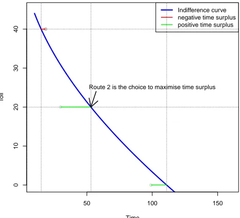
302
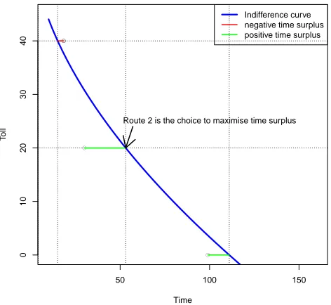
curve is shown in Figure 1.
303
Time surplus is defined as the time that the user would be willing to spend
304
minus the actual travel time. The time surplus for a path can be positive or
nega-305
tive. Given a choice set of paths, the one with the highest time surplus will be the
306
preferred path for the individual.
307
A positivetime surplus value can be viewed as virtually the pleasure for an
308
individual obtained from choosing this path, whereas anegativetime surplus value
309
can represent an unfavourable choice and the magnitude of this path being disliked.
310
One would expect that given a set of efficient paths with both positive and negative
311
time surplus values, only the one with positive time surplus values will be
consid-312
ered. For example, an individual with an indifference curve as shown in Figure 1
50 100 150
0
10
20
30
40
Time
T
oll
Indifference curve negative time surplus positive time surplus
●
●
●
[image:17.612.182.418.156.373.2]Route 2 is the choice to maximise time surplus
Figure 1: An indifference curve between time and toll.
will only consider the two paths that have positive time surplus, i.e the ones with
314
τk = 20 and the one withτk = 0. Among these two, the one with τk = 20 is
315
considered more attractive as the time surplus value is higher.
316
There is, however, the possibility that all the efficient paths have negative time
317
surplus values for a user who is both unwilling to pay and to spend time. In that
318
case, we will have to assume either this user would not travel at all or will have to
319
make a choice based on the negative values. In this paper, we assume that the total
320
demand is inelastic and hence the user will choose the path with the least negative
321
time surplus value.
4.2. The Time Surplus Maximisation BUE Condition 323
Given the indifference curvesTpmax for allp ∈ Z, we define time surplus for
324
pathk∈Kpas
325
T Sk(F) :=Tpmax(τk)−Tk(f) =Tpmax X
a∈k
τa !
−X
a∈k
ta(fa). (17)
.
326
We note that functionT Sk(F)is not additive becauseTpmax(τ)is only defined
327
for OD pairpbut neither for paths nor for links and, therefore, cannot be written as
328
the sum of link indifference functions. Moreover,Tmax
P may be non-linear. Hence,
329
all equilibrium models using this function will be path based. Assuming that users
330
choose the pathk∗with maximum time surplus, i.e.
331
k∗ = argmin{T Sk(F) :k∈Kp}, (18)
we can now formulate the Time Surplus Maximisation Bi-objective User
Equilib-332
rium (TSmaxBUE) condition.
333
Definition 3. Path flow vectorF∗is called atime surplus maximisation
bi-objecti-334
ve user equilibriumflow ifFk > 0⇒ T Skmax(F∗) ≥ T Skmax′ (F∗)for allk, k′ ∈ 335
Kp, or equivalently, ifTkmax(F)> T Skmax′ (F)⇒Fk′ = 0. 336
In words, the TSmaxBUE condition states that
337
“Under theTime Surplus Maximisation equilibriumcondition traffic arranges
338
itself in such a way that no individual trip maker can improve his/her time surplus
339
by unilaterally switching routes,”
340
or alternatively
341
“Under theTime Surplus Maximisation equilibrium conditionall individuals are
342
travelling on the path with the highest time surplus value among all the efficient
343
paths between each O-D pair.”
Next, we show that the TSmaxBUE model is a special case of the general
multi-345
objective user equilibrium model of Definition 2, but that it is more general than
346
the single objective user equilibrium with generalised cost function (16) based on
347
value of time.
348
Theorem 2. LetG = (N, A)be a network, Z ⊂ N ×N be a set of O-D pairs
349
with demandDp >0for allp ∈Z. Letτadenote the toll of linkaandta(fa)be
350
the travel time function of linka. Assume thatF∗is a TSmaxBUE flow. ThenF∗is
351
also a bi-objective equilibrium flow with respect to the objectivesC(1)(F) =Tk(f)
352
andC(2)(F) =τ k.
353
PROOF. We have to show that all paths k with F∗
k > 0 are efficient paths with
354
respect toC(1)andC(2). So assume thatF∗is such that there is somep∈Z and
355
k, k′ ∈ Kp such thatC(Fk) dominatesC(F)k∗′. That is,Tk(Fk∗) ≤Tk′(F∗
k′)and 356
τk≤τk′ with one strict inequality. 357
Then we have
358
T Sk(Fk∗) =Tpmax(τk)−Tk(Fk∗)> Tkmax′ (τk′)−Tk′(Fk∗′) =T Sk′(Fk′) (19)
because of the dominance and becauseT Smax is a strictly decreasing function.
359
Clearly (19) contradicts the assumption thatF∗ is a TSmaxBUE flow.
360
It is even possible to prove the converse of Theorem 2.
361
Theorem 3. LetG= (N, A)be a network,Z ⊂N×N be a set of O-D pairs with
362
demandDp > 0for allp ∈ Z. Letτadenote the toll of linkaandta(fa)be the
363
travel time function of linka. Assume that F∗ is a bi-objective equilibrium flow,
364
with respect to objectivesC(1)(F)andC(2)(F)as in Theorem 2. Then there exists
365
an indifference functionTmaxsuch thatF∗is also a TSmaxBUE flow.
PROOF. Let F∗ be a bi-objective equilibrium flow. According to Definition 2,
367
all paths with positive flow are efficient. LetK∗
p be the set of all efficient paths
368
for O-D pair p ∈ Z. Then for paths k, k′ ∈ Kp∗ we have thatτk > τk′ implies 369
Tk(Fk) < Tk′(Fk′) and can therefore order the paths in Kp∗ = {1, . . .|Kp∗|}in 370
such a way thatτk> τk′ andTk< Tk′ if and only ifk > k′. 371
In case there is no efficient path with τk = 0 or τk = max{τk : k ∈ K}
372
we add (one of) the points (τ0 = 0, T0 = max{Tk(Dp) : k ∈ K, p ∈ Z})
373
and(τ|K∗
p|+1 = max{τk : k ∈ K}, T|Kp∗|+1 = 0)to the sequence (τk, Tk). We
374
defineTmax(τ) as the uniquely determined piecewise linear function through the
375
points(τk, Tk), k = 0, . . .|Kp∗|+ 1. ClearlyTmax(τ) is strictly decreasing and
376
non-negative.
377
Now observe that for F∗ we have that T Sk(F∗) = 0for all efficient paths
378
k ∈ Kp∗. It remains to show that there does not exist a path with positive time
379
surplus. To see this, assume thatl ∈ Kp is such a path. T Sl(F∗) > 0implies
380
thatTl(Fl∗) < T Smax(τl). Then either (τl, Tl(Fl∗)) < (τk, Tk(Fk∗)) for some
381
k ∈ Kp∗, contradicting the definition of Kp∗ or there are k1, k2 ∈ Kp∗ such that
382
τk1 < τl < τk2 andTk1(F ∗
k1) > Tl(Fl∗)> Tk2(F ∗
k2). In this case, pathldoes not
383
dominate nor is it dominated by any pathkinKp∗. Hence pathlis itself efficient,
384
therefore used in the definition ofTmax, which impliesT Sl= 0.
385
Theorems 2 and 3 imply that the time surplus maximisation equilibrium
con-386
cept is equivalent to the bi-objective user equilibrium, although, of course, the
387
functionT Smaxis in general not known beforehand. We notice that this function
388
is piecewise linear, non-negative and continuous, but in general neither convex nor
389
concave. Concavitiy/convexity of the indifference curveT Smax indicates
willing-390
ness/reluctance to pay, so that TSmaxBUE equilibrium flows with concave/convex
391
indifference curves will form a subset of all bi-objective equilibrium flows that is
more realistic than arbitrary decreasing indifference curves.
393
The next result shows that every equilibrium flow with respect to generalised
394
cost functionC(F) =τk+αTk(Fk), whereα >0is a positive constant, is also a
395
TSmaxBUE flow.
396
Theorem 4. LetG = (N, A)be a network, Z ⊂ N ×N be a set of O-D pairs
397
with demandDp > 0for allp ∈ Z. Let τa denote the toll of linkaandta(fa)
398
be the travel time function of linka. Assume thatF∗ is an equilibrium flow with
399
respect to the generalised cost objectiveC(F) = τk+αTk(f). Then there exists
400
an indifference curveTmaxsuch thatF∗is also a TSmaxBUE flow.
401
PROOF. LetF∗ be an equilibrium flow with respect toCand for allp∈Z define
402
Tmax
p (τ) := a0 − α1τ for some a0 > 0, e.g a0 = max{Tk(Dp) : k ∈ Kp}.
403
We need to show that for any pair of paths kandk′, with time surplus T Sk(F)
404
defined using the just defined functionsTmax
p (τ),T Sk(Fk)> T Sk′(Fk′), implies 405
thatFk′ = 0. 406
T Sk(Fk) > T Sk′(Fk′) ⇔
a0− 1
ατk−Tk(Fk) > a0−
1
ατk′−Tk′(Fk′) ⇔
1
ατk′ +Tk′(Fk′) >
1
ατk+Tk(Fk) ⇔ τk′+αTk′(Fk′) > τk+αTk(Fk) ⇔
C(Fk′) > C(Fk)
Hence, the equilibrium condition for generalised cost functionCimplies thatFk′ = 407
0.
408
The proof of Theorem 4 reveals that any generalised cost equilibrium flow is
409
a special case of a TSmaxBUE flow, with the choice of a linear indifference curve
410
Tmax. Notice that only the slope 1/αof this curve is important, but not its axis
intercepta0. In the example of Section 5, we will see that the converse of Theorem
412
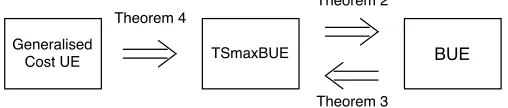
4 does not hold. We can therefore summarise the relationships between generalised
413
cost equilibrium, time surplus maximisation equilibrium and bi-objective
equilib-414
rium in Figure 2.
415
TSmaxBUE BUE
Generalised Cost UE
Theorem 2
[image:22.612.179.433.220.274.2]Theorem 3 Theorem 4
Figure 2: The relationship between equilibrium concepts discussed in this paper.
The proof of Theorem 2 shows that the time surplus of a dominated path is
416
never better than that of any efficient path dominating it, we only includeefficient 417
paths in the choice set which gives us a reasonable choice set. We also note that the
418
time surplus maximisation BUE model basically follows similar functional
princi-419
ples as outlined in Dial (1971).
420
1. Traffic will only be assigned toefficientpaths. Note that we defineefficient 421
paths differently but basically the meaning of our definition also identifies
422
the set of reasonable choices.
423
2. All dominated (inefficient) paths will have zero probability of use.
424
3. If there are two or more efficient paths, the one with the highest time surplus
425
will be chosen.
426
We believe that single objective equilibrium models based on generalised cost
427
functions of the form (16) are restrictive, because they essentially imply, as
Theo-428
rem 4 shows, a linear indifference curve between toll and time. Moreover, (Dial,
429
1997) and (Leurent, 1993) in fact violate the first functional principle above,
be-430
cause some efficient paths in the sense of Definition 1 will always have zero flow.
It is more realistic to assume that there will be users who are willing to pay to
en-432
sure short travel times, whereas others may be reluctant to pay any tolls, and would
433
accept high travel times in order to avoid tolls. The latter would have convex
indif-434
ference curves, while the former users’ indifference curves will be concave. Hence,
435
the variability between individuals in terms of willingness to pay is modelled by
436
the indifference function which leads to their differences in behaviour. We can now
437
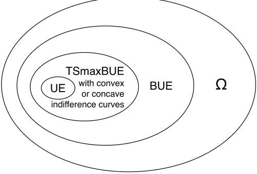
classify the various types of equilibrium flow as in Figure 3. Generalised user
equi-438
librium flows with cost function (16) are TSmaxBUE equilibrium flows with linear
439
indifference curves. More general TSmaxBUE equilibrium flows are generated by
440
convex or concave indifference curves, whereas all bi-objective user equilibrium
441
flows are TSmaxBUE equilibrium flows with arbitrary strictly decreasing
indif-442
ference curves. The proof of Theorem 4 shows that such a curve may be neither
443
convex nor concave.
444
Ω
BUE TSmaxBUE
with convex or concave indifference curves
[image:23.612.180.431.401.571.2]UE
Figure 3: Several classes of equilibrium flows.
We introduce the TSmaxBUE concept with multiple user classes in Section 6,
445
but first, we briefly address solving the TSmaxBUE traffic assignment problem and
present a small illustrative example.
447
In order to be able to solve the TSmaxBUE problem, we use the framework of
448
ageneralised time functionas introduced in Larsson et al. (2002). Larsson et al.
449
(2002) consider time based traffic equilibrium, where users minimise travel time
450
Tkand monetary costτkvia a a generalised time function
451
θk=Tk+g(τk), (20)
whereg : R → R is a nonlinear function, called thetime equivalent of money.
452
Larsson et al. (2002) showed that the equilibrium problem with generalised time
453
(20) is equivalent to an optimisation problem.
454
We introduce the following functiong:R→R:
455
g(x) =h(0)−h(x), (21)
whereh :R → Ris a strictly decreasing function onR+0. Clearly,gis a strictly
456
increasing function ofxonR+0. We substituteTmaxforhand define the path cost
457
function
458
Ck(F) := X
a∈k
ta(fa) +g(τk) = X
a∈k
ta(fa) +Tmax(0)−Tmax(τk). (22)
We observe that because Tmax is a strictly decreasing function of τk,
max-459
imising time surplus is equivalent to minimisingCk. Moreover,Ck(F)is positive
460
becauseTmax(τ) > 0for anyτ ≥0 and because travel times are positive. Path
461
cost functionCk(F
k)in equation (22) is therefore a generalised time function of
462
form (20), and we can apply the results of Larsson et al. (2002) and formulate
463
the time surplus maximisation equilibrium problem as a single objective
equilib-464
rium problem with generalised time function (22). Applying the results of Larsson
465
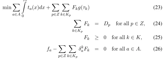
et al. (2002), it follows that this equilibrium problem is equivalent to the
optimisa-466
tion problem (23) – (26), which under our assumptions satisfies the conditions for
unique link flow solutions in Larsson et al. (2002).
468
minX
a∈A fa
Z
0
ta(x)dx+ X
p∈Z X
k∈Kp
Fkg(τk) (23)
X
k∈Kp
Fk = Dp for allp∈Z, (24)
Fk ≥ 0 for allk∈K, (25)
fa− X
p∈Z X
k∈Kp
δkaFk = 0 for alla∈A. (26)
In Section 5, we provide an example illustrating the time surplus maximisation
469
BUE concept.
470
5. A Four Node Example
471
5.1. Network Specification 472
Now we consider a four node network as shown in Figure 4 with link
charac-473
teristics as shown in Table 1.
r
a
b
s
1
2 3
4
5 6
7
8
Tolled links
[image:25.612.154.486.161.281.2]Toll-free links
Figure 4: A four node network.
Table 1: Link characteristics of the four node network.
Link Type Distance Free-flow travel time Toll Capacity
(km) (mins) ($) (veh/hr)
1 Expressway 30 18.0 20 3600
2 Highway 30 22.5 15 3600
3 Arterial 10 12.0 1 1800
4 Arterial 20 24.0 0 1800
5 Arterial 2 2.4 0 1800
6 Arterial 5 6.0 0 1800
7 Arterial 20 24.0 0 1800
8 Arterial 10 12.0 1 1800
The single O-D pair is(r, s)and there are only six feasible routes in this
net-475
work. The routes and their characteristics are listed in Table 2. Note that Route1
476
and Route2are the direct routes, with Route1being the fastest with the highest toll
477
while Route6is the only toll-free route and the slowest. The total demand fromrto
478
sis fixed at 10,000 vehicles per hour which is just a little bit lower than the network
479
corridor capacity of 10,800 vehicles per hour. In order to define the indifference
480
curve, we only need to specify the values ofT Smax(τ
k)for τk = 0,1,2,15,20.
481
These values are shown in the last column of Table 2.
482
The solution F∗ shown in Table 3 is a TSmaxBUE solution. The values of
483
travel time and toll for the four routes with nonzero flow are illustrated in Figure 5.
484
As Theorem 2 states, all routes with positive flow are efficient. Toll-free Route 6
485
is also efficient, but has zero flow because its time surplus, even at free-flow travel
486
time is negative and less than the equilibrium value. Note that Routes 3 and 4 have
Table 2: Route characteristics of the four node network.
Route Path Length Free-flow Travel Time Toll Max Time
1 1 30 18.0 20 25
2 2 30 22.5 15 40
3 3−7 30 36.0 1 50
4 4−8 30 36.0 1 50
5 3−5−8 22 26.4 2 49
6 4−6−7 45 54.0 0 51
identical toll, travel time, and flow and, therefore, show as a single dot in Figure 5.
488
Table 3: Time surplus maximisation BUE solution.
Route Flow Travel time Time Surplus
1 2384.6 18.52 6.48
2 4839.2 33.52 6.48
3 202.9 43.52 6.48
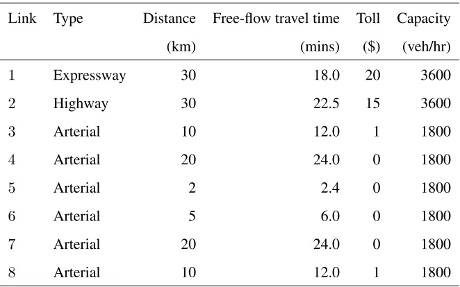
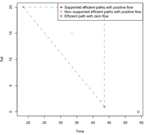
4 202.9 43.52 6.48
5 2370.4 42.52 6.48
6 0.0 54.00 -3.00
We also notice that two of the efficient routes are not optimal for generalised
489
cost (16) for any positive value of time. Hence, this example demonstrates that
490
there are TSmaxBUE flows that are not equilibrium flows for generalised cost
func-491
tions (16), even if a continuous distribution of value of time such as suggested in
492
Dial (1997) is considered. Together with Theorem 4, this means that the time
[image:27.612.201.411.391.534.2]surplus maximisation bi-objective user equilibrium is indeed more general than
494
generalised cost user equilibrium.
495
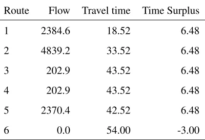
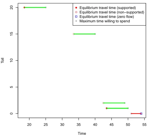
Figure 6 shows in addition to time and toll values the time surplus for each
496
route. This is of course equal for each used route and larger than the (negative)
497
time surplus of unused Route 6.
498
●
● ●
20 25 30 35 40 45 50 55
0
5
10
15
20
Time
T
oll
●
● ●
●
[image:28.612.181.419.261.482.2]Supported efficient paths with positive flow Non−supported efficient paths with positive flow Efficient path with zero flow
Figure 5: Efficient paths do not all optimise generalised cost.
6. Time Surplus Maximisation User Equilibrium with Multiple User Classes
499
In Section 4.2, we indicated that the concept of indifference curve that underlies
500
the time surplus maximisation bi-objective user equilibrium lends itself to
multi-501
user class traffic assignment. The shape of the indifference curve models users’
502
attitude towards tolls in terms of willingness to pay. Users who are unwilling to
●
● ●
20 25 30 35 40 45 50 55
0
5
10
15
20
Time
T
oll
●
●
●
●
● ● ●
●
● ●
●
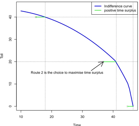
[image:29.612.180.419.278.496.2]Equilibrium travel time (supported) Equilibrium travel time (non−supported) Equilibrium travel time (zero flow) Maximum time willing to spend
pay tolls would accept higher maximum travel times at zero tolls to avoid the tolls.
504
The shape of their indifference curve would be convex, as in Figure 7, whereas
505
users with a strong preference for short travel time would accept any toll in order
506
to ensure short travel times. Their indifference curve would be concave as in Figure
507
8.
508
50 100 150
0
10
20
30
40
Time
T
oll
Indifference curve negative time surplus positive time surplus
●
●
●
[image:30.612.183.417.261.474.2]Route 2 is the choice to maximise time surplus
Figure 7: A convex indifference curve.
The limiting case for users who are reluctant to pay (whose indifference curve
509
is convex) is a quasi-convex function defined as in Equation (27)
510
Tpmax(τ) :=
0 if 0< τ ≤max{τk:k∈Kp}
max{Tk(Dp) :k∈Kp} ifτ = 0,
(27)
whereas the limiting case for a user insensitive to paying tolls (with a concave
10 20 30 40
0
10
20
30
40
Time
T
oll
Indifference curve positive time surplus
●
●
●
[image:31.612.181.418.280.495.2]Route 2 is the choice to maximise time surplus
indifference curve) would be the quasi-concave function as in Equation (28)
512
Tmax p (τ) :=
max{Tk(Dp) :k∈Kp} if 0≤τ <max{τk :k∈Kp}
0 ifτ = max{τk :k∈Kp}.
(28)
Notice that neitherTmax
p norTpmax are strictly decreasing and are, therefore,
513
excluded from being used in the definition of indifference curves in Section 4.1 and
514
the time surplus function (17).
515
To extend Definition 3 to the case of multiple user classes, we let M be the
516
finite set of user classes and denote byDpm the demand for travel for O-D pair
517
p∈ Z and user classm, for allm ∈ M andp ∈Z. Tmax
pm (τ)andT Skm(F)are,
518
respectively, the indifference curve for user classm on origin-destination pairp
519
and the time surplus function of user classmon pathk∈Kp. Moreover, we index
520
path flows by user class, i.e.Fkmdenotes the flow on pathkfor user classm. The
521
set of feasible flows for traffic assignment with multiple user classes is defined as
522
ΩM :=
F∈R|K|·|M|: X
k∈Kp
Fkm =Dpmfor allp∈Z andm∈M
. (29)
Definition 4. Path flow vectorF∗ ∈ΩM is called aTSmaxBUE flow with multiple
523
user classesif for allm ∈M it holds thatFkm >0⇒T Skm(F∗) ≥T Sk′m(F∗) 524
for allk, k′∈K
p, or equivalently, ifTkm(F∗)> T Sk′m(F∗)⇒Fk′m = 0. 525
To find a solution of the time surplus maximisation bi-objective user
equilib-526
rium model with multiple user classes, we do not extend the method proposed
527
in Larsson et al. (2002) as shown in Section 4.2, Equations (23) – (26). Instead,
528
because the functionsCkmdefined analogously to Equation (22) are positive and
529
demand is fixed and positive, we can formulate the problem as a nonlinear
com-530
plementarity problem (Aashtiani, 1979; Chen et al., 2010) as shown in (30) – (35).
LetUpmbe a variable that denotes the minimal value ofCkm for O-D pairpand
532
user classm
533
(Ckm(F)−Upm)Fkm = 0 for allk∈Kp, p∈Zandm∈M (30)
X
k∈Kp
Fkm−Dpm = 0 for allp∈Zandm∈M (31)
Ckm(F)−Upm ≥ 0 for allk∈K andm∈M (32)
X
k∈Kp
Fkm−Dpm ≥ 0 for allp∈Zandm∈M (33)
Fkm ≥ 0 for allk∈K andm∈M (34)
Upm ≥ 0 for allp∈Zandm∈M (35)
Following (Lo and Chen, 2000) this problem can be solved by optimising the
534
gap function
535
φ(a, b) = 1 2
p
a2+b2−(a+b)2 (36)
applied to the NCP (30) – (35). This leads to the optmisation problem
536
min X
m∈M
X
p∈Z
X
k∈Kp
1 2
q
F2
km+ (Ckm(Fkm)−Upm)2−(Fkm+Ckm(Fkm)−Upm)
2
+ X
m∈M
X
p∈Z
1 2 v u u u tUpm2 +
X
k∈Kp
Fkm−Dpm
2
−
Upm+
X
k∈Kp
Fkm−Dpm
2 . (37) 537
We notice that, as is common with traffic assignment problems with multiple
538
user classes, there is no uniqueness of link or path flows by user class. In Section 7,
539
we provide an example to illustrate the time surplus maximisation user equilibrium
540
with multiple user classes. We compare this to both user equilibrium based on
541
linear generalised cost (16) and stochastic user equilibrium, both with multiple
542
user classes defined by different values of time.
7. A Three Link Example
544
7.1. Network Specification 545
Now we consider a three link example as shown in Figure 9 with route
charac-546
teristics as shown in Table 4. Note that Route1is the fastest with the highest toll
547
while Route3is toll free and the slowest. The total demand fromrtosis fixed at
548
15,000 vehicles per hour. The link travel time is assumed to be a function of traffic
549
flow following the Bureau of Public Roads (1964) function as shown in Equation
550
(10). There are three user classes with different levels of willingness to pay. Their
551
respective indifference curves to the toll values are shown in Table 5. Since there
552
is only one O-D pair, we omit the indexphereafter.
553
r s
1
2
[image:34.612.218.395.350.456.2]3
Figure 9: A three link example network.
Table 4: Route characteristics of the three link network.
Route Type Distance Free flow travel time Toll Capacity
(km) (mins) ($) (veh/hr)
1 Expressway 20 12 40 4000
2 Highway 50 30 20 5400
[image:34.612.140.473.546.645.2]Table 5: Maximum time willing to spend.
Route Class 1 Class 2 Class 3
k Tmax
1 T2max T3max
1 12.5 17.5 22.5
2 32.5 37.5 42.5
3 65.0 75.0 85.0
7.2. The Conventional Solutions (UE, SUE and Social Optimum) with a Single 554
User Class 555
Assuming demand is inelastic, i.e. all users must travel, the solution space for
556
this three link network can be represented two-dimensionally as shown in Figure
557
10, with contours of the total travel time. We first identified the following solutions,
558
as shown in Figure 10, in the conventional way:
559
1. the UE solution without tolls;
560
2. the UE solution with tolls, assuming VOT being $1 per minute;
561
3. the SUE solution based on a multinomial logit formulation as shown in
Equa-562
tion (38)
563
Pk=
eθUk
X
a∈A
eθUa,
(38)
where Pk is the probability of path k to be chosen; Uk is the utility of
564
choosing path k; Uk is a function of the travel time tk and toll τk, i.e.
565
Uk = −ta(xa)×V OT −τk; andθis the model parameter for calibration
566
(assumingθ= 0.05); and
567
4. the Social Optimum (SO) solution, by minimising total travel time, i.e.
re-568
placing Equation (12) in the optimisation problem of Equations (12) – (15)
with Equation (39)
570
minZ(f) =X
a∈A
fata. (39)
7.3. The BUE Solution Space 571
In order to illustrate the BUE solution space in this three link example, we first
572
identify the BUE solution space where the BUE equilibrium condition applies.
573
Because tolls are independent of flow and τ1 > τ2 > τ3, the BUE condition is
574
satisfied whenever
575
t1(f1)< t2(f2)< t3(f3). (40)
It is, therefore, enough to draw the curves defined by t1(f1) = t2(f2) and
576
t2(f2) = t3(15,000−f1 −f2). The BUE solution space is illustrated
three-577
dimensionally with total travel time as the third dimension in Figure 11 and
two-578
dimensionally in Figure 12. We then examine the distribution of link flow and link
579
travel time in this discretised BUE solution space. The boxplots of the link flow and
580
link travel time are illustrated in Figures 13 and 14, respectively. The link travel
581
time on the toll-free route has a range of 40 minutes to 612 minutes corresponding
582
to a flow range of 1,000 to 15,000 vehicles per hour. The latter case corresponds
583
to the case of putting all the demand on Route 3; the resulting solution will have
584
a link travel time of 612 minutes on Route 3 while the link travel times on Route
585
1 and 2 are free-flow at 12 minutes and 30 minutes. This solution satisfies the
586
BUE definition but obviously we would expect that someone would want to pay if
587
the travel time is 612 minutes on the toll-free route. Observations made from this
588
three link example strongly support the urgent need for further specification of the
589
equilibrium conditions to represent route choice behaviour more realistically.
f1
f2
5e+05 6e+05 7e+05 8e+05
8e+05
9e+05 9e+05
9e+05 1e+06
1e+06
1e+06
1100000
1100000
1100000
1200000 1200000
1200000
1300000 1300000
1300000
1400000 1500000 1500000
1500000
1600000 1600000
1600000
1700000 1800000
1900000
1900000
2e+06
2e+06
2100000 2100000
2200000
2400000
2500000
2600000 2700000 2800000
2800000
3e+06
3300000
3400000 3500000
4400000 4500000
5600000 7e+06
0 5000 10000 15000
0
5000
10000
15000
●
●
[image:37.612.183.418.278.493.2]UE(without tolls) UE(with tolls) SUE(with tolls) SO
0 5000 10000 15000 0e+00 2e+06 4e+06 6e+06 8e+06 1e+07 0 5000 10000 15000 f1 f2 T otal T ra v el Time ● ● ● ● ● ● ● ● ● ● ● ● ● ● ● ● ● ● ● ● ● ● ● ● ● ● ● ● ● ● ● ● ● ● ● ● ● ● ● ● ● ● ● ● ● ● ● ● ● ● ● ● ● ● ● ● ● ● ● ● ● ● ● ● ● ● ● ● ● ● ● ● ● ● ● ● ● ● ● ● ● ● ● ● ● ● ● ● ● ● ● ● ● ● ● ● ● ● ● ● ● ● ● ● ● ● ● ● ● ● ● ● ● ● ● ● ● ● ● ● ● ● ● ● ● ● ●●●●●●●●●● ●●●●●●● ● ● ● ● ● ● ● ● ● ● ● ● ● ● ● ● ● ● ● ● ● ● ● ● ● ● ● ● ● ● ● ● ● ● ● ● ● ● ● ● ● ● ● ● ● ● ● ● ● ● ● ● ● ● ● ● ● ● ● ● ● ● ● ● ● ● ● ● ● ● ● ● ● ● ● ● ● ● ● ● ● ● ● ● ● ● ● ● ● ● ● ● ● ● ● ● ● ● ● ● ● ● ● ● ● ● ● ● ● ● ● ● ● ● ● ● ● ● ● ● ● ● ● ●
[image:38.612.184.420.285.484.2]NonBUE solution space BUE solution space UE(with tolls) UE(without tolls) SUE(with tolls) SO
f1
f2
1
0 5000 10000 15000
0
5000
10000
15000
●
●
UE(without tolls) UE(with tolls) SUE(with tolls) SO
[image:39.612.183.419.278.497.2]BUE Solution Space
Flow
T
oll
0 20 40
0 5000 10000 15000
● ●
[image:40.612.181.421.260.500.2]●
Travel Time
T
oll
0 20 40
0 100 200 300 400 500 600
● ● ●
● ● ● ● ●
● ● ● ● ●
● ● ● ●
● ● ●
● ●
● ● ●●●●
[image:41.612.180.422.258.501.2]●●● ●●● ●● ●● ●● ● ● ● ● ● ● ● ● ● ● ● ● ● ● ● ● ●●●●
7.4. Time Surplus Maximisation BUE Solution versus UE and SUE Solutions with 591
Multiple User Classes 592
Now we examine the case of multiple user classes for the TSmaxBUE model
593
and the conventional UE and SUE models. The three user classes for the
TS-594
maxBUE are as defined in Table 5, while those for UE and SUE are defined in
595
Table 6. Note that the VOT values are assigned such that Class 1 has the highest
596
VOT value representing the group that is most willing to pay while Class 3 has the
597
lowest representing those most unwilling to pay. Theθ−value for the SUE cases
598
is fixed at 0.1 representing a relatively low sensitivity case for illustration purpose.
[image:42.612.166.444.352.434.2]599
Table 6: Multiple user class test parameters for UE & SUE.
Parameter Class 1 Class 2 Class 3
VOT in UE & SUE $3 $2 $1
θin SUE 0.1 0.1 0.1
Demand 5000 veh/h 5000 veh/h 5000 veh/h
We solved the TSmaxBUE case with the NCP formulation as shown in
equa-600
tions (30) – (35), the UE multiple user class case with the mathematical formulation
601
in Yang and Huang (2004), Equations (3)–(7), and the SUE multiple user class case
602
with the heuristics in Florian (2006). The solutions are as shown in Figure 15. The
603
following observations are made:
604
1. The behaviour as modelled by the UE model is the most extreme. All users
605
in Class 1 will choose the most expensive tolled Route 1 while all users in
606
Class 3 will choose the toll-free Route 3. Class 2 will choose only Routes 1
607
and 2 with a higher proportion on Route 2.