Effect of nonlinear electrostatic forces on the dynamic behaviour of a capacitive ring based Coriolis Vibrating Gyroscope under severe shock

E

ff

ect of nonlinear electrostatic forces on the dynamic

behaviour of a capacitive ring based Coriolis Vibrating

Gyroscope under severe shock

B. Chouviona,∗, S. McWilliamb, A.A. Popovb

a_{Ecole Centrale de Lyon, LTDS, CNRS UMR 5513, 69 130 Ecully, France}

b_{Faculty of Engineering, University of Nottingham, University Park, Nottingham NG7 2RD, UK}

Abstract

This paper investigates the dynamic behaviour of capacitive ring-based Coriolis Vibrating Gyroscopes (CVGs) under severe shock conditions. A general analytical model is developed for a multi-supported ring resonator by describing the in-plane ring response as a finite sum of modes of a perfect ring and the electrostatic force as a Tay-lor series expansion. It is shown that the number of supports can induce mode coupling and that mode coupling occurs when the shock is severe and the electrostatic forces are nonlinear. The influence of electrostatic nonlinearity is investigated by numerically simulating the governing equations of motion. For the severe shock cases investigated, when the electrode gap reduces by∼60%, it is found that three ring modes of vibra-tion (1θ, 2θand 3θ) and a 9th _{order force expansion are needed to obtain converged} results for the global shock behaviour. Numerical results when the 2θmode is driven at resonance indicate that electrostatic nonlinearity introduces mode coupling which has potential to reduce sensor performance under operating conditions. Under some circumstances it is also found that severe shocks can cause the vibrating response to jump to another stable state with much lower vibration amplitude. This behaviour is mainly a function of shock amplitude and rigid-body motion damping.

Keywords: Vibrating ring gyroscope, electrostatic forcing, shock response, nonlinear dynamics

1. Introduction

Coriolis Vibrating Gyroscopic sensors (CVGs) are used to measure angular veloc-ity (rate) of a body about a particular axis based on the harmonic vibration response of a degenerate resonator subjected to Coriolis forces. Micro-engineered CVGs are used increasingly in inertial guidance applications due to their small size and low cost,

5

and on-going research is focused on improving the accuracy of these Micro-Electro-Mechanical Systems (MEMS) for high performance applications. CVGs are required

∗

Corresponding author. Tel.:+33 472 186 767.

to operate in increasingly harsh environmental conditions [1] and it is important to ensure external shock inputs do not affect the accuracy of rate measurements made. For resonators operating in the linear regime, sensors based on axi-symmetric

res-10

onators, such as rings and slotted discs [2], are advantageous because the in-plane flexural modes of vibration occur in degenerate pairs and a shock input does not induce any coupling between modes [3] . However, under severe shock inputs the resonator response is nonlinear and this advantage is lost. In practice, numerous sources of me-chanical nonlinearity are present in resonators, but the dominant source of nonlinearity

15

in state-of-the-art capacitive MEMS sensors is caused by electrostatic forces used to drive and sense the response of the resonator. Under normal operating conditions the resonator vibrates with small amplitude causing the electrode gap size to vary by a small amount and ensuring the system operates within the linear regime. However, under severe shock conditions the electrode gap size can vary significantly due to large

20

amplitude in-plane rigid body motions of the resonator, causing the electrostatic forces to vary nonlinearly.

The aim of this paper is to develop and apply an analytical model to quantify and understand the effect of nonlinear electrostatic forces on the dynamic response and mode coupling in capacitive ring based CVGs under severe shock conditions. Previous

25

work [4,5] has investigated the effect of nonlinear electrostatic forces on mode cou-pling under pure shock conditions. The model used to achieve this involved expressing the ring response in terms of the modes for an unsupported ring and expanding the electrostatic force as a Taylor series. This approach is generalised here and used to investigate the influence of severe shocks when the ring is driven at resonance under

30

normal operating conditions. The simulation results obtained demonstrate the pres-ence of mode coupling under severe shock conditions and suggest the possibility of jump phenomenon when the ring is driven hard under particular conditions of shock amplitude and damping, which both have potential to diminish sensor performance momentarily.

35

The paper is structured as follows. Section2develops a model to describe the vi-bration response of the ring resonator taking into account nonlinear electrostatic forces, including the presence of supports uniformly spaced around the ring circumference. This model generalises the model presented in [4] to any number of supports, investi-gates the influence of the number of support legs on mode coupling, and confirms the

40

so-called frequency splitting rules [6,7]. Section3presents a systematic study into the nonlinear response of ring resonators under severe shock conditions for a device re-cently reported in the literature [1]. The analysis includes convergence studies for the number of expansion terms and modes to accurately model the nonlinear behaviour, time-history and spectrogram results to demonstrate the rich nonlinear dynamics and

45

mode coupling under severe shock conditions, and an investigation into the impact of using inner and outer electrodes. It is anticipated that the model and results presented will guide future development of high performance capacitive CVGs.

2. Ring resonator modelling

In this section, a general linear mechanical model is developed for a supported ring

50

shock excitations.

Different vibrating ring gyroscopes designs are reported in the literature [1,4,8,9]. All designs consist of a ring resonator supported by flexible support legs and sur-rounded by electrodes. The support legs can be fixed to a rigid base via a central

55

hub or externally to the ring, and are uniformly spaced around the ring circumference. Figure1shows a schematic diagram of the gyroscope that will be studied in detail in Section3in which the vibrating ring is surrounded by electrodes for driving and sens-ing, and the ring is supported by legs connected to a fixed rigid hub. This device only includes electrodes outside the ring, but the model will have the option to incorporate

60

inner electrodes. In operation the in-plane ring 2θ-mode of the resonator is driven into resonance and the device is subjected to external shock excitations. The resulting mo-tion of the resonator causes the support legs to deform and the radial spacing between the ring and surrounding electrodes to change. The in-plane ring motion is limited by the capacitor gap size, which is much smaller than the ring radial thickness. As the

65

rigid body displacement and elastic deformations of the ring are small, a linear model of the ring and supports is used to describe the ring motion. No attempt is made to model ring-electrode contact.

Electrodes

Supporting legs Ring resonator

Figure 1: Schematic view of the studied vibrating ring gyroscope [1]

The ring is modelled as a thin, perfect ring having mean radiusr, radial thickness

h, axial lengthl, and cross-sectional area A = hl. The in-plane ring displacement is

70

expressed as the sum of in-plane rigid body and flexural mode shapes for a perfect ring whose modes occur in degenerate pairs [3]. The support legs connecting the ring and base consist of thin beam (straight or curved) structures, and are modelled as radial and tangential springs for the assumed range of ring deflections. For the resonator shown in Fig.1, the legs are arranged in pairs and the legs pair can be represented as a single

75

modelled as base excitation and the equations of motion for the system are obtained using Lagrange’s equation.

80

In general, the absolute displacementz(θ) of an element of the ring located at angle

θcan be expressed as:

z(θ)=zb+Ru, (1)

where vectorz(θ)=hx yiTrepresents the absolute displacement of the element,

vec-torzb= h

xb yb

iT

represents the absolute rigid body displacements of the ring centre,

vectoru=hw uiTrepresents the flexural displacements of the ring element in radial

85

(w) and tangential (u) directions, and rotation matrixR resolves the radial and tan-gential components with the absolute displacement components. Assuming the ring is thin and in-extensible, such thatw =−∂u/∂θ, and using a Ritz approach, vectoruis expressed in its most general form as:

u(θ,t)=ΨT(θ)Λ(t), (2)

where

90

ΨT₌

"_{. . . . . .}

cosnθ sinnθ . . . .

. . . −1/nsinnθ 1/ncosnθ . . . .

#

, (3)

and

Λ=h

. . . h

q(1)n q (2) n

i

. . . .iT

, (4)

wheren =1,2, . . . ,NR andq (1) n ,q

(2)

n are pairs of generalised coordinates associated with orthogonal shape functions havingnnodal diameters – these shape functions are referred to as thenθ-modes. NR defines the number of generalised coordinate pairs used to describe the flexural ring deformation in the Ritz approach, and will be referred

95

to as the Ritz order of approximation in what follows.

2.1. Kinetic energy

The kinetic energy of the ring is given by:

T =1

2

Z

V

ρ˙zT˙zdV, (5)

whereρis the material density andVthe ring volume.

Using Eqs. (1) to (5) it can be shown that the kinetic energy can be expressed as:

100

T = 1

2h˙

where vectorhis equal toh= "

Λ zb #

and mass matrixMis

M=mr

                                                     

1 0 0 0 . . . 0 0 1 0

0 1 0 0 . . . 0 0 0 1

0 0 5/8 0 . . . 0 0 0 0 0 0 0 5/8 . . . 0 0 0 0

..

. ... ... ... ... ... ... ... ... ...

0 0 0 0 . . . NR 2₊₁

2NR2

0 0 0

0 0 0 0 . . . 0 NR 2₊₁

2NR2

0 0

1 0 0 0 . . . 0 0 1 0

0 1 0 0 . . . 0 0 0 1

                                                      , (7)

wheremris the physical mass of the ring. It is convenient to express the mass matrix in the following compact form:

M=

"

Mr Mbr MbrT mI2×2

#

, (8)

where Mr is a 2NR×2NR diagonal matrix whose 2n’th and (2n−1)’th entries are

mr(n2_+1)/(2n2_{) i.e. the generalised mass for thenθ-mode and}

105

Mbr=mr

" I2×2

02(NR−1)×2

#

. (9)

It is clear from Eqs. (8) and (17) that for a perfect unsupported ring, the ring centre displacement only couples to the rigid body motion of the ring described via gener-alised coordinatesq(1)₁ andq(2)₁ .

2.2. Ring strain energy

The strain energy in a thin, in-extensible ring is given by [10]:

110

Ur=

EI

2r3

Z 2π

0 ∂2_w

∂θ2 +w

!2

dθ, (10)

whereEIis the in-plane flexural rigidity of the ring.

Using the Ritz expansion of the radial component (Eqs. (2) to (4)) in this equation, it can be shown that the strain energy can be expressed as:

Ur= 1 2Λ

T_{KrΛ, (11)}

whereKris a 2NR×2NRdiagonal stiffness matrix whose 2n’th and (2n−1)’th entries areEIπ(n2₋₁₎2_/r3_{i.e. the generalised ring stiffness for thenθ-mode. For rigid body}

115

2.3. Support leg strain and kinetic energies

It is assumed there are Nlidentical supporting legs uniformly spaced around the ring circumference and each support leg provides constant stiffness restoring forces in the radial and tangential directions and a point mass inertia. Numerical values for the

120

equivalent stiffnesses in the radialkrand tangentialktdirections, and inertiamlcan be obtained using the finite element or alternative methods of analysis.

Using Eq. (2), the total strain energy in the support legs is given by:

Ul= Nl X

j=1

U_lj=1

2Λ T

Nl X

j=1

K_ljΛ=1

2Λ

T_{KlΛ, (12)}

whereU_lj andK_lj are the strain energy and stiffness matrix respectively for the j’th support leg and:

125

K_lj=Ψ 2jπ

Nl

+α

! "

kr 0

0 kt

#

ΨT 2jπ

Nl

+α

!

. (13)

Angleαdefines the angular position of the last leg (case j = Nl) relative to the reference frame used.

The properties of the total stiffness matrix Kl depend on summing the terms in

Eq. (12). It is shown in the Appendix that terms associated with thenθandpθ-modes

in the total stiffness matrix are not coupled provided that (n±p)/Nl ,integer. For

130

all other cases non-zero terms are present and the non-zero terms depend on angle α. A consequence of this is that the total stiffness matrix is diagonal if and only if

NR < Nl/2. However, recalling thatNR is the Ritz order of approximation, selecting

NR<Nl/2 ignores high order mode coupling introduced by the support legs.

To demonstrate these properties, consider the case whenNlis even andNR =Nl/2.

135

In this case the total stiffness matrix can be expressed as follows:

Kl=                 

Kl1,1 0

Kl2,2 ...

0 KlNl/2,Nl/2

                 , (14) where:                               

Kln,n=

"Nl

2(kr+ kt

n2) 0

0 Nl

2(kr+ kt

n2) #

, forn∈_J1,Nl

2 −1K

KlNl 2, Nl 2 =       

Nlkrcos2 N₂lα +4k_Nt

l sin

2 Nlα

2

Nlkr−4k_Nt

l

cosNlα

2 sin Nlα

2

Nlkr−4k_Nlt

cosNlα

2 sin Nlα

2 Nlkrsin 2Nlα

2 + 4kt

Nl cos

2 Nlα

2       ,

forn= Nl

2.

(15)

With the exception of the last two rows and columns, the matrix Kl is diagonal

with terms occurring in equal pairs and all terms independent ofα. In contrast the last two rows and columns, which correspond to the case whenn = Nl/2, depend

(1) (2) (1) (2) (1) (2) (1) (2) (1) (2) (1) (2) (1) (2) (1) (2) (1) (2) (1) (2) (1) (2)

q(1)₁ q₁(2) q₂(1) q(2)₂ q₃(1) q₃(2) q(1)₄ q₄(2) q₅(1) q₅(2) q₆(1) q(2)₆ q₇(1) q(2)₇ q(1)₈ q(2)₈ q₉(1) q₉(2) q(1)₁₀ q₁₀(2) q₁₁(1) q(2)₁₁ q(1)₁

q(1)₂

q(1)₃

q(1)₄

q(1)₅

q(1)₆

q(1)₇

q(1)₈

q(1)₉

q(1)₁₀

q(1)₁₁ q(2)₁

q(2)₂

q(2)₃

q(2)₄

q(2)₅

q(2)₆

q(2)₇

q(2)₈

q(2)₉

q(2)₁₀

q(2)₁₁

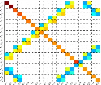
Figure 2: Illustration of stiffness matrixKlshowing the position of non-zero values, withNl=9 andNR=11

onαand have non-zero off-diagonal terms and unequal diagonal terms (even when α=0). A consequence of this is that the natural frequencies for thenθ-modes of a ring

with attached supports will split whenn=Nl/2. This is consistent with the so-called

splitting rules [6,7] which indicate that frequency splits occur when 2n/Nlis an integer. The vibrating gyroscope shown in Fig.1has eight supports (Nl =8) and operates in

145

the 2θ-mode (n=2), and so the number of supports does not split the 2θfrequencies. However, using eight supports will split the 4θ, 8θ, 12θ, . . . modes.

An example illustrating when non-zero coupling terms occur in the total stiffness matrix is shown in Fig.2 for the case when Nl = 9, NR = 11 and α , 0. Each

cell represents the calculated value in the total stiffness matrix — white cells indicate

150

zero values, shaded/coloured cells indicate non-zero values. The presence of coupling is clear. For example, the (n =)1θand (p =)8θ-modes, the (n =)4θ and (p =

)5θ-modes, and the (n=)2θand (p=)11θ-modes all couple because (n±p)/Nlare integers. Along the main diagonal, the stiffness values occur in equal pairs, except whenn=9 when the support legs induce frequency splitting. In practice the presence of coupling

155

Similar reasoning can be used to determine the overall mass matrix including

sup-160

port leg inertia. The total kinetic energy in the support legs is given by:

Tl= 1 2 ˙

hT

"

Ml Mbl

MblT NlmlI2×2

#

˙

h, (16)

where Ml is a 2NR ×2NR matrix having the same structure as Kl and whose first

diagonal terms have the same form as Eq. (15) but withkrandktreplaced byml. These terms are simply equal toNlml(n2+1)/(2n2) forn < Nl/2. All of the Ml terms can

be found by using the same replacement in the Appendix. The coupling effect of the

165

support masses on the kinetic energy is defined by:

Mbl=Nlml

" I2×2

02(NR−1)×2 #

. (17)

2.4. Electrostatic energy

As the mean radius of the electrodes is normally large compared to the nominal capacitor gap size, the electrode capacitors are approximated as parallel plate capaci-tors. The voltages applied across the inner and outer capacitors are denotedViandVo

170

respectively, and the electrostatic energy stored by a differential element of the parallel plate capacitor is given by:

dEc= 0V2

2d dAc, (18)

whereis the relative permittivity of the ring material,0is the absolute permittivity,V is the electrical potential across the electrode-ring capacitor,dis the gap size between the capacitor and the ring, and dAcis the differential capacitor area. The gap size

175

between the inner or outer capacitor and the ring depends of the nominal gap size (denoteddg) and the radial displacementw(θ), such that:

d=dg±w(θ). (19)

Substituting Eq. (19) in Eq. (18) and expanding the denominator of the resulting equation as a Taylor series in terms ofw/dggives:

dEc= 0V2

2dg NT X

k=0

(∓1)k w

dg

!k

dAc (20)

whereNT is the number of terms used in the Taylor series expansion.

180

The differential capacitor area dAcis defined as eitherlridθfor the inner capacitor orlrodθfor the outer capacitor, whereriandr0 are the inner and outer mean radii of the capacitor respectively.

Neighbouring electrodes are normally separated from each other by circumferential gaps to help isolate the electrodes and allow space for the support legs. These gaps are

185

capacitors is obtained by integrating (20) around the circumference of the ring. The total electrostatic energy is obtained by summing the energy from both electrodes and

190

results in:

Ec=A NT X

k=0

     

roVo2+(−1) k_r

iV_i2

dgk

Z 2π

0

wkdθ

      (21) with

A =0l

2dg

(22)

Using the Ritz expansion of the radial displacement (Eqs. (2) to (4)), Eq. (21) pro-vides a polynomial expansion for the electrostatic energy in terms of generalised coor-dinatesq(1)n ,q

(2)

n up to orderNT.

195

2.5. Equation of motion

Lagrange’s equation is used to determine the equation of motion of the supported ring resonator:

d dt

∂T

∂q˙j

!

+∂(Ur+Ul) ∂qj =

∂Ec ∂qj

. (23)

Using the results developed earlier, the equation of motion can be written as:

(Mr+Ml) ¨Λ+(Kr+Kl+Kc)Λ+F¯nl=Fb. (24)

In this expression, Fb =−(Mbr+Mbl) ¨zbrepresents the base excitation force ap-200

plied to the central ring hub, indicating that for a perfect unsupported ring, the ring centre displacement resulting from an applied shock only couples to the rigid body motion of the ring. The first two entries of this vector are equal to−(mr+Nlml) ¨zb

and all other entries are zero. F¯nl represents the nonlinear electrostatic force and is a polynomial function ofΛ. This term arises from differentiatingEcwith respect to

205

generalised coordinatesq(1)n ,q (2) n , i.e.:

¯

Fnl=

                              . . . . . . −APN_k=T₃ k(roV

2

o+(−1)kriV2i)

dgk

R2π

0 w

k−1_cosjθdθ

−APNk=T3

k(roV2o+(−1)kriVi2)

dgk

R2π

0 w

k−1_sinjθdθ . . . . . .                               . (25)

The linear electrostatic stiffness terms have been separated from the nonlinear elec-trostatic terms and are incorporated in the linear stiffness matrixKc. The linear terms

are evaluated by settingk=2 in (21) to yield diagonal matrix:

Kc=−2πA

roVo2+riV_i2

dg2

I. (26)

The linear electrostatic forces provided by the outer and inner capacitors change

210

matrix). This softening effect increases as the electrode voltages increase, and the overall stiffness matrix of the system can become negative, making the system unstable, if the voltage is sufficiently large.

Some observations regarding the nonlinear electrostatic force are:

215

• If the electrode voltages are chosen such thatroVo2=riVi2, all even power terms in the generalised coordinates (i.e.kodd) in Eq. (25) cancel out, thereby elimi-nating some coupling mechanisms.

• Different terms in the nonlinear electrostatic force expansion exhibit softening or hardening behaviour (e.g. hardening occurs whenriVi2>roVo2).

220

• The expression developed for the nonlinear electrostatic force can be expanded analytically, but becomes cumbersome as the number of terms in the Taylor se-ries expansionNT increases and the Ritz order of approximationNR increases. Symbolic calculation software can be used without much difficulty to generate high order terms and evaluate the required integral terms.

225

Equation of motion (24) is rewritten by pre-multiplying by matrix (Mr+Ml)−1and

including a modal damping matrixDto give:

IΛ¨ +DΛ˙ +ΩΛ+Fnl =

"

−z¨b

0

#

(27)

In this expression, matrixΩdefines the undamped linear natural frequencies (in-cluding linear electrostatic effects) of the modes provided the stiffness (Kl) and mass

(Ml) matrices associated with the supports are diagonal – this occurs if the number of 230

modes included in the model is relatively low (NR < Nl/2) or the linear coupling is simply neglected because it is small. For the device shown in Fig.1, which will be analyzed later, the stiffness and mass matrices contain coupling terms for the 4θ, 8θ, 12θ, . . . modes. However, this coupling can be avoided by selecting support leg angle α=0. Coupling also exists between different mode pairs, as discussed in the previous

235

section (see Fig.2). For example, coupling exists between 3θand 5θ-modes and this coupling can not be eliminated by selecting a particular value ofα. This coupling is neglected in the current study on the basis that it will be weak and to simplify the anal-ysis. The damping matrix Dis normally assumed to be diagonal and contains terms ωn/Qn, whereQn is the quality factor (or Q-factor) andωn is the undamped natural

240

frequency for each mode.Fnldefines the influence of the nonlinear electrostatic forces including any coupling between generalised coordinates.

In summary, the equation of motion for thenθ-mode can be expressed as:

¨

q(1)_n + ωn Qn ˙

q(1)_n +ω2_nq(1)_n +Fnlq(1)n =Fextq(1)n (28)

Similarly, the equation of motion for the companionnθorthogonal mode is obtained by replacingq(1)n byq

(2)

n in (28). The external forcesFext_q(1) 1

andFext_q(2) 1

correspond to

245

later studies by settingFext_q(1)

2 =cosωtto replicate standard operating conditions for a

Coriolis vibrating ring based gyroscope.

250

The nonlinear term Fnl_q(1)

n depends on the modal mass for then

th _{mode. For the} purpose of simplicity, the contribution from support leg inertia on this nonlinear term has been neglected in later numerical simulations. This simplification will have a small influence on the amplitude of the nonlinear force but the general behaviour illustrated in Section3will be unaffected.

255

In Eq. (28), the electrostatic force provides the only source of nonlinearity. Under standard operating conditions,Fnlcan be neglected on the basis that the displacement of the ring is small compared to the gap size. However, in this study severe shock conditions are investigated which induce ring displacement in the order of the nominal gap size, and it is necessary to model the nonlinear electrostatic forces. As described

260

earlier, the nonlinearity is expressed in power series form and the level of approxima-tion depends on the number of terms used in the Taylor expansionNT. The polynomial order of the nonlinear force isNT −1 and including these nonlinear forces introduces a physical mechanism for mode coupling to occur. Depending on the selected value of

NT, coupling can occur between several generalised coordinates.

265

3. Shock simulations

3.1. Simulation data

Numerical results are presented here for a recently reported device, manufactured and tested by Yoon et al. [1]. The dimensions of the ring are: mean radiusr=1.5mm,

radial thicknessh = 18µm, and axial lengthl = 150µm. The nominal gap between

270

capacitor and ring is dg = 10µm. The material properties are: Young’s modulus

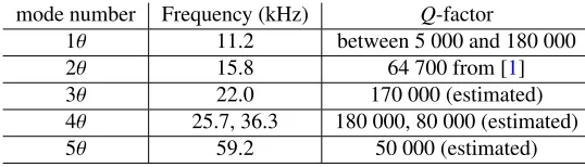
E = 150GPa and densityρ =2330kg/m3. The ring is supported by 8 pairs of legs. Using Eq. (28), the stiffnesses of the legs are accounted for within the natural frequen-ciesωn. These frequencies were obtained from a modal analysis of the resonator using a commercial Finite Element (FE) software package and the results are presented in

275

Table1. The electrostatic forces are quite week and in practice make only a small modification to the frequencies. On this basis it is justifiable to neglect their contribu-tion to the linear frequencies. The natural frequency calculated for the 2θ-mode (i.e. ω2) is in agreement with the results presented in [1]. The mode shapes obtained from the FE analysis forn ≤3 are shown in Fig.3. Moden=1 describes the 1θring rigid

280

body motion, whilst the other modes (n = 2, n = 3) describe the 2θand 3θflexural modes of the ring. The frequencies calculated for the 4θand 5θ-modes are provided. There are two 4θfrequencies because the eight support legs split the 4θfrequencies. In simulations, the high-frequency 4θ-mode is used as it aligns with the support legs and satisfies theα=0 condition. In practice, the modal analysis produces an assortment of

285

leg dominated modes in addition to the 1θ-mode, but these modes are not considered in the current model (28).

To simulate the dynamics of the gyroscope using Eq. (28), the damping for each mode is required and these are specified in (28) as Q-factors. TheQ-factors used in the simulations are presented in Table1and were obtained as explained below. The

290

(a) (b) (c)

Figure 3: Undeformed shape and deformed mode shape of the ring gyroscope for (a)n=1, (b)n=2 and (c)n=3.

mode number Frequency (kHz) Q-factor

1θ 11.2 between 5 000 and 180 000

2θ 15.8 64 700 from [1]

3θ 22.0 170 000 (estimated)

4θ 25.7, 36.3 180 000, 80 000 (estimated)

5θ 59.2 50 000 (estimated)

Table 1: Undamped natural frequencies and associatedQ-factors for the first five ring modes.

connecting the central hub to the device and thermoelastic damping. In numerical simulations, a range of values ofQ1 is used. The 2θ-mode Q-value was measured experimentally in [1] and the same value is kept within the simulations. TheQ-values for the other flexural modes were not presented in [1] and so were calculated based on

295

the assumption that thermoelastic damping is the only source of dissipation. The values presented in Table1were calculated using Zener’s theory [11]. Using this approach it can be shown [12] that theQ-factor of each ring mode can be calculated using:

1

Q=

1

Qr

Vr

Vr+Vl + 1

Ql

Vl

Vr+Vl

, (29)

whereQrandQlare respectively theQ-factors for the ring and legs considered inde-pendently (see Eq. (30)),VlandVrare respectively the energy stored in the support legs

300

and the ring for the mode considered – these quantities are obtain from an FE model of the undamped system.QrandQlare given by [12]:

Qr,l=

1+τr,lωi

2

∆M

(30)

whereωi is the fundamental undamped natural frequency of the supported ring for the mode considered, τr,l and ∆M are respectively the effective relaxation time and relaxation strength defined as:

305

τr,l=

Cvh2_r,l

kπ2 and ∆M=

Eα2T0

Cv

Herehr,lis either the radial ring thickness (hr =18µm) or the leg width (hl =10µm);

Cv =ρCp (withCp =700J.kg−1.K−1the specific heat for silicon) is the specific heat capacity at constant volume;k=130W.m−1_.K−1_{is the thermal conductivity for silicon;} α=2.6×10−6K−1is the coefficient of thermal expansion for silicon;T0=300K is the reference temperature.

310

The applied shock corresponds to an imposed acceleration of the base of the sensor and is accounted for in the definition of ¨zbin Eq. (27). In the model it is represented

as an applied external force on the 1θrigid body mode and will be referred to asFs later. The applied shock is assumed to be a half-sine pulse [13] and is applied along the α=0 direction to eliminate any coupling in the stiffness matrix. As such, acceleration

315

¨

zbis expressed as:

¨

zb= "

Fs 0

# =

          (

Assin_Tπt_s fort≤Ts 0 fort>Ts

0

         

, (32)

whereAsandTsare respectively the amplitude and duration time of the applied shock. Throughout the following study,Tsis chosen to be one tenth of the period of the 2θ-mode. In severe shock conditions, the amplitude of the shock can be very high and for the device analyzed the maximum amplitude considered is 10 000g (a shock of 15 000g

320

was applied by Yoon et al. in [1] but the shock duration was not mentioned) which causes the ring-electrode gap to reduce to approximately 60% of its nominal value. For higher levels of deformation the so-called ”pull-in” phenomenon [14] is likely to occur, in which the ring would be pulled into contact with the electrode. The developed model focuses on investigating the dynamic behaviour under nonlinear electrostatic forcing

325

and does not consider contact with the electrode.

The nonlinear coupling terms provide the only means of coupling the generalised coordinates. By aligning the external forcing withα=0, there is no coupling with the orthogonal companion modesq(2)n . This halves the number of generalised coordinates that need to be included in the equations of motion, and in what follows only

gen-330

eralised coordinatesq(1)n , corresponding to thenθ-mode, are considered without their orthogonal companion. To simplify notation, superscript (1) will be removed and the generalised coordinates considered will be referred to asqn.

Except when stated otherwise, the inner electrode is deactivated (Vi =0) in below simulations.

335

3.2. Preliminary study: influence of the nonlinear force order

As the applied shock considered is severe (As=10 000g), strong nonlinear effects are expected and the order of the Taylor series expansion (20) must be considered carefully to correctly predict these nonlinear effects. Initially a convergence study is performed to show the influence of using a different number of terms in the Taylor

340

series expansion for the nonlinear electrostatic force.

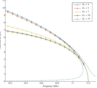
Figure 4 shows the backbone curve for the nonlinear 1θ-mode calculated using different values for the number of terms ofNT in the Taylor expansion. A nonlinear mode is defined as a harmonic solution of the underlying autonomous conservative system of Eq. (27):

345

The Harmonic Balance Method (HBM) is employed to calculate the nonlinear mode (see [15] for a detailed explanation how to compute nonlinear modes). Non trivial solution of Eq. (33) are sought in the form of a Fourier ansatz:

Λ(t)=a0+

Nh X

k=1

akcos(kωt)+bksin(kωt), (34)

whereNhis the number of harmonics retained. Inserting Eq. (34) into (33) and eval-uating Fourier-Galerkin projections with respect to the base functions gives rise to a

350

system of nonlinear algebraic equations with unknownsa0,ak,bkandω(k∈J1,NhK). To determine the nonlinear 1θ-mode, this system of equations is solved by an arc-length continuation scheme [16] initiated with the linear frequencyω1and a small value ofΛ.

10.2 10.4 10.6 10.8 11 11.2

0 1 2 3 4 5 6 7 8 9 10 11

Frequency (kHz)

Amplitude

q1

(

µ

m)

NT=4

NT=5

NT=7

NT=10

NT=15

Figure 4: Nonlinear normal modeq1for different values ofNT

At low energy levels (low amplitude), the natural frequency of the nonlinear mode is equal to the linear natural frequency (11.2kHz for the 1θ-mode). However as the

355

The advantage of studying nonlinear modes is that they show how the loci of the maximum response changes under harmonic forcing. This is depicted in Fig.4 by

360

frequency response functions (FRFs) plotted on top of the nonlinear modes. FRFs of the system forNT = 4 – dashed lines, and NT = 10 – dotted lines, are illustrated. These forced responses were obtained using arbitrary (but equal) forcing amplitudes to demonstrate that the bent peak follows the nonlinear modes. It is clear that de-pending on theNT-value, the response, be it forced or free, is different. Convergence

365

for a maximum amplitude of approximately 6µm (corresponding to the 60% gap size displacement under applied severe shock) is obtained forNT ≥10.

In the following simulations, the number of terms in the Taylor series will be se-lected to beNT =10, corresponding to a polynomial nonlinear force of order 9.

3.3. Free response after shock: influence of the number of modes

370

In the first set of simulations, the resonator is considered to be at rest initially and is then subjected to a 10 000gshock onq1att=0 as defined in Eq. (32). The amplitude of the shock is large and causes the ring-electrode gap to reduce to approximately 60% of its nominal value.

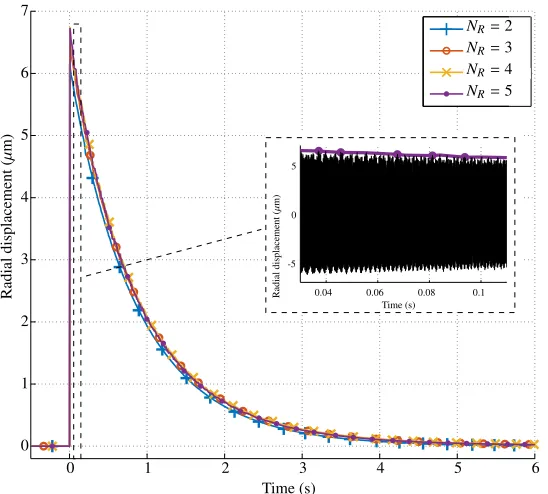
Figure 5 illustrates the radial displacement (defined in Eq. (2)) as a function of

375

time for different Ritz orders of approximationNR. For clarity, only the positive en-velope of the response time-history is plotted to illustrate the global behaviour of the response over several seconds. The envelope was calculated by identifying local max-ima in short duration windows of the multi-frequency time-history and then manually combining and refining these maxima to achieve maxima points that encapsulate the

380

global response behaviour. A sample showing the time response and positive envelope is illustrated as an embedded figure in Fig.5for a zoom on theNR=5 simulation. The results in Fig.5 show that the radial displacement envelope after shock is accurately simulated using the first 3-modes of vibration (rigid body motion and 2θand 3θ flex-ural modes). The main reason for this is that the modal amplitude decreases quickly

385

as the mode number increases and theq1response dominates the response amplitude. ForNR = 5, direct linear coupling between theq5 andq3 coordinates caused by the extra-diagonal terms inKlandMlmatrices has been neglected.

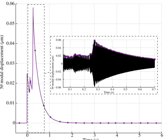
Fig.6shows the positive envelope for modal amplitudeq5calculated withNR =5 together with a sample showing the time response and positive envelope for a zoom

390

on the simulation. The results show a non-smooth behaviour and a rapid increase in amplitude att ≈ 0.28s. To fully understand this singularity in the response, it is instructive to consider the evolution of the frequencies contained in the response over time. This is achieved by computing the spectrogram of the modal displacements. To calculate the spectrograms, the time-varying response is segmented into short periods

395

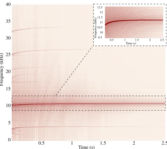
and an FFT-based spectral estimate is performed over sliding windows [17]. The color and shades of the spectrograms encode frequency power levels. Dark color indicates frequency content with higher power, and a strong line (or ray) indicates for instance the existence of a particular frequency and shows its evolution over time. Figs.7and8 show spectrograms for theq1andq5responses, respectively.

400

0 1 2 3 4 5 6 0

1 2 3 4 5 6 7

Time (s)

Radial

displacement

(

µ

m)

NR=2

NR=3

NR=4

NR=5

0.04 0.06 0.08 0.1

-5 0 5

Time (s)

Radial

displacement

(

µ

m)

Figure 5: Shock simulations with structure initially at rest. Positive envelope of the radial displacement for different values ofNR.

known to be a consequence of nonlinear effects. The zoom shows howω1 slowly in-creases over time from 10.6kHz to 11.2kHz as amplitudeq1decays. This behavour is

405

caused by the softening effect of the nonlinear forces which also explains the increase in frequency over time of combinations of harmonics.

Figure 8shows even richer dynamics. In addition to the different harmonics or combination of harmonics, there is clear evidence of modal interaction att≈0.3s and ω≈60kHz. This modal interaction occurs whenω5 =2ω1+ω2+ω3 and creates an

410

additional means of mode coupling. This energy exchange induces a peak in theq5 response (see Fig.6), but as the amplitude is relatively small compared to the ampli-tude ofq1, the peak is not visible in the global response of Fig.5. Depending on the resonator dimensions, additional modal interactions are expected to occur.

3.4. Forced harmonic response with applied shock

415

Under operating conditions, one of the 2θ-modes of a vibrating gyroscope is driven at resonance and the response of the companion 2θ-mode is measured to provide a measure of the angular rate [18]. In this section the conditions when an applied shock significantly affects the forced vibration of the 2θ-mode via inter-modal coupling are investigated when there is no applied rate.

420

A constant amplitude harmonic force is applied to the 2θ-mode i.e.Fextq2 =Aecosωt

0 1 2 3 4 5 6 0

0.01 0.02 0.03 0.04 0.05 0.06

Time (s)

5

θ

modal

displacement

(

µ

m)

0.1 0.2 0.3 0.4 0.5 0.6 0.7

0 0.02 0.04 0.06

Time (s)

5

θ

modal

displacement

(

µ

m)

- 0.06 - 0.04 - 0.02

Figure 6: Shock simulations with structure initially at rest. Positive envelope of the modal displacementq5

calculated withNR=5.

chosen such that the drive amplitudeq2 is approximately 4% of the nominal gap size (≈0.4µm) and three modes (NR=3) are sufficient to characterize the global dynamics,

425

see Section3.3. In a way similar to the calculation of the nonlinear mode (see Sec-tion3.2), the nonlinear response curve was found using a Harmonic Balance Method (HBM) that solves directly for the harmonic steady-state solutions, combined with an alternating frequency-time procedure (AFT) [19] to compute the projection of the non-linear forces in the frequency domain, and arc-length continuation techniques [16] to

430

follow a continuous branch of solution as the excitation frequency varies. Due to the presence of nonlinearity, the system presents two stable solutions over some frequency ranges, the top and bottom branches on Fig.9. The results illustrate the softening behaviour of the nonlinear forces.

In the following simulation case studies, the 2θ-mode only is driven at a frequency

435

close to the peak of the nonlinear resonance (the actual frequency corresponds to the marker shown in Fig.9,w ≈ 15.7983kHz). Initially the system is maintained at its top stable branch solution (q2 ≈0.39µm). A shock is then applied to the 1θ-mode, at

t = 0s. The shock causes the ring to vibrate as a rigid body but also influences the flexural vibration of the 2θ-mode because of the coupling provided by the nonlinear

440

40

35

30

25

20

15

10

5

0

0.5 1 1.5 2 2.5

Time (s)

Frequenc

y

(kHz)

Frequenc

y

(kHz)

9.5 10 10.5 11 11.5 12 12.5

Time (s)

0.5 1 1.5 2 2.5

Figure 7: Shock simulations with structure initially at rest. Spectrogram of theq1response calculated with

NR=5.

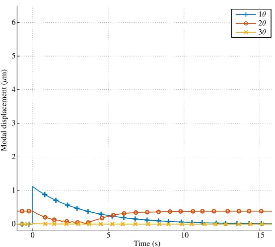
Case 1. For this case the shock amplitude is relatively small (As=2 000g) and 1θ

445

damping low (Q1 =120 000), and the results are shown in Fig.10. After a short tran-sient response of approximately 7s, the system returns to its initial conditions whereq2 is at its top stable branch (round marker in Fig.9).q1shows a slow exponential decay from damping.

450

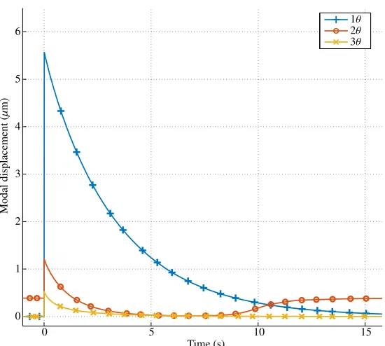
Case 2. In this case the shock amplitude is large (As=10 000g) and the damping

low (Q1 =120 000). Due to the increased shock amplitude, which increases the ring deformation to 55% of its nominal gap size, the choice of NT-value is important to achieve convergence, see Section3.2. The results are shown in Fig.11, where it can be seen thatq2 displays particularly interesting dynamic behaviour. After an initial

455

transient response (up to approximately 5s),q2appears to stabilise on its bottom branch

q2 ≈0.03µm (yellow cross marker of Fig.9). However, whileq1displacement slowly decays due to damping,q2returns to its initial condition on the top stable branch.

Case 3. In this case the shock amplitude is large (As = 10 000g as in Case 2)

but the damping on the 1θ-mode is increased by a factor of 3 (Q1 = 40 000). The

460

0.5 1 1.5 2 2.5 Time (s)

70

60

50

40

30

20

10

0

Frequenc

y

(kHz)

Figure 8: Shock simulations with structure initially at rest. Spectrogram of theq5response calculated with

NR=5.

15.7960 15.797 15.798 15.799 15.8 15.801 15.802 0.05

0.1 0.15 0.2 0.25 0.3 0.35 0.4

Frequency (kHz)

Modal

displacement

q2

(

µ

m)

0 5 10 15 0

1 2 3 4 5 6

Time (s)

Modal

displacement

(

µ

m)

1θ 2θ 3θ

Figure 10: Positive envelope of the modal displacements as a function of time after a small shock – Case 1.

q2 stabilises and remains on the bottom stable branch. These results demonstrate the jump phenomenon from one branch to the other, as depicted by the arrow in Fig.9.

Case 4. In this case the conditions necessary to cause the jump phenomenon

ob-465

served in Case 3 are investigated by varyingQ1. As in Case 3, the shock amplitude is large butQ1is varied from 5 000 to 180 000. The results for the 2θresponse only are shown in Fig.13. These results confirm the previous findings where theq2 solu-tion jumps to the bottom branch when the damping is high (lowQ1-value) but returns to the top branch after a sufficient stabilisation time when the damping is low (high

470

Q1-value).

The main conclusion drawn from this case studies is that for particular values of shock amplitude and damping the system exhibits jump behaviour from the high ampli-tude resonant driving state to a much lower ampliampli-tude. Even if the 2θdrive amplitude is maintained initially, a shock applied to the rigid body 1θ-mode can cause the ring

475

amplitude to reduce suddenly. The jump phenomenon is caused by coupling between modes of vibration created by nonlinear effects that are normally not accounted for at the design stage. Furthermore, it has been shown that the abrupt jump down only occurs for high 1θdamping levels, which are often considered to be desirable as they quickly damp the rigid body motion. In practical applications, a control system may be

480

0 5 10 15 0

1 2 3 4 5 6

Time (s)

Modal

displacement

(

µ

m)

1θ 2θ 3θ

Figure 11: Positive envelope of the modal displacements as a function of time for a severe shock – Case 2.

the required steady-state amplitude.

3.5. Influence of the inner electrode

In all previous simulations, the inner voltage was set equal to 0 to simulate ring

485

resonators with outer electrodes only. To gain some understanding of the benefits or otherwise of using inner as well as outer electrodes, it is necessary to reconsider the equations of motion. With the assumption thatNR =2, andNT =5, the equations of motion (28) can be expressed as:

      

¨

q1+ω_Q1

1q˙1+ω1

2_q

1+αq1q2−βq1(q12+2q22)+γq1q2(4q2₁+3q2₂)=Fs ¨

q2+ω_Q2

2q˙2+ω2

2_q

2+4₅αq2₁−₅8βq2(q22+2q12)+4₅γq2₁(2q2₁+9q2₂)=0

, (35)

with:

α= 3(riV

2 i −roV

2 o)Aπ (mr+8ml)dg3

, β= 3(riV

2 i +roV

2 o)Aπ (mr+8ml)dg4

, γ= 5α

6d2 g In this expression, there is no harmonic forcing applied to the 2θ-mode.

490

As mentioned in Section2.5, imposing the conditionriV_i2 =roVo2causes all of the even order terms in the nonlinear force expression to cancel out and eliminates some coupling mechanisms. Under these conditions the nonlinear force terms only include odd order terms and the above equation simplifies to:

( _q¨

1+ω_Q1₁q˙1+ω12q1−βq1(q12+2q22)=Fs ¨

q2+ω_Q2₂q˙2+ω22q2−8₅βq2(q22+2q12)=0

0 5 10 15 0

1 2 3 4 5 6

Time (s)

Modal

displacement

(

µ

m)

1θ 2θ 3θ

Figure 12: Positive envelope of the modal displacements as a function of time for a severe shock but with high damping – Case 3.

These equations indicate that if the system has zero initial conditions when the shock

495

is applied, there is no coupling betweenq1andq2andq2=0 is the solution to Eq. (36) for all values oftand allFs. This means that a shock applied toq1will not exciteq2. Simulation results for this case are shown in Fig.14and were obtained usingNR =3 andNT = 10. These results confirm that the applied shock does not produce anyq2 response for a more general form of equations. This phenomenon of ”no coupling

500

when the inner and outer voltages are symmetric” was previously mentioned in [4]. For the case when the initial conditions forq2are non-zero, like those considered in Section3.4where the 2θ-mode is harmonically excited, the shock produces some cou-pling between generalised coordinates. Simulation results illustrating this behaviour are shown in Fig.15. The results show the positive envelopes of the modal

displace-505

ments after the applied shock with a harmonic forcing applied toq2. It can be seen thatq2 varies after the shock is applied and shows a jump behaviour similar to those illustrated in Fig.13. A nonlinear modal interaction betweenq1 andq3 is also seen at approximatelyt = 0.1s when there is a sudden increase inq3 and decrease inq1, indicating the transfer of vibrational energy from nonlinear coupling betweenq1 and

510

0 5 10 15 0

0.2 0.4 0.6 0.8 1 1.2

Time (s)

2

θ

modal

displacement

(

µ

m)

Q1=5000

Q1=40000

Q1=80000

Q1=120000

Q1=180000

Figure 13: Positive envelope of theq2modal displacement as a function of time for a severe shock and

different values of damping – Case 4.

4. Conclusions

A mathematical model has been developed and used to investigate the dynamic behaviour of ring resonators under severe shock conditions and nonlinear electrostatic forcing. The model describes the ring response in terms of the modes of a perfect ring,

515

indicates that the nonlinear electrostatic forces induce mode coupling, and is used to simulate the resulting physical response.

The nonlinear electrostatic force was approximated using a Taylor series expan-sion and a study was performed to investigate the order of approximation required to achieve converged results. For the severe shocks considered, when the electrode gap

520

reduces by∼ 60%, it is necessary to use a 9th order approximation of the nonlinear electrostatic force and three modes of flexural vibration (1θ, 2θand 3θ) to achieve con-verged results for the global shock behaviour. Only three modes are required because the ring natural frequencies are well separated from each other; higher order modal responses decay quickly; and there is no linear coupling between the first ring modes.

525

Electrostatic nonlinearity introduces coupling between the modes such that a shock which principally excites the rigid body mode produces flexural vibration of the ring and induces coupling between the 1θand other modes. Under severe shock conditions sensor performance deteriorates compared to the linear case (without coupling). Fur-thermore, under operating conditions when the 2θmode is driven at resonance, it was

530

0 10 20 30 40 50 60 0

1 2 3 4 5 6

Time (ms)

Modal

displacement

(

µ

m)

1θ 2θ 3θ

Figure 14: Positive envelopes of the modal displacements as a function of time for a severe shock without other external forces and with a symmetrical electrodes effect.

of this phenomenon is mainly a function of shock amplitude and rigid-body motion damping and is likely to reduce sensor performance momentarily. Finally, by incor-porating both inner and outer electrodes the electrostatic restoring force can be made

535

symmetric. This removes some coupling mechanisms between modes, but does not remove all couplings if the shock occurs when the resonator is vibrating.

A detailed analysis (bifurcation condition and stability studies) could be performed to more fully understand the complex dynamics created by the nonlinear electrostatic force. Experimental measurements on CVG devices under severe shock conditions are

540

also required to validate the findings and further investigate the conditions when the jump phenomenon occurs. It is anticipated that the model and results presented will guide future development of high performance capacitive CVGs.

Acknowledgement

The authors acknowledge the International Exchanges Scheme - Cost Share

Pro-545

0 5 10 15 0

1 2 3 4 5 6

Time (s)

Modal

displacement

(

µ

m)

1θ 2θ 3θ

Figure 15: Positive envelope of the modal displacements as a function of time for a severe shock under harmonic forcing and with symmetrical electrodes effect.

References

[1] S. Yoon, U. Park, R. J., S. Yang, Tactical grade mems vibrating ring gyroscope with high shock reliability, Microelectronic Engineering 142 (2015) 22–29.doi:

550

10.1016/j.mee.2015.07.004.

[2] A. D. Challoner, H. H. Ge, H. Y. Liu, Boeing disc resonator gyroscope, Posi-tion, Location and Navigation Symposium - PLANS 2014, IEEE/ION, Monterey, USA, 2014.doi:10.1109/PLANS.2014.6851410.

[3] S. Yoon, S. Lee, K. Najafi, Vibration sensitivity analysis of mems vibratory ring

555

gyroscopes, Sensors and Actuators, A: Physical 171 (2011) 163–177. doi:10.

1016/j.sna.2011.08.010.

[4] S. Sieberer, A. A. Popov, S. McWilliam, Shock-induced electrostatic coupling of modes of vibration in the response of a mems ring sensor, IDETC/CIE, Chicago, USA, 2012.doi:10.1115/DETC2012-70915.

560

[5] S. Sieberer, In-plane shock response of capacitive mems ring-rate senors, Ph.D. thesis, The University of Nottingham (2014).

[6] C. Fox, A simple theory for the analysis and correction of frequency splitting in slightly imperfect rings, Journal of Sound and Vibration 142 (3) (1990) 227–243.

doi:10.1016/0022-460X(90)90554-D.

[7] S. McWilliam, J. Ong, C. Fox, On the statistics of natural frequency splitting for rings with random mass imperfections, Journal of Sound and Vibration 279 (1-2) (2003) 453–470.doi:10.1016/j.jsv.2003.11.034.

[8] F. Ayazi, K. Najafi, A HARPASS polysilicon vibrating gyroscope, Journal of Mi-croelectromechanical Systems 10 (2001) 169–179. doi:10.1109/84.925732.

570

[9] Z. X. Hu, B. J. Gallacher, J. S. Burdess, C. P. Fell, K. Townsend, Precision mode matching of MEMS gyroscope by feedback control, Limerick, Ireland, 2011.

doi:10.1109/ICSENS.2011.6126998.

[10] A. E. Love, A treatise on the mathematical theory of elasticity, 4th_Edition, Cam-bridge University Press, 2013.

575

[11] C. Zener, Internal friction in solids I. theory of internal friction in reeds, Physical Review 52 (3) (1937) 230–235. doi:10.1103/PhysRev.52.230.

[12] S. T. Hossain, Thermoelastic damping and support loss in MEMS ring resonators, Ph.D. thesis, The University of Nottingham, UK (2016).

[13] V. T. Srikar, S. D. Senturia, The reliability of microelectromechanical

sys-580

tems (mems) in shock environments, Journal of Microelectromechanical Systems 11 (3) (2002) 206–214. doi:10.1109/JMEMS.2002.1007399.

[14] W.-M. Zhang, H. Yan, Z.-K. Peng, G. Meng, Electrostatic pull-in instability in mems/nems: A review, Sensors and Actuators, A: Physical 214 (2014) 187–218.

doi:10.1016/j.sna.2014.04.025.

585

[15] M. Peeters, R. Vigui´e, G. S´erandour, G. Kerschen, J. C. Golinval, Nonlinear nor-mal modes, part ii: Toward a practical computation using numerical continuation techniques, Mechanical Systems and Signal Processing 23 (1) (2009) 195–216.

doi:10.1016/j.ymssp.2008.04.003.

[16] E. Sarrouy, J.-J. Sinou, Non-Linear Periodic and Quasi-Periodic Vibrations in

590

Mechanical Systems - On the use of the Harmonic Balance Methods, Advances in Vibration Analysis Research, InTech, 2011, pp. 419–434.doi:10.5772/15638.

[17] MATLAB, version 8.3.0 (R2014a), The MathWorks Inc., Natick, Massachusetts, USA, 2014.

[18] C. H. J. Fox, D. J. W. Hardie, Vibratory gyroscopic sensors, DGON Symposium

595

Gyro Technology, Stuttgart, 1984, pp. 13.0–13.30.

Appendix

600

K_ljis composed ofK_lj_n,pmatrices (size [2×2]) at rows (2n−1,2n) and columns (2p−1,2p), with 1<n<NRand 1<p<NR.

K_lj=                      . . . . . . . .

K_lj_n,p

. . . . . . . .                      (37)

One introduces here an angleαthat defines the position of the last leg with respect to the global frame. This angle can be arbitrarily taken. SubstitutingΨ2_Njπ

l +α

by its value (3) in (13) gives :

605

K_lj_n,p=       

kraccj + kt

npa j

ss kracsj − kt

npa j sc

kra j sc−_npkta

j cs kra

j ss+_npkta

j cc        (38) with :

accj =cos 2n jπ

Nl +

nα

!

cos 2p jπ

Nl +

pα

!

(39)

assj =sin 2n jπ

Nl +

nα

!

sin 2p jπ

Nl +

pα

!

(40)

acsj =cos 2n jπ

Nl

+nα

!

sin 2p jπ

Nl

+pα

!

(41)

ascj =sin 2n jπ

Nl

+nα

!

cos 2p jπ

Nl

+pα

!

(42)

In order to calculate the total strain energy (12), one needs to calculatePNl

j=1a cc

j,

PNl

j=1a ss j ,

PNl

j=1a cs

j and

PNl

j=1a sc

j . This derivation follows.

Nl X

j=1

acc_j =

Nl X

j=1

cos 2n jπ

Nl

+nα

!

cos 2p jπ

Nl

+pα

!

= 1

2 Nl X

j=1

"

cos 2(n+p)jπ

Nl

+(n+p)α

!

+cos 2(n−p)jπ

Nl

+(n−p)α

!#

(43)

Utilising the fact that:

Nl X

j=1

cos 2n jπ

Nl

+nα

! =

(

Nlcosnα ifn/Nl∈Z

Equation (43) gives :

Nl X

j=1

acc_j =

              

Nl

2 cos(n−p)α if (n−p)/Nl∈Zand (n+p)/Nl<Z Nl

2 cos(n+p)α if (n−p)/Nl<Zand (n+p)/Nl∈Z

Nlcosnαcospα if (n−p)/Nl∈Zand (n+p)/Nl∈Z

0 otherwise.

(45)

A similar reasoning can be performed for PNl

j₌1a ss j,

PNl

j₌1a cs j , and

PNl

j₌1a sc j . The

610

value of each sum depends of some conditions on the row and column number (nand

prespectively). These are summaries below.

P _{Condition onpandn}

(n−p)/Nl∈Z (n−p)/Nl<Z (n−p)/Nl∈Z otherwise and (n+p)/Nl<Z and (n+p)/Nl∈Z and (n+p)/Nl∈Z

position inKl positive diag. negative diag. intersection of diag. everywhere else

PNl

j=1a cc j

Nl

2cos(n−p)α Nl

2 cos(n+p)α Ncosnαcospα 0

PNl

j=1assj Nl

2cos(n−p)α − Nl

2cos(n+p)α Nsinnαsinpα 0

PNl

j=1acsj −Nl2sin(n−p)α Nl2 sin(n+p)α Ncosnαsinpα 0

PNl