TRANSLATION OF APL TO OTHER HIGH-LEVEL
LANGUAGES
Margaret M. Jacobs
A Thesis Submitted for the Degree of PhD
at the
University of St Andrews
1975
Full metadata for this item is available in
St Andrews Research Repository
at:
http://research-repository.st-andrews.ac.uk/
Please use this identifier to cite or link to this item:
http://hdl.handle.net/10023/13417
The code generated corresponding to a particular APL routine will not
at first be very efficient. However, methods of optimising the generated
code are discussed at length in the thesis. A brief comparison is made
with other possible methods of conversion.
There are certain restrictions on the types of APL statements able to be
handled by the translation method. These restrictions a/re listed in an
accompanying appendix.
Throughout the text, several examples are given of the code which will
be generated from particular APL statements or expressions. Some more
lengthy examples of conversion of APL routines to FORTRAN are provided as
HIGH-LEVEL LANGUAGES
The research work required to produce this thesis was carried out in
the Department of Computational Science, University of St. Andrews.
Financial assistance was provided by the Science Research Council.
The thesis describes a method of translating the computer language
APL to other high-level languages. Particular reference is made to
FORTRAN, a language widely available to computer users. Although gaining
in popularity, APL is not at present so readily available, and the main aim
of the translation process is to enable the more desirable features of APL
to be at the disposal of a far greater number of users. The translation
process should also speed up the running of routines, since compilation in
general leads to greater efficiency than interpretive techniques. Some
inefficiencies of the APL language have been removed by the translation
process. The above reasons for translating APL to other high-level
languages are discussed in the introduction to the thesis.
A description of the method of translation forms the main part of the
thesis. The APL input code is first lexically scanned, a process whereby
the subsequent phases are greatly simplified. An intermediate code form
is produced in which bracketing is used to group operators and operands
together, and to assign priorities to operators such that sub-expressions
will be handled in the correct order. By scanning the intermediate code
form, information is stacked until required later. The information is
used to make possible a process of macro expansion. Each of the above
processes is discussed in the main text of the thesis. The format of all
information which can or must be supplied at translation time is clearly
>
To
high-level languages, with particular reference to FORTRAN.
The work for this project was carried out in the Department of
Computational Science, University of St. Andrews, for the degree
The research for the subject matter of this thesis has been
carried out by myself, and the thesis has been composed by
myself. The thesis has not been accepted in fulfilment of
the requirements of any other degree or professional
I would like to thank Professor A.J. Cole for his excellent
supervision of my work throughout the course of my studies in St.
Andrews and for his advice on the preparation of my thesis.
I am extremely grateful to all the members of staff of the John
Honey Building at the University of St. Andrews for their willing
assistance and encouragement, and to my fellow research students for
their helpful comments.
I also must thank Mrs. V. Butterworth for typing the text of my
C O N T E N T S
page
INTRODUCTION 1
Chapter
I INPUT PHASE AND METHOD OF STORAGE ALLOCATION ' 5
II LEXICAL SCANNING- PHASE 31
III RIGHT-TO-LEFT SCAN AND PRODUCTION OF INTERMEDIATE CODE 59
IV LEFT-TO-RIGHT SCAN, PRODUCTION OF STACKED INFORMATION 76 AND ORGANISATION OF MACRO EXPANSIONS
V THE MACRO METHOD 109
VI LABELS AND JUMPS 154
VII PROCESSING OF INITIAL INFORMATION I 61
VIII CODE OPTIMISATION 1?1
Appendix
1 SYMBOLS USED FOR INPUT OF APL DURING TESTING
2 TABLE OF USEFUL INFORMATION FOR APL OPERATORS
3 LIST OF MACRO INSTRUCTIONS AND THEIR FUNCTIONS
4 LIST OF MACRO BODIES
5 COMPARISON OF BRACKETING METHOD AND REVERSE POLISH METHOD
6 RESTRICTIONS
7 EASE OF CONVERSION TO OTHER LANGUAGES
8 FUNCTION OF GLOBAL VARIABLES (RUN-TIME)
9 EXAMPLES OF CONVERTED ROUTINES
The following text describes a method of translation of APL to other
high-level languages. The version of APL able to be translated is that
described in the IBM APL 360-OS and APL 360-DOS User's Manual, with a few
restrictions. These restrictions are listed in Appendix 6.
Throughout the text, the target language is assumed to be FORTRAN, but
similar techniques can be applied to translate from APL to ALGOL or to Pl/1.
In generating the target language code, only a subset of the permissible
FORTRAN statements has been used. The subset was chosen such that its
members (as far as possible) have counterparts in ALGOL and Pl/1. This
facilitates conversion to either of these languages instead of FORTRAN.
The ease of conversion to ALGOL or to Pl/1 is discussed in Appendix 7•
The translation was intended in the first place to handle conversion
of APL subroutines and functions, but main programs may also be translated.
The APL routines are not intended to remain interactive after conversion,
but to be run under a batch-processing system.
There have previously been some attempts to produce a batch-processor
for APL. One such attempt was made by H. Van Hedel, who implemented an
APL batch-process or in Pl/1 for the IBbl/36st). The only restriction he imposed was that function names and local variable names should be distinct.
(This restriction, among others, has been placed on the types of APL
state-7
ments able to be converted to FORTRAN.) In Van Hedel the following example
2
Vr <-f i
x
R < ~ @ X V
V & 1 ; F1
H
V
V G2
h V
Y h
Z <- F1 -A
V
Such an example creates ambiguity in the source text, for H returns differ
ent values in G-1 and G-2 .
For an interactive interpreter it is important that each operation is
executed as soon as sufficient information is gathered. For a
batch-processor, as much as possible of the analysis has to be done before the
execution takes place.
The above example is ambiguous to a compiler, but not to an interpreter.
It is intended that only working routines be converted to other languages.
Thus, the amount of checking required during conversion is greatly reduced. It
can be assumed, for example, that all dimensions are conformable in matrix
operations.
The reasons behind the translation (see Sayers^) are as follows;
(i) It is intended to provide a more easily transportable system. There
are at present more FORTRAN compilers than APL interpreters. Since
APL is highly suited to the development of algorithms (Smillie^), it would
be very convenient to be able to use these algorithms on a larger scale.
same argument can be applied to the translation of APL to ALG-OL or PL/1. )
To make transport of the converted routines as convenient as possible,
the user is provided with an option to specify the output medium for the
converted routines.
(ii) A secondary aim was to improve run-time efficiency by using compilation
rather than interpretation. The amount of code to be interpreted is
reduced if the user supplies some information about non-scalar variables.
The more information supplied, the greater the amount of compilation possible.
In many cases, the types and dimensions of variables will not change, and
such examples readily lend themselves to the improvement of run-time effic
iency. The method of supplying extra information to improve run-time
efficiency is described in Chapter I.
(iii) It is hoped that code can be optimised during the course of translation
by the removal of some of the inefficiencies of APL. An example of
an inefficient APL expression is
4 4* A+B
where A and B are non-scalar. This is obviously inefficient as all the
elements of A and B are summed, whereas only four summations are essential.
The method of removing the above inefficiency is outlined in the following text.
In December, 1971, V.L.Moruzzi gave a set of simple rules for translating
from APL to FORTRAN by hand. He estimated that mechanical APB/FORTRAN trans- ■
lations could achieve a 3,^-fold reduction in CPU time. This is discussed in
.3 Moruzzx .
At a private meeting, Dr. J.L.Alty of Liverpool University remarked that,
after visiting various APL installations in the U.S.A. and Canada, he found
APL three to four times faster than-other languages for program development,
emphasized the need for interchangeability between APL and other languages.
The translation from APL to FORTRAN is effected by a series of macro
expansions. The order of expansion of macros is determined by the order
of the operators in the APL source test.
A system of bracketing was introduced to ensure that all operators
(and hence macro expansions) would be assigned the correct priorities. ■
Reverse polish techniques could also have been applied during the trans
lation process. The rival merits of each method are discussed in Appendix 5»
The options available to the user are discussed in Chapter I, together
with the method of storage allocation. A lexical scan of the APL source
text is first carried out to simplify the subsequent processes. The lexical
scanning phase is discussed in Chapter II. Brackets are then introduced
during a right-to-left scan ox* the code and an intermediate code form is 3et
up. This is discussed in Chapter III. Stacking of information to be used
as parameters fox'* macros is described in Chapter IV, while the macro method
itself is dealt with in Chapter V. A discussion of labels and jumps is
given in Chapter VI, while Chapter VII describes the pre-optimisation phase.
A process whereby the generated code can be optimised has been devised. It
is described in Chapter VIII.
The APL-FORTRAN translator is written entirely in FORTRAN.
Definitions of the names used in the following text are given in
CHAPTER I
INPUT PHASE AND METHOD OP STORAGE ALLOCATION
APL routines to be converted to PORTRAN are read, line by line, into
a character array LINE. The routines are preceded by some additional
information. Some of the information provided is essential to the
conversion method (see §1.3) 3 and some can be provided as a user option (see §1.4) .
Most of the additional information supplied relates to the use of
non-scalar variables. The conversion routines use a fairly complicated
method of storage allocation for non-scalar variables. The method is
necessarily complicated as the dynamic storage capability of an APL
interpreter has to be simulated. The storage allocation method is
discussed in detail in §1.2 . The subsequent accessing of non-scalar
variables is necessarily time-consuming, as interpretive techniques have
to be employed. However, under certain circumstances, a simpler storage
allocation method can be employed, which reduces the access time for non
scalars considerably. The simpler method is only possible if the user
supplies additional information about his non-scalar variables.
A set of APL routines can be converted to PORTRAN during one run of
the conversion program. A calling program can be supplied with a set of
subroutines cr functions, but this has limited use in practice as the user
of the converted routines may want results for several different parameter
sets. Only one set of information is supplied initially for non-scalars,
6
V
A FN B ; XV
V
y Y ; XV
If FN and F are to be translated during a single run of the
conversion routines, then the types of X in both subroutines must be
the same. That is, if X is declared to be non-scalar at the start,
it will be assumed non-scalar in each subroutine. There is no serious
restriction when X is required to be scalar in one subroutine and non-
scalaz* in another. The problem is easily solved by changing the variable
name X in one or the other of the two routines. No problem would arise
if X was a global variable, as its type would be the same in both FN
and F .
Additional information must be supplied for both literal and numeric
non-scalars. All information supplied is printed out. It should be noted
that declarations should be supplied only for those variables which are non
scalar at their first occurrence. Otherwise, scalar occurrences of the
variables would not be recognised as such.
1.1 Input of the APL Source Program
The source program is assumed initially to be in APL internal Z-code
form. The program is read in and converted line by line. Each line is
stored in turn in the character array LINE, which is accessed during the
use an input form more suited to the character set of the IBM 029 card
punches. As far as possible, APL symbols were represented by their
counterparts on the keyboard of the IBM 029 card punch. Composite
symbols were used to represent the extraneous APL symbols. The actual
representation of the APL character set used during testing is shown in
Appendix 1. The symbols were then converted as required to APL internal
2-code form.
Under normal running conditions, the input would, of course, be in
APL internal Z-code form.
1*2 Method of Storage Allocation
The amount of storage space allocated for an APL non-scalar variable
can vary dynamically. The facility of dynamic storage allocation is not
available in FORTRAN. For this reason, it was necessary to simulate the
feature in the FORTRAN code produced. An arbitrary amount of storage
space (represented by array YSTOKS) vfas thus set aside for storage of all
non-scalar variables, and storage space is allocated as required for
individual non-scalar variables.
Since storage is allocated dynamically, a method had to be devised
of linking together the various blocks of YSTORE associated with a particular
non-scalar. It was obviously not advisable to link together individual
locations, as the cost in terms of storage space and access time would have
been prohibitive. Thus the array YSTORS was treated as separate units
of 10 locations each. The number was chosen as an. experiment, but can
be altered if found to restrict the efficiency of the resultant FORTRAN code.
In practice, this means that a vector of (n*10+l) elements, where 0 < n
reached between the allocation of unnecessary locations for non-scalars
and the number of linkage elements required for particular block sizes.
The information required for linking the various blocks of YSTORE
is held in a separate array ZSTORE. This array also incorporates a free
space list. Storage is not actually allocated for non-scalars during
conversion, but the appropriate subroutine calls are generated so that
dynamic allocation can take place as required during run-time of the
converted routines.
To allocate or de-allocate storage for a non-scalar variable it is
only necessary to update entries in the dope vector table DOPES, the
array ZSTOEE , and the array ZB0ND3, which contains limit information
for the dimensions of each non-scalar.
The functions of these 3 arrays are now discussed in greater detail,
1.2.1 The dope vector table DOPES
Corresponding to each non-scalar variable name in an APL routine, a
6-part entry is set up in the array DOPES. The typical form of a dope
vector entry is shown in Diagram 1.2(a) .
For literal non-scalars no space is set aside in YSTORE, and the
format of the dope vector entry is simplified. The third and fourth
parts are not required. This is agfin referred to in Chapter II .
The dope vector entries may change during a subsequent optimisation
phase. This phase will be undergone by the output code if the user
supplies additional information about his non-scalar variables. These
changes, connected with simplification of the storage and accessing
mechanisms, are discussed in § 1.4 .
--- - - ■
DOPES
start addres! i no.of last j = the pointer k pointer, i, in YSTORE block of number of to the
KEY to the (i.e. no.of YSTORE dimensions array
4s
array NAMES 1st block allocated)
currently allocated
of the
non-scalar ZBONDS
derived from array
name
• r
k+j-1
entry for 1 array
— ZBONDS
---1 n
| *1 *2
r
a single N M E S entry
NAMES
*1 type indicator for a non-scalar (numeric) variable is 1 (see Chapter II)
*2 n = the number of characters in the non-scalar variable name
*3 these entries will initially be the same
The 6 columns of a dope vector entry hold the following information;
(i) A key derived from the non-scalar variable name.
Only the first 3 characters of a non-scalar variable name are used
to determine the key (or the first n characters, if the name has n < 3
characters). The average of the Z-code values of the characters is found,
and a constant subtracted such that the lowest possible key will have
value 1.
The key determines the first address in DOPES to be searched when an
entry is added to the dope vector table, or an existing entry is accessed.
(ii) A pointer to the array NAMES, which holds information relating to
identifier names (see Chapter Ii).
(iii) The number of the ZSTOKE element associated with the first block of
YSTOKE assigned to the non-scalar variable.
(iv) The number of the ZSTORE element associated Yfith the last block of
YSTOKE currently allocated for the non-scalar variable.
(v) The number of dimensions of the non-scalar variable.
(vi) A pointer to the array ZBONDS where information relating to the
current upper bounds of the non-scalar is stored.
An "open hash" technique is used to place entries in the dope vector
table. The first address to be accessed in DOPES is given by the "key"
value obtained. Hence the necessity for the' lowest possible key to have
value 1. If this address is empty, the location is free and is used to
store the dope vector entry. Otherwise a new address is calculated and
tested, and the process is repeated until a free location is found. This
location is then used to store the dope vector entry.
The method of subsequent address calculation is outlined below. For
a dope vector table with n rows, the address is increased by an integer
m each time. If the address, j, to be searched becomes greater than
n , then j is set to j - n and the process repeated until all locations
of the table have been accessed. The integers n and m should be
coprime to ensure that all positions of the dope vector table will be
accessed. In practice, n is 6 4 and m is 3* this value being prefer
able to 1 in order to avoid the clustering of entries which might otherwise
1
result. The open hash technique is described in Hopgood .
A similar method is used to access previously stored entries in D0ES3.
However, in this instance the test is for an entry with a key value equal
to that derived from the non-scalar name. If such an entry is found it
is not necessarily the required dope vector entry, since keys are not
necessarily unique. (For example, A and AA or B and ABC will have
identical key values.) For this reason both the key and a pointer to the
array NAMES must be contained in each dope vector entry. T$hen keys match,
the characters of the non-scalar variable name and those stored in the
appropriate NAMES entry must be compared to ensure that the correct dope
vector entry has been found.
1.2.2 The array ZSTORE
Elements of ZSTORE can have one of two forms, depending on whether
the associated block of YSTORE is a unit in the free space list or a block
allocated for a particular non-scalar.
The association between ZSTORE elements and YSTORE blocks is such that
ZSTORE (i) refers to the block YSTORE (1 + (i-l)*10) to YSTORE (i*10),
For an unallocated block, i, of YSTORE, the associated ZSTORE
element has value j, where j is
EITHER (a) the number of the next block of YSTORE on the free space list,
OR (b) $ if i is the number of the last block of YSTORE on the
free space list.
The form of a ZSTORE element associated with an allocated block of
YSTORE is shown in Diagram 'i. 2 (b) . The usage of the array ZSTORE is
discussed later.
. The method can be extended to cover the case where ZSTORE has more
than 255 elements, that is, there are more than 255 blocks of YSTORE.
There is room for expansion due to the unused 8 bits at the left-hand
side of each entry.
1.2.3 The array ZBONDS
ZBONDS contains the current bounds for each non-scalar variable
(literal and numeric) appearing in an APL routine. It can be updated
dynamically, as can DOPES and ZSTORE.
The sixth column of a dope vector entry defines the start of bound
information for the corresponding non-scalar. The number of locations
of ZBONDS assigned to a particular non-scalar is obtainable from the
fifth column of its dope vector entry.
In addition, a pointer ZBPTR is maintained, which gives the first
free iocation of ZBONDS at any stage. This is useful if a new entry has
to be added to ZBONDS.
The ZBONDS entry for an n-dimensional non-scalar with upper bounds
b^,b2 ,...,bn is shown in Diagram 1.2(c) .
f
9 N I J
... . ...
N is the number of elements in the m ^ block of YSTORE
I is either
(a) a backward pointer to the previous block of YSTORE allocated for the same array
til
■ OR (b)
&
if the m block is the first block allocated for the arrayJ is either
(a) a forward pointer to the next block of YSTORE allocated for the same array
. OR (b) 0 if the m ^ block is the last block allocated for the array.
14
ZBONDS »
* h V s
2 n
j is given by the sixth column of the dope vector entry
Diagram 1.2(c) : Shows a typical ZBONDS entry for an n-dimensional non-scalar variable.
ZBONDS is maintained in the following way. When a non-scalar
variable is encountered, for example the variable A in
A <f— 3 4 5
an entry is set up in DOPES and ZBONDS.
If A is redimensioned such that its number of dimensions is increased,
for example, in the statement
A <--- 2 A A ,
then the elements of the old ZBONDS entry are set to -1. A new entry is
created for A, starting at position ZBPTR.
If A is now redimensioned such that its number of dimensions is
decreased, the relevant part of the ZBONDS entry is updated and the remaining
It can 'be seen that if an APL routine contains a number of redimen
sioning operations, (occurrences of the dyadic "rho" operator), the wastage
of space in ZBONDS can become considerable.
A garbage collection mechanism enabling unused space to be retrieved
was therefore devised. If there is insufficient space left in ZBONDS for
a new entry to be created, ZBONDS can be scanned for entries with value -1.
Such entries can be removed by shifting subsequent valid entries along the
appropriate number of places to produce more free space at the end of
ZBONDS. The appropriate dope vector entries must also be updated.
1.2.4 Accessing array elements
APL non-scalar variables are mapped onto the one-dimensional array
YSTORE. Since the size of an APL array can vary dynamically, the array
elements will not necessarily be stored in consecutive blocks of YSTORE.
The ZSTORE elements associated with each block of YSTORE contain
both forward and backward pointers, as described in $ 1.2.2 . To access a previously stored vector or array element, the following strategy is
required,
(a) a key is derived from the non-scalar variable name,
(b) the address of the dope vector entry for the non-scalar is determined
(using (a ) ),
(c) the first ZSTORE element associated with the non-scalar is obtained
(using (b)),
(d) the ZSTORE elements for the array are accessed in turn until the
(e) the index (in YSTORE) of the element to be accessed is found.
Eor large arrays it can be seen that a large number of 2ST0RE
elements may have to be accessed before the appropriate block of YSTORE
can be located.
An enhancement of the above method would be to store the exact
location (in YSTORE) of the last element accessed for a given array.
Since consecutive access is most likely, it would thus be sufficient
simply to move forward or backward from the position of the last! element
accessed. This additional information could be incorporated into the
dope vector table.
Using the accessing method outlined above, the access time can be
costly for large arrays. However, if the maximum amount of space
required for storage of a non-scalar is known in advance, the non-scalar
elements can be stored in consecutive blocks of YSTORE. A much simpler
accessing method could hence be used for the non-scalar. The array
mapping can be used to determine the relative position of an element in
a non-scalar. The desired location can thus be found directly aftei*
applying steps (a), (b) and (c) above.
The faster method is dependent on more information being supplied
initially by the user. This facility is provided as a user option and
is discussed in greater detail in §1.4 .
Vector or array subscripts can themselves be expressions. Thus it
is not usually possible to locate the exact position in YSTORE of a vector
or array element during conversion. Instead, vector or array element
references are replaced in the output code by function calls. These
functions provide as a result either the value of the element being
accessed or its index in YSTORE. It is necessary to know the YSTORE
of a specification operator. A number of functions were written to
produce the above effect;
(a) FIND - produces the index in YSTORE for a numeric non-scalar
variable access
(b) UVFIND - produces the value of a constant vector element as
result
(c) IRFIND - produces the value of an intermediate result element
(d) EVFIKD - used for accessing of empty vectors of arrays
(e) LFIND - used for accessing of literal non-scalars (f) SCFIND - used for accessing scalars.
Operands (both scalar and non-scalar) can be accessed in a number of
ways (see f1.2.5), and functions (b) to (f) above were written to provide
generality with the function FIND. This function is described i n f 1.2.5 •
1.2.5 The function FIND
The function FIND is applied to the subscripts of the vector or
array referenced. In the case of an entire array access, loops are set up
to access each of the elements in turn.
Before production of a FIND call, therefore, code is produced to store
the subscript values or expression code in the array ZINDX. The appropriate
locations of ZINDX are accessed in FIND and a function applied to these
elements to produce the required index in YSTORE.
APL allows nesting of subscripted expressions, and care must be taken
to ensure that only the required values of ZINDX will be accessed during
one call of FIND. This is done by maintaining a stack o f 'pointers ZPOINT,
accessed only from the positions defined by ZPOINT (ZFT-1)+1 to
ZPOINT (ZPT).
The following example serves to illustrate the type of code produced
corresponding to a subscripted variable.
EXAMPLE 1(a).
Suppose the APL routine contains a reference to
A [ l + 1]
where I is scalar. Then the generated code is of the form shown below.
Since no attempt was made at optimisation during the code generation stage,
the code is not very efficient. However, under certain circumstances,
optimisation will be possible. This is discussed in greater detail in
Chapter VIII.
z0 = j6
ZB1 = ZPOINT (ZPT)
ZPT = ZPT + 1
ZINDX (ZB1 + 1) = 1 + 1
ZPOINT (ZPT) = ZB1 + 1 since A is one-dimensional
CALL STARTS 31, Z2,ZNC)
Ottl FIND1 ( W J —
\
— )The use of is redundant in the above example, but is included to
allow for the possibility of non-scalar subscripts, in which case it would
be required for looping operations, (see Chapter VIIl).
The subroutine STARTS uses the value (the index of A in
NAMES, an array whose use is discussed in Chapter II) to provide information
to be used in the call of EIND1. This information is discussed in
Chapter V, §5-2 . The subroutine FIND1 contains a call of the function
FIND discussed previously. The variable Yn contains the value of the
required element A £l + fj . The parameters of the function FIND are
discussed later.
In generating subroutine calls two possibilities existed:
1. the subroutine calls could have no global variables (for example,
ZP0INT-, ZINDX) in the parameter list. COMMON statements would thus
have to be inserted in the subroutine bodies. The same process can
be applied to functions,
2. global variables could be included in the parameter list and all non
scalar globals given unit dimensions.
Method 1 is obviously more efficient from the point of view of para
meter linkage. There are two advantages, however, of Method 2,
(a) if the dimensions of any global non-scalar require to be altered it
is not necessary to change these in each subroutine or function
containing a reference to the particular non-scalar;
0 0 COMMON statements need not be used, and this facilitates conversion
of AEL to, for example, ALGOL or PL/1 rather than FORTRAN.
Throughout the entire text Method 1 will be assumed, as this gives
greater readability of the generated code.
A second example showing the usefulness of the ZPOINT stack for nested
subscripts is given below.
EXAMPLE 1(b)
The following code is generated corresponding to A [jB ; C C D ; E[] J
20
z/J =
j6
ZB1 = ZPOINT (ZPT)
ZPT = Z P T '+ 1
ZINDX (ZB1 + 1) = B
r
code corresponding
to C [ D ; E ]
ZB2 = ZPOINT (ZPT)
ZPT = ZPT + 1
ZINDX (ZB2 + 1 ) = D
ZINDX (ZB2 + 2) = E
ZPOINT (ZPT) = ZB2 + 2
CALI, STARTS (Cm m * ) CALI, PDTO1 C— CNJUffls
ZPT = ZFT - 1
Y ---- )
n '
L
ZINDX (ZB1 + 2) = Y
v n
ZPOINT (ZPT) = ZB1 + 2
CALL STARTS ( A ^ ^ ----)
CALL PXHL1 (— A ^ — — )
ZPT = ZPT - 1
Arrays A and C are distinguished in the FIND1 calls.
It can be seen that no information is lost after the C array reference
has been handled. Code production for the A array reference is resumed
in the normal manner.
The stack pointer ZPT is increased when the symbol [] is handled and
is decreased when the symbol 3 is handled.
The function FIND plays an important part in the handling of certain
(i) the reverse function
(ii) the monadic transpose function
(iii) the -reverse function (applied along the first co-ordinate)
(iv) the ravel function
(v) the rotate function
(vi) the dyadic transpose function
(vii) the rotate function (applied along the first co-ordinate)
(viii) the compress function
(ix) the expand function
(*) the take function
(xi) the drop function
(xii) the compress function (applied along the first co-ordinate)
(xiii) the expand function (applied along the first co-ordinate)
(xiv) the concatenate function.
The reason for grouping these operators together can perhaps hest be
explained by example.
Consider the following expression:
4 f B + C
(where B and C are vectors).
An APL interpreter (i.e. one without an embedded "look-ahead" facility)
would access all the elements of B and C during the '+' operation. All
but 4 of these elements would later be discarded when 'T' was dealt with.
There is thus an inherent inefficiency in the above expression. This
inefficiency can be removed by applying a different type of accessing
technique in the function FIND. To do this it is only necessary to apply
a function to the required subset of ZINDX and then use the normal accessing
Consider also (J*I, where M is a vector of n elements. To access
the 1 ^ element of $M, the code
ZINDX (--- ) = X
is generated, followed by a call of FIND. However, in this case the
contents of ZINDX (----) could first be changed to n - I + 1 and the
normal accessing method used.
Similarly, all the functions in the above group can be handled by
altering the values of the appropriate ZINDX elements and applying the normal
accessing method. The function to be applied to ZINDX (i.e. the relevant
part of it) to produce the desired type of accessing is determined by the
first parameter of the FIND call.
In Chapter IV it is described how bracketing can be used to delimit the
scope of an operator and thus remove inefficiences. Briefly, here
4
T B + c
is bracketed as (4
The scope of ' 'f' extends over the whole of (B + C). The appropriate
type of accessing can be applied to B and C during the ’+' operation to
remove the necessity for accessing all the elements of B and C .
The scope of an operator could not be so easily defined if reverse
polish techniques had been used in the translation, (see Appendix 5)«
An element of the result of TJ \ V can be zero. This is indicated by
setting the result of the FIND call to n , where n is one greater than
the number of elements of YSTORE. Code is therefore produced to test the
result of the FIND call for this condition.
If the ravel operator (monadic comma) is applied to a scalar, then a
vector result is obtained. However, it .is necessary to set up storage in
YSTOKE for the single element result. Such a result is indicated by having
a negative value returned from the FIND call. The value returned is the
negative of the index of the scalar in NAMES.
These tests are carried out immediately after the FIND call. They
are present in each call of FIND1.
The functions UVFIND, IRFIND, EVFIND, LFIND and SCFIND, mentioned
previously, were written to allow for all possible operand types in handling
the 14 listed mixed functions.
The function FIND has the following parameters:
(i) the first parameter is
(a) $ if the normal accessing method is to be applied,
( b ) 1 - 14, depending on which mixed function (of the above group)
is to be handled;
(ii) the second parameter is
(a) $ for normal accessing or for a monadic mixed function of the above group or if the left operand is scalar (in which case the
third parameter represents a value (not an index in the array
NAMES) ).
N.B. NAMES is the character array where the characters comprising identifier
names are stored. It is described in Chapter II.
(b) the type value (see Chapter II) for the left operand if non
scalar (in which case the third parameter is the NAMES index
(iii) the third parameter is
(a) $ for normal accessing or for a monadic mixed function of the above group
C b ) a scalar variable name or constant
(c) the NAMES index for the left operand (for dyadic mixed function
of the above group);
(iv) the fourth parameter is
(a) a scalar variable name or constant
C b ) the NAMES index for the right operand (for dyadic mixed
functions of the above group).
The FIND calls produced corresponding to B and C in 4 T ® + C
are:-roffl (11, A 4, J
a n d ra m > M A 4 , 0 ^ )
respectively, where
B. , = the index for B in NAMES = BWAVro_
index NAMES
C. = the index for C in NAMES = C.TA,rot_
index NAMES
1 . 3 Essential Initial Information
'Information which a user must supply with his APL routine (s) falls
into two categories:
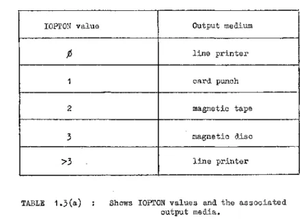
1. The user must specify the output medium for storage of the target
language. This is done by specifying a value for the variable IOPTON.
The value must be provided in G-12 format. Table 1.3(a) shows the
I0FT0N value Output medium
line printer
1 card punch
2 magnetic tape
3 magnetic disc
>3 line printer
TABLE 1.3(a) : Shows I0PT0N values and the associated output media.
2. The user must supply a list of all the variables in his routine(s)
which are non-scalar at their first occurrence. An indication must also
be given of whether the variables are literal or numeric. The reason for
this requirement is as follows. Suppose a non-scalar variable name is
used as an AFL function parameter. The type of the variable may not be
made apparent inside the function body. The parameter may therefore be
treated as a scalar (and incorrect code generated) unless the user explic
itly declares it to be non-scalar.
The number of non-scalar variables being declared is first provided
in 16 format. This is followed by a list of variable names in the format
of Diagram 1.3(a). The zero indicates that no additional dimension or
bound information has been supplied. The list is scanned and, corresponding
to each non-scalar variable name encountered, code is generated to set up an
entry in the dope vector table DOPES at run-time of the converted routine(s).
column
21 I
26
Array name blank
T i . * for numeric variable column “ 1 for literal variable
27
Diagram 1.3(a) : Shows essential information for non-scalars.
Initially, only one bloclc of space is allocated for each non-scalar
variable in the above list. This amount is increased or decreased as
required during the running of the converted program. At this stage
entries are set up in NAMES for all variable names appearing in the above
list.
There are two cases in which an entry of the above form should not
be supplied for a non-scalar variable. These are:
(i) If additional information is supplied, the entry will have instead
one of the forms described in §1.4 •
(ii) If a variable is scalar initially and becomes non-scalar later, no
entry of the above form should be supplied.
If no further information is provided for non-scalars, a certain amount
•of interpretation is essential. For example, to access an array element,
a chain of 23T0RE elements must first be interpreted. If additional
contiguous blacks of YSTORE, thus reducing the amount of interpretation
required.
Obviously, from the point of view of the execution time of the
converted program, it is better to provide as much additional information
as possible.
1.4- Additional Input Options
As discussed previously, it is to the user's advantage to supply as
much information as possible regarding his non-scalar variables. The user
may be able to supply full dimension and bound information for certain non
scalar variables at conversion time. Eor other non-scalar variables,
however, he may only know the number of dimensions at this stage. It is
possible that he will be able to supply the bounds for these variables at
run-time of the converted routine(s).
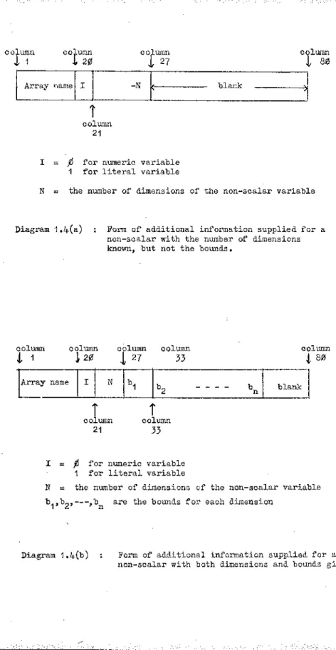
Two additional input options are therefore available to the user. He
can supply
1. the number of dimensions of a non-scalar variable with bounds' for each
dimension to be read in at run-time,
2. the number of dimensions of a non-scalar variable with fixed bounds
for each dimension.
The information corresponding to forms (1) and (2) above should be provided
in the format of Diagrams 1.4(a) and 1.4(b) respectively.
"When bounds and dimensions a r e 'specified, these are assumed to be the
fflavimum bounds for the array during running of the converted routine.
Thus the maximum number of elements of the array is known. The number of
23
CO.
J
.umn co. .umn , 201
lumnt 2 7
° 5
Array name I -N .... V
t column
2 1
I = ft for numeric variable 1 for literal variable
N = the number of dimensions of the non-scalar variable
Diagram 1.4(a) : Form of additional information supplied for a non-scalar with the number of dimensions known, but not the bounds.
column column column column column
i 1 i 20 J, 27 33 i 80
Array name I N
b 1 b0 --- b blank
2 n
t T
column column
21 33
I = j6 for numeric variable 1 for literal variable
N = the number of dimensions of the non-scalar variable
are the bounds for each dimension 1* 2* * n
parts of the dope vector entry.
If full information is provided, the non-scalar can he stored in
contiguous blocks of YSTORE. This eliminates the need for the time-
consuming access method used in the function FIND. The allocation of
contiguous blocks of YSTORE could have been arranged at the time when
initial information was processed. However, this would involve the
insertion of an extra test in FIND. More time would thus have been
required to access non-scalars for which no additional information was
supplied. This is best avoided. A call of the function FIND is there
fore produced for all non-scalar references and, where possible, this is
replaced by a simpler accessing function as an optimisation process.
Storage of certain non-scalars in contiguous blocks of YSTORE is
arranged in a pre-optimisation phase. It is done first for those arrays
with full information given. With the bound information supplied at run
time of the converted routine(s), (i.e. after optimisation proper), the
same process can be applied for non-scalars with only partial information
supplied initially.
The following path is therefore taken.
(i) Read in initial information, process, store until (iii), set up NAMES
entries and produce code to set up (partial) entries in D0EE3.
(ii) Convert routine(s) to target language with FIND calls for every non
scalar reference.
(iii) Carry out pre-optimisation phase in which storage is arranged in
contiguous blocks of YSTORE for those non-scalars with full inform
ation supplied.
(iv) Obtain bound information for the relevant non-scalars. Arrange these
(v) Replace RIND calls by simpler accessing function calls for all
non-scalars with more than the minimum amount of information
supplied. '
(vi) Optimise the generated code.
(vii) Run the converted program.
Stages (iii) and (v) are discussed in Chapter VII. Stage (vi) is
described in Chapter VIII.
At this stage an entry is set up in NAMES corresponding to each non
scalar variable name, and code is generated to produce partially filled
dope vector entries. The rest of the information supplied is stored
until required during the pre-optimisation phase.
The information temporarily stored at this stage is:
(i) the position of' the non-scalar variable name in the initial list,
(ii) the index of the non-scalar in NAMES,
(iii) the dimension and bound information in its original form.
The first stage of the conversion proper is a lexical scanning phase,
which is discussed in Chapter II.
The order of submission of information for the translation routines
is given below.
1. I0PT0N value (512 format)
2. Number of non-scalar variables, N (l6 format)
3. N cards with information as described in §1.3 and § 1.4 •
A. APL routine(s) to be converted
5. Blank card, signifying end of input.
CHAPTER II
LEXICAL SCANNING- PHASE
An APL routine first undergoes a lexical scan. Each line of the
routine is processed as described below, and the relevant information is
stored temporarily on tape.
This scanning,phase was initially introduced so that niladic function
calls would be recognisable as such during subsequent processing. Eor
example, consider the following routines:
V E < - A EN B j X
» i t
X <— E + A
i i
»
V
V E
F
i t i
V
During processing of function EN, it is not known that E is a niladic
function. This information only becomes available ’when the second function
definition is encountered. Since the code generated depends on the types
of all identifiers, it is necessary to scan each line in turn before the
main lino-by-3ine processing is carried out. This eliminates errors
resulting from incorrect types being associated with identifiers.
The lexical scanning phase is generally useful as it simplifies the
right-to-left scanning phase, which is discussed in detail in Chapter III.
The actions of the lexical scanning phase may be summarised as follows:
(i) All blank characters are removed.
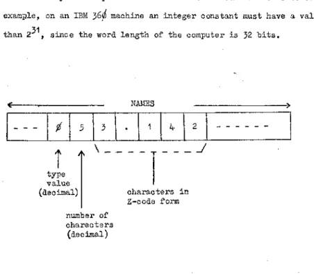
(ii) When an identifier name is encountered for the first time, an entry
is set up in the character array NAMES. The form of such entries
for different identifier types is described in §2.2 . Thereafter
all identifier names are replaced by the appropriate index in the
array NAMES.
(iii) All other symbols not comprising identifier names are replaced by
an integer value. Distinction is made at this stage between
monadic and dyadic uses of particular symbols.
Each line of the APL code is scanned from left to right. Tests are
first made for occurrences of the following symbols:
(i) the lamp-comment symbol
(ii) the 'del1 symbol .
The actions carried out on recognition of these symbols are described in
§2.11 and §2.12 respectively.
A test is then made for the occurrence of a symbol which can start an
identifier name. When such a symbol is met, each character in turn of the
identifier name is stored temporarily. After a complete identifier name
has been decoded, the array NAMES is accessed. The method of accessing
NAMES is also discussed in §2.2 . If no entry already exists in NAMES
for the identifier name, a new entry is added to the end of NAMES.
The processed APL line is stored in the character array NOLINE.
Corresponding to each identifier name, a 2-byte entry is added to NOLINE.
The entry represents the NAMES index for the identifier name. NAMES has
locations and, therefore, two bytes are sufficient to store the index
for any identifier name.
A single entry is set up in NAMES corresponding to constant vectors,
for example 3 4 5 in
X < ? - 3 A 5
Constant vector NAMES entries are discussed more fully in §2.10 .
The handling of other symbols is less straightforward. All symbols
are distinguished initially with the aid of a symbol table, which is
discussed in §2.1 .
The symbol table is arranged such that all dyadic operators are
grouped together at one end, and all monadic operators are grouped later,
with symbols which can be either monadic or dyadic appearing between.
Letters, digits and special symbols follow the above three groups. Thus
the address of a symbol in the symbol table can be used to determine the
group to which the symbol belongs.
APL operators are later handled by the expansion of macros, as
described in Chapter V. In general there is one macro for each operator,
although a few operators (for example, +, -, x ,t- , *) are grouped together and dealt with using a single macro expansion.
One method of handling each operator would be to replace the operator
by a macro name and maintain a set of pointers giving the start address of
each macro body. A more efficient method is employed here. Each operator
has an associated macro number (not a name). The macro number is used to
access a table, MCADDR, where the start addresses of the macro bodies are
gives the start address of the macro body for ’+' .
The above method eliminates the necessity to store a number of macro
names in a table.
Operators are replaced in NOLINE by a 1-byte entry representing the
required macro number. In fact, the entry gives the negative of the macro
number, so that identifier and operator entries can be distinguished,
(The second byte of an identifier entry may have a 1 in its left-most
bit position (and thus be negative} but it will always be preceded by a
a pr positive entry. NAMES indices must be <5 0 0 0> which is < 2 . There
fore the first part of an identifier entry will be positive.)
Identifier entries are stored in NOLINE with the two parts reversed,
the reason being that the- right-most (positive) part will be encountered
first in the subsequent right-to-left scan.
Monadic and dyadic uses of the same operator are detected during- this
scan and the appropriate entries are generated in NOLINE. This is based
largely on the fact that, if an operatox- is used in the dyadic sense, it
will be preceded by an identifier or ) or ~2 .
A similar test is used to distinguish the use of the symbol ’/' in
u/v (where u is a logical vector) and f/x (where f is a dyadic
operator) . Two different entries are set up in NOLINE corresponding to
'/' in the above expressions. Similarly for the symbol .
Distinction is also made between the symbols 1 D ’ and 1 Q 1 used
for input or output purposes. If these symbols are used for output, they
always precede a left specification arrow. A test is made for this
occurrence. If the test is satisfied, then an entry is set up in NOLINE
for * □ » or • O ' , but not xor the left specification arrow. Thus,
is then regarded as the monadic operator Q operating on A .
If the test is not satisfied, then an input use of the symbols is
intended. A different entry for □ or □ would be set up in N0LIN3
for this case.
The symbol is also used in a variety of circumstances. It can
appear in
(i) a constant identifier name
(ii) an inner product
(iii) an outer product
The three uses are distinguished at this stage. In the case of outer
products no entry is placed in NOLINE corresponding to the symbol '•* .
The preceding symbol 'o1 is sufficient to distinguish the occurrence of
an outer product.
All the other symbols are replaced in NOLINE by an entry giving the
negative of the appropriate macro number.
A table of information on APL symbols is given in Appendix 2. The
method of distinguishing all the APL symbols is discussed in §2.1 .
Several values are stored on tape, together with NOLINE. These are
values which are required in subsequent scanning phases. They include
NOLPTR, which gives the number of entries in NOLINE for a particular APL
line. Others are IFUNCT, IEXP and U N I , whose functions are described
2• 1 The Symbol Table and Its Method, of Access
Symbols are first obtained in Z-code form. However, similar sets of
symbols (suoh as the dyadic operators) cannot be grouped conveniently
according to S-code values. For this reason, a symbol table is maintained
in which convenient sets of symbols are grouped together.
The symbol table is a one-dimensional array ISYMBT 160 characters
in length. It contains the Z-code representations of all the legal
symbols in the APL language.
Y/hen a symbol is decoded a function is performed on the Z-code value.
This produces the first address, I, to be accessed in ISYMBT. If the
decoded symbol value equals ISYMBT (i), then the variable NADDR is set to
I. Otherwise successive addresses of ISYMBT are accessed, starting from
I ,until there is a match. The correct address is then stored in NADDR.
Operators can be:
(i) dyadic
(ii) monadic
(iii) dyadic or monadic .
The group to which a particular operator belongs can be determined
from the value of NADDR, for example:
(a) NADDR = 1 - 2 0 for purely dyadic operators
(b) NADDR = 2 1 - 3 8 for operators which can be either monadic or dyadic
(c) NADDR = 3 9 - 4 3 for purely monadic operators
In addition, the following groups can be distinguished.:
(d) NADDR = 44 - 52 for delimiters
(e) NADI® = 5 3 - 1 2 0 for symbols which can start identifier names
(letters, A , A, digits, decimal point, overbar,
•(high minus)-, blank and quote)
(f) NADDR = 121 - 123 for remaining symbols (colon, del and locked del).
Within each of the groups (a) to (f), symbols appear in the symbol table in
increasing order of Z-code value.
^•2 Identifier Names and the NAMES Table
A copy of all identifier names encountered is stored in the array
NAMES. The identifier name is thereafter replaced by the appropriate
index in NAMES. The characters comprising identifier names can thus be
re-accessed when required during the code production stage.
Identifier names must start with characters of the following types:
(i) a letter or a digit
(ii) a letter understruck
(iii) the characters 1A * or 'A'
(iv) the characters or *
If any of these symbols is decoded, successive characters comprising
the identifier name are stored in NAME, a 300-byte array. lor literal
identifiers, the enclosing quotes are first removed and double quotes inside
the string are replaced by single quotes.
The elements of a constant vector are stored in NAMES with a blank
character separating each element. A blank character also terminates
each constant vector.
When the entire identifier has been decoded, the non-zero characters
of the same length and type. This process is repeated until either
(a) a blank entry is reached in NAMES, or
Cb) a match is found between a NAMES entry and the contents of NAME.
The occurrence of (a) signifies that this is the first time the
identifier name has appeared in the APL routine. A new entry is then
set up in NAMES for the identifier. The form of the NAMES entry is given
in Diagram 2.2(a). (The type of the blank entry reached should be tested
as an empty literal vector will have a blank in the relevant part of the
NAMES entry.)
The occurrence of (b) indicates that the identifier name has already
appeared in the routine. A previous occurrence of the identifier name
is only confirmed if the type of the entry in NAME equals that of the
entry in NAMES.
It can be assumed that all variable names start with the permitted
characters, since only working APL routines will be converted.
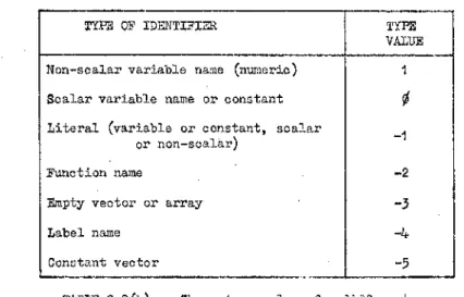
Table 2.2(b) gives the possible type values for all the identifier
types distinguished.
38
TYPE OF IDENTIFIER TYPE
VALUE
Non-scalar variable name (numeric) 1
Scalar variable name or constant
i
Literal (variable or constant, scalar
or non-scalar) - 1
Function name - 2
Empty vector or array - 3
Label name -K
Constant vector -5
TABLE 2.2(b) ; Shows type values for different types of identifier.