A shape memory alloy adaptive tuned vibration absorber: design and implementation

(1)

INSTITUTE OF SOUND AND VIBRATION RESEARCH

DYNAMICS GROUP

Design of an adaptive vibration absorbers using shape memory alloy

by

E. Rustighi, M. J. Brennan and B. R. Mace

ISVR Technical Memorandum No. 920

September 2003

Authorized for issue by Prof. M. J. Brennan

Group Chairman

(2)

A well-established vibration control device is the tuned vibration absorber (TVA). Even though such a device may be have different shapes it acts like a spring-mass system. For simplicity, in this project a beam-like TVA is used.

One of the drawbacks of such a device, however, is that it can detune during operation because of changes in forcing frequency. To maintain its tuned condition a variable stiffness element is required so that the natural frequency of the absorber can be adjusted in real-time.

In this project a beam-like TVA has been realized using shape memory alloy (SMA). Such a material changes its mechanical properties with temperature. By varying the temperature of the beam the absorber can be tuned in order to maintain the vibration of the host structure to be very small.

(3)

Nomenclature

a Attenuation A Cross section

Ae Surface of heat exchange

As, Af Austenite start and finish temperature of transformation

CA, CM Stress coefficients of transformation hysteresis

cp Specific heat

d Diameter of the wire

D Elastic matrix and derivative constant of control algorithm dn Derivative of the error at n-th time step

E Young modulus

en Control error at n-th time step

F0 Amplitude of the exciting force

Fn Modal forces

H Estimate of the FRF

I Geometric moment of inertia of the cross section and intensity of current IAE Absolute value of the error

In Current at n-th time step

in Integral of the error at n-th time step

k1 Stiffness of the base structure

k2 Stiffness of the dynamic absorber

Kn Modal stiffness

kn Stiffness at n-th time step

L Length of the beam

m1 Mass of the machine (host structure)

m2 Mass of the dynamic absorber

Mn Modal masses

Ms, Mf Martensite start and finish temperature of transformation

mtot Total mass of the beam

P Proportional constant of control algorithm Q Heat flow

(6)

R Electrical resistance

rAjk, rDjk Modal constant

S Autospectrum and cross spectrum

t Time

Tn(t), zn(t) Modal coordinates

U Internal energy u Motion of the beam

V Velocity amplitude and volume

X1 Amplitude of the displacement response of the machine

X2 Amplitude of the displacement response of the dynamic absorber

YR Modulus of rupture

YS Yield stress

z Displacement of a beam perpendicular to his axis z1 Point impedance of the machine

z2 Point impedance of the dynamic absorber

Zn(z) Mode shapes or stationary waves

∆H Latent heat of transformation Θ Thermo-elastic tensor

Ω Transformation tensor α Convective coefficient α(ω) Receptance

β Current constant

χ, ν Constants defined in the report

φ Angle between the responses of the machine and of the absorber φn Mass-normalized mode shapes

φn Mass normalized mode shapes

η Loss factor µ Mean value θ Temperature

θa Ambient temperature

ρ Density

(7)

σ Stress

τ Time constant

ω Frequency of the excitation and of the response ωa Anti-resonance frequency

ωn Natural frequencies

ωr Resonance frequency

(8)

1. Introduction

A well-established vibration control device is the tuned vibration absorber (TVA), which can be used to suppress a troublesome resonance or to attenuate the vibration of a structure at a particular forcing frequency. Even though such a device may have different forms, it basically acts like a spring-mass system.

One of the drawbacks of such a device, however, is that it can detune during operation because of changes in forcing frequency or the stiffness of the device could change. To maintain its tuned condition a variable stiffness element is required so that the natural frequency of the absorber can be adjusted in real-time [1]. This can be achieved in a number of ways for example by altering the pressure in a set of rubber bellows [2], altering the gap between two beams forming a compound cantilever beam [3], adjusting the number of active coils in a coil spring [4] or changing the temperature of a viscoelastic element [5].

The main advantage of an actively tuned device is that low damping can be used if the tuning is precise and this reduces the need for a large mass [1]. In order to automatically tune the vibration absorber, a control strategy can be used, such as that proposed by Long et al [2] or Kidner and Brennan [6-8].

Semi active control operates by generating a secondary force passively, by actively altering the characteristics of the system, so the passive system is most effective. Semi active devices can attain high reductions in the level of vibration and only require modest amounts of power for the sensors and the controller. By not putting energy into the system (apart from small amounts to tune the system), semi active devices are generally less expensive and inherently more stable than their fully active counterparts. Vibration control systems illustrated in the literature have been tuned using feedforward and feedback controls or various adaptive strategies.

(9)

The main limitations of SMAs are the slow response time (bandwidth is limited due to heating and cooling restrictions and can only achieve a few Hz at the very best) and the poor energy conversion efficiency when actuated with an electrical signal [9-11]. A brass TVA and a SMA TVA have been built and experimentally characterised. The results show the feasibility of using SMA properties to tune such a device. At the same time the numerical analysis shows the effectiveness and robustness of a simple non linear adaptive system that considers only the phase between two signals measured from the TVA.

As it is planned to implement an automatic adaptive control system a numerical analysis is carried out in parallel with the experimental one. The aim is to make a brief comparison of adaptive systems possible for tuning the stiffness of a dynamic vibration absorber and then to discuss in detail a control system for the SMA TVA.

(10)

2. Tunable vibration absorber (TVA)

2.1. Introduction

This section outlines the principle of a TVA and describes a particular configuration in which it could be designed. The first part of the section deals with the theoretical modelling of a TVA and shows the main equations necessary to describe its behaviour. The second part of the section introduces the guidelines to design a beam as a TVA. A 2dof model is introduced to simplify the complex continuous model of the beam.

2.2. Classical and advanced theory

A machine may experience excessive vibrations when excited by a force whose excitation frequency nearly coincides with a natural frequency of the machine. In order to reduce the vibration level a vibration absorber may be used. This is simply an additional spring-mass-damper system that is added to the machine so that the natural frequencies of the resulting system are away from the excitation frequency and, ideally, there is an antiresonance at the excitation frequency.

This absorber is actually designed in two distinct ways: the first is when it is tuned to a problematic resonance of the host structure and the other is where it is tuned to a troublesome excitation frequency. In the first case the purpose of the absorber is to add damping to reduce the motion of the structure at frequencies close to the resonance frequency (broadband effectiveness). In the second case its purpose is to add a large mechanical impedance to the host structure at a single frequency of excitation with the aim of minimizing the motion of the structure at this frequency (discrete frequency effectiveness) [1]. It is the second case that is the subject of this work, and the device is usually called a tuned vibration neutralizer (TVN) or a tuned vibration absorber (TVA). The analysis of a vibration neutralizer is considered by idealizing the machine to which it is attached as a single degree of freedom system as shown in Figure 1. When a harmonic force F0eiωt acts on the machine the amplitudes X1 and X2 of the masses are

given by

(

)

(

2 ₂

)

₂ 0

2 1

2

0 2 2 1 2 1 2 1

= +

− + −

= −

+ + −

X k m X

k

F X k X k k m

ω ω

(11)

Rearranging equations 1a and 1b gives the steady state displacement amplitudes of the two masses m1 and m2:

(

)

(

)(

)

(

)(

)

2

2 2 2 2 2 1 2 1 2 0 2 2 2 2 2 2 2 1 2 1 2 2 2 0 1 k k m k k m k F X k k m k k m m k F X − + − + + − = − + − + + − − = ω ω ω ω ω (2a,b)

It is clear from equation 2a that in order to reduce the vibration of the machine the natural frequency of the neutralizer must be the same as the excitation frequency, i.e.

2 2

2 ₌ω

m k

(3) Equations 2a and 2b can be simplified by assuming the machine vibrates like a simple

mass (i.e. k₁ =0). Such simplification is reasonable because often m1 is on soft springs

for vibration isolation and the excitation frequency is much greater than the machine resonance frequency. Moreover, if we now consider the structural damping of the neutralizer, so that k₂ ≡k₂

(

1+iη

)

, we obtain

(

)

(

)

(

)

(

)

2 0

2 2 1 2 2 1 4 2 1 2 2 2 0 2 2 2 1 2 2 2 1 4 2 1 2 2 2 2 1 F k m m i k m m m m ik k X F k m m i k m m m m ik m k X

aω ω η

ω η η ω ω ω η ω + − + − − − = + − + − + − = (4a,b)

The amplitudes are given by

(

)

(

)

(

)

(

)

(

)

(

)

(

)

2

(

2

)

2 2 2 1 6 2 2 1 2 1 8 2 2 2 1 2 2 2 0 2 2 2 2 2 2 1 6 2 2 1 2 1 8 2 2 2 1 2 2 2 2 2 2 2 4 2 2 0 1 1 2 1 1 2 1 2 η ω ω η η ω ω η ω ω + + + + − + = + + + + − + + − = k m m k m m m m m m k F X k m m k m m m m m m k k m m F X

and the phases are

(

)

(

)

( )

(

₍

)

₎

_      + − + − − = ∠       + − + − −       − = ∠ 2 2 2 1 4 2 1 2 2 2 1 2 2 2 2 1 4 2 1 2 2 2 1 2 2 2 2 1 arctan arctan arctan arctan ω ω η ω η ω ω η ω ω η k m m m m k m m X k m m m m k m m m k k X

If we consider the difference of phases we obtain

( )

η

ω η

φ arctan ₂ arctan

2 2

1 −

(12)

(

)

( )

_{( ) ( )}

( )

β α β α β α tan tan 1 tan tan tan + − = −

it follows that

( )

₍

₎

₂

2 2 2 2 2 1 tan ω η η ω φ m k m − + =

The difference of phase φ is also physically comprised between 180° and 360°, as can be inferred from equations 4a and 4b, and therefore

( )

_{( )}

[

( )

]

(

)

2 2 2 2 2 2 2 2 1 1 1 tan Sign tan 1 1 cos       − + + ± = + − = ω η η ω φ φ φ m k

m (5)

This equation is useful because the goal is to tune the TVA so that ω = k₂ m₂

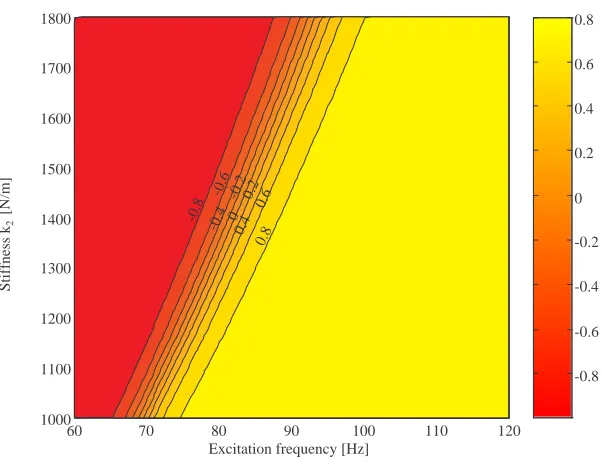
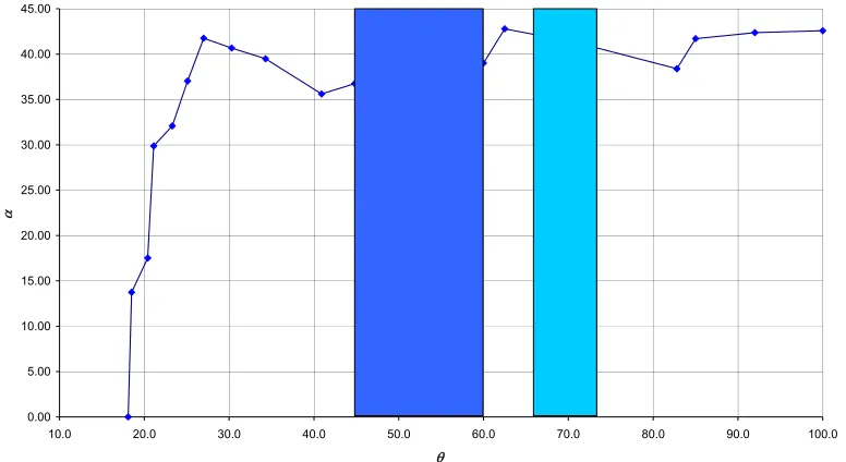
(equation 3) and the tuning strategy is to use the cosine of the phase difference between the measured responses X1 and X2 as an error signal. In order to tune the neutralizer to

the excitation we plan to change its stiffness so that cos

( )

φ =0. Figures 2-5 show various relations between stiffness, cos

( )

φ and the excitation frequency.

It is convenient to write down the governing equations of motion of the machine and the neutralizer in the frequency domain in terms of their mechanical impedances (see [12]), which are given by [13]

2 2 2 1 1 1 m k j z m j z ω ω ω − − = =

Figure 6 depicts an impedance diagram of the system.

Given that the two sub-systems are in parallel, the impedance of the resulting system is

(

)

[

]

2 2 2 2 1 2 2 2 1 2 1 k m m m k m m j z z z − + − = + = ω ω ω (6) Figure 7 shows the impedance as a function of frequency. Referring to the total system,

there is a resonance, ωr, when the numerator is zero (the impedance is zero, that is a

null force could move the system) and there is an anti-resonance, ωa, when the

(13)

(

)

2 1 2 1 2 2 2 m m m m k m k r a + = = ω ω (7a,b)

The anti-resonance frequency of the system, ωa, coincides with the resonance of the

TVA, in fact the machine doesn’t move and behave as if it were grounded.

Note that the anti-resonance coincides with the resonance of the neutralizer (in accordance with equation 3) because the mass of the machine is constrained to have zero motion.

Brennan [1] showed that that the displacement of the machine can only be reduced significantly if the impedance of the neutralizer is much greater than that of the machine. The effectiveness of the neutralizer may be judged by the amount that it attenuates the displacement of the machine to which is attached, so we define the attenuation as the ratio of the free motion of the machine to the motion of the machine with the neutralizer fitted. Assuming that the impedance of the neutralizer is much greater than the impedance of the machine (neutralizer properly tuned), the attenuation has the following form

2 1 1 2 z z z a z

>> ≅ (8)

If the neutralizer is tuned to the excitation frequency and assuming that η<<1 then the impedance of the vibration neutralizer is approximately given by

η ω η ω ω 2 1 2 m z a a ≅

<<= (9)

and the attenuation by

2 1 2 1 1 2 1 m m m m z z a a a η η ωω

ηω ω

= ≅

<<=

(10)

Equation 9 shows that the impedance of the neutralizer 1. increases with frequency;

2. increases with the mass; 3. decreases with damping.

(14)

The half power bandwidth over which the vibration of the machine is reduced is proportional to damping in the neutralizer and is independent of the mass ratio, so the only way of achieving a large attenuation without sacrificing bandwidth is to increase the mass ratio.

2.3. The free-free beam as a TVA

A very simple neutralizer can be obtained by attaching a beam to the host structure in its centre. For frequencies around the first natural frequency of the beam, it behaves essentially as a sdof system. Using such a configuration it is possible to use shape memory alloy wires in a straightforward way.

First the lateral vibration behaviour of a free-free beam is considered. The equation of motion of the beam is

( )

2 4 2

2 _, _,

z t z u EI t

t z u A

∂ ∂ − = ∂ ∂

ρ (11)

where ρ and A are the density and the cross section of the beam and u is the lateral displacement of the beam and is a function of the time t and of the axial coordinate z. E and I are the Young modulus and the second moment of area of the cross section. The solution of the equation can be found using the method of separation of variables writing

( )

z,t Z(z)T(t)

u = equation 11 can now be written as

Z Z T

T IIII

2

ν − =

where

A EI ρ ν =

(·)IIII is the fourth derivative with respect to the axial coordinate z.

The left hand side depends only on time t and the right hand side only on the displacement z so the two sides must be both equal to the same constant. Thus we obtain the following equations

0 0

2 2

2

= −

= +

Z Z

T T

IIII _ω

ν ω

(15)

z F z E z D z C Z t B t A T χ χ χ χ ω ω sinh cosh sin cos sin cos + + + = + = where ν ω χ =

Considering the boundary conditions for a free-free beam we have

( )

Z

( )

Z

( )

L Z

( )

L

ZII ₀ ₌ III ₀ ₌ II ₌ III

where (·)II and (·)III are the second and third derivative with respect to the axial coordinate z.

Applying these boundary condition leads to the following equation:

(

)

(

)

(

sin sinh

)

(

cos cosh

)

0

0 sinh sin cosh cos = − + + − = − + − = = L L D L L C L L D L L C F D E C χ χ χ χ χ χ χ χ

In order for these to be a non-trivial solution we obtain 1 cosh cosχL⋅ χL=

Several solutions of this equation for χ, are given in Table 1. Note that also χ=0 is a solution, and represents the rigid motion of the undeformed beam. Actually there are two solutions for χ=0 that represent the translational and rotational motion. As in this work we are dealing with a beam supported in the centre, the rotational rigid body motion is neglected.

The natural frequencies of the system are given by

2

n

n νχ

ω = and expressing the constant D in terms of C gives

L L L L C D n n n n n

n _χ _χ

χ χ cosh cos sinh sin − + =

The solution for the displacement can therefore be written as

      + + + = z C D z z C D z C Z _n n n n n n n n n

n cosχ sinχ coshχ sinhχ

The correct value of the constant C is found from boundary conditions.

(16)

j i z Z AZ L j

i = ∀ ≠

∫

d 0

0

ρ

In the same manner we could express the stiffness orthogonality condition as j i z z Z z Z EI L j

i ₌ _∀ _≠

∫

d 0

d d d d 0 2 2 2 2

Using the orthogonality properties of mode shapes, it is possible to develop a modal superposition procedure for distributed parameter systems. As is the case for discrete systems, the displacement solution is expressed in terms of a linear combination of mode shapes as:

( )

_∑

( ) ( )

_∑

∞

( ) ( )

= ∞ = ⋅ = ⋅ = 0 0 ,

i i i

t z z Z t T z Z t z

u (12)

Substituting this in to equation 11, to which the distributed force q has been added, multiplying both sides by the mode shape Zj, integrating and applying the orthogonality properties we get the following system of uncoupled modal equations:

( )

= ∞ =       + ∂ ∂

∫

d

∫

, d 0, ,

d d 0 0 4 4 2 2

2 _z _z _Z _q _z _t _z _n _…

z Z EIZ t z AZ L L n n n n n n ρ

These equations can be written in a simpler form by introducing the following definitions:

Modal mass: M_n =

∫

L AZ_n z

0

2_d

ρ

Modal stiffness:

∫

_

     ≡

=L n L n

n n z z Z EI z z Z EIZ K 0 0 2 2 2 4 4 d d d d d d

Modal force: F_n

( )

t =

∫

LZ_nq

( )

z t z

0

d ,

The equation for the n-th mode thus becomes

n z n z

nz K z F

M + =

This is the same expression that is obtained with the Rayleigh method applied for continuous systems. Solutions of each modal equation can be now obtained straightforwardly.

(17)

The receptance can be written in terms of the modal properties as

( )

[

] [ ]

[

(

₂ ₂

)

]

1

[ ]

T

φ ω ω φ ω

α = _n − −

or in the explicit formulation

( )

_∑

( )

_∑

₍

( )

₎

( )

= = − = − = = N

n n n

k n j n N n n k n j n k j k j M z Z z Z z z F X

0 2 2

, _ω _ω _ω _ω

φ φ ω

α .

Thus the point mobility (see [12]) at the centre (z=L/2) of a free-free beam is given by [6]

( )

_∑

∞

₍

(

₎

)

= − + = =

1 2 2

2 2 / , 2 / 2 / 2

/ 1 /2

n n n tot L L L

L i L

m i i F V ω ω ωφ ω ω ωα

in which the first term is the mobility of the translational rigid motion. The rotational rigid motion is missing because of the symmetry around the excitation point.

Considering only the first mode of vibration besides the rigid body motion

(

)

(

2 2

)

1 2 1 2 / 2

/ 1 /2

ω ω ωφ

ω + −

≈ i L

m i F V tot L

L ₍₁₃₎

The resonance is clearly at ω=ω1 and the anti-resonance is at

(

/2

)

1 ₁2

2 1 L m_tot a _φ ω ω +

= (14)

A two dof system (equation 7) consisting of two masses connected by a spring that fits this simplified model (equation 12) should have the following mass ratio [6]

(

/2

)

1.478

2 1 1

2 ₌_m _L ₌

m m

totφ

In summary, in order to approximate the behaviour of a free-free beam supported in the middle in a frequency range up to the first natural frequency or so, we can use a simplified two dof system with the following characteristics

tot tot tot tot m k m m m m m 2 1 2 1 478 . 2 596 . 0 596 . 0 404 . 0 478 . 2 ω ⋅ = ⋅ = ⋅ = = (15a,b,c)

2.4. Summary

(18)

(19)

Figures

Figure 1 Undamped vibration neutralizer fitted to an undamped single degree-of-freedom system (Machine)

60 70 80 90 100 110 120

1000 1100 1200 1300 1400 1500 1600 1700 1800

Excitation frequency [Hz]

Stiffness k

2

[N/m] _-0.8

-0.6

-0.4 -0.2 0

0.2

0.4 0.6

0.8

[image:19.595.140.441.314.546.2]

-0.8 -0.6 -0.4 -0.2 0 0.2 0.4 0.6 0.8

Figure 2 Variation of the cosine of the phase difference vs. excitation frequency and stiffness (m1=0.0036 kg; m2=0.0053 kg; η=0.1)

m1

m2

k2

k1

Neutralizer

Machine F0eiω t

X1

(20)

60 70 80 90 100 110 120 -1

-0.8 -0.6 -0.4 -0.2 0 0.2 0.4 0.6 0.8 1

cos

φ _k = 1.5 N/m2 k

[image:20.595.141.459.385.630.2]

2 = 2 N/m k = 1 N/m2

Figure 3 The cosine of the phase difference vs. excitation frequency at different stiffness values (m1=0.0036 kg; m2=0.0053 kg; η=0.1)

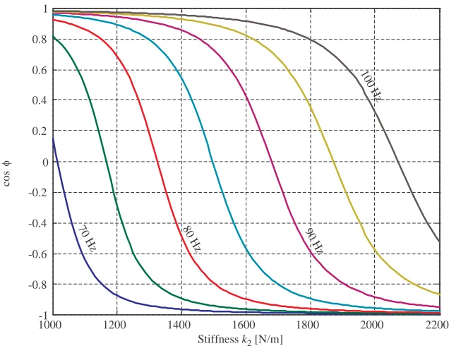
1000-1 1200 1400 1600 1800 2000 2200

-0.8 -0.6 -0.4 -0.2 0 0.2 0.4 0.6 0.8 1

Stiffness k₂ [N/m]

cos

φ

70 Hz 80 Hz 90 Hz

100 Hz

(21)

0 50 100 150 0

500 1000 1500 2000 2500 3000 3500 4000 4500 5000

Stiffness

k2

(when cos

φ=0) [N/m]

Figure 5 The tuned value of the neutralizer stiffness vs. the excitation frequency (m1=0.0036 kg; m2=0.0053 kg; η=0.1)

Figure 6 Impedance schematization of the vibration neutralizer.

m1

k2

m2

F

V

m1

m2

k2

(22)

101 102 101

102 103 104 105

Frequency [Hz] F

orce /V el ocit y [N s ec/m ]

101 102

-100 -50 0 50 100

Frequency [Hz] P

hase a n gle [d e gree ]

Figure 7 Impedance of a system comprising a mass and a neutralizer (m1=5 kg; m2=1 kg; k2=63165 N/m; η=0.01)

Tables

n 1 2 3 4 5

χnL 4.730 7.853 10.996 14.137 π

     + ≈

2 1 n

(23)

3. Shape Memory Alloys

3.1. Introduction

This section introduces the properties of SMA. The mathematical models used to describe such properties are discussed in order to present the tools to design a mechanical structure involving their use. Since the TVA, described in this report, involves the temperature control of SMA wire, a thermal model of such a system is developed. An electrical current will be used to input heat in the material and change the temperature of the wire so as to change its mechanical properties. A short review of the application of SMA as a smart material in controlled systems is also presented. Shape memory alloys are metals that have the property by which they can remember their original size and shape and revert to it at a characteristic transformation temperature. Generally, they can be plastically deformed at some relatively low temperature, and upon exposure to some higher temperature will return to their shape prior to the deformation. Materials that exhibit shape memory only upon heating are referred to as having a one way shape memory. Some materials also undergo a change in shape upon re-cooling, showing a so-called two way shape memory effect. The shape memory effect can be a one way or two way effect depending on the type of the material training1.

Although a relatively wide variety of alloys exhibit the shape memory effect, only those that can recover substantial amounts of strain or that generate significant force upon changing shape are of commercial interest. In such materials, heating and cooling could produce large mechanical deformation (thermomechanical strain is in the range of 5-10%). To date, this has been the nickel-titanium alloys and copper-base alloys such as CuZnAl and CuAlNi.

The first recorded observation of the shape memory transformation was by Chang and Read in 1932. They noted the reversibility of the transformation in AuCd by metallographic observations and resistivity changes. However, it was not until 1960, when Buehler and co-workers at the Naval Ordnance Laboratory discovered the effect

1_{MATERIAL TRAINING: Two-way shape memory behaviour is accomplished by introducing internal}

(24)

in equiatomic nickel-titanium (NiTi), that research into both the metallurgy and potential practical uses began in earnest. They named it NiTiNOL to include the acronym of the name of their laboratory. Study of shape memory alloys has continued at an increasing pace since then, and more products using these materials are coming to the market each year. For instance because of their biocompability and superior resistance to corrosion, shape memory alloys have gained wide usage in the medical field as bone plate, artificial joints, orthodontic devices, coronary angioplasty probes, arthroscopic instrumentation, etc. [10, 14, 15]

Following this introduction, the next section outlines the properties of the SMA and deals with the thermo-mechanical models that can be used to describe the behaviour of the material. Besides a complex tri-dimensional constitutive model, a simplified model appropriate for SMA wires, is described. The third subsection describes the thermal behaviour of a SMA wire, as the main objective of this report is to control the temperature of a SMA wire acting as a TVA. The fourth subsection outlines the properties of the SMA wire used to build the TVA described in this report. The SMA properties given by the company and those observed in the experiments are compared. The fifth subsection summarizes some applications of SMA in control devices and a summary subsection ends the section.

3.2. Phase transformation: shape memory effect and

superelasticity

3.2.1. Crystallography of martensite and austenite

The shape memory effect is related to the molecular structure of the material, i.e. SMA materials undergo a phase transformation when heated or cooled. The phase change is between two solid phases and involves rearrangement of atoms within the crystal lattice. The internal structure is different at different temperatures. The low temperature phase is known as martensite, with highly twinned crystalline structure, and the high temperature phase is called austenite, with a body-centered cubic structure (see Figure 9).

(25)

material with its corresponding grain boundaries. The martensite grains form a heavily twinned structure, meaning they are oriented symmetrically across grain boundaries. The twinned structure allows the internal lattice of individual grains to change while still maintaining the same interface with adjacent grains. As a result, SMA can experience large macroscopic deformations while maintaining remarkable order within its microscopic structure.

3.2.2. Hysteresis loop – model of transformation

The difference between the transition temperatures upon heating and cooling is called hysteresis. Hysteresis is generally defined as the difference between the temperatures at which the material is 50 % transformed to austenite upon heating and 50 % transformed to martensite upon cooling. This difference can be up to 20-30 °C.

The phase transformation model has five parameters: the fraction of martensite in the material ξ; the temperature at which austenite phase transformation starts and finishes, As and Af; the temperature at which martensite phase transformation starts and finishes, Ms and Mf. Material tests reveal that the relationship between martensitic fraction ξ and temperature θ takes the form shown in Figure 10 [10, 16, 17]. During a full transformation the functions ξM→A(θ), from the martensite to the austenite state, and the function ξM←A(θ), from the austenite to the martensite state, are similar to a cosine function given by

       > ≤ ≤ = +         − − < = _→ → f f s A M s f s s A M A A A C A A A A θ θ θ π θ ξ 0 2 1 cos 2 1 1 (16)        > ≤ ≤ = +         − − < = _← ← s s f A M f s f f A M M M M C M M M M θ θ θ π θ ξ 0 2 1 cos 2 1 1 (17)

During a partial transformation the function of the martensite ξˆ_M_→_A

( )

θ and ξˆ_M_←_A

( )

θ are given by

A M MA A

M→ =E ξ →

ξˆ ₍₁₈₎

(

)

[

AM M A

]

AM

A

M← = −E ξ ← +E

(26)

where EMA and EAM are the amplitude of these functions that change depending on the

history of the deformation and must be updated when there is a change in the gradient of temperature in accordance with

       > ≤ ≤ < = ← → ← ← f A M f s A M A M s A M MA A A A C A E θ ξ θ ξ θ ξ ˆ ˆ ˆ (20)        > ≤ ≤ − − < = → ← ← → → s A M s f A M A M A M f A M AM M M M C C M E θ ξ θ ξ θ ξ ˆ 1 ˆ ˆ (21)

The transformation temperatures are also functions of stress: these parameters increase with an increase in tensile stress. Thus, phase transformation can occur at constant temperature by applying stress to the SMA. Increasing the stress increases the temperature associated with the phase transformation. So even if the temperature is constant, the fraction of martensite increases due to the increase in the applied stress. Experiments demonstrate that the critical temperatures are a linear function of the applied stress.

Increasing the stress results in a shift towards the martensitic phase and away from the austenitic phase. A simple rule to remember is that increasing the stress is equivalent

to decreasing the temperature. These effects can be modelled by incorporating an

equivalent temperature into the equation

      − = − = → ← A eq A M M eq A M C C σ θ θ σ θ θ . . (22)

where CA=tan(α) and CM=tan(β) (see Figure 11). Usually α=β. 3.2.3. Constitutive model of SMA

(27)

The stress state in an SMA component is a function of three primary state variables. They are the fraction of martensite, the temperature at which the component is operating and the strain at which the component is functioning. Therefore

(

ε θ ξ

)

σ

σ = , , (23)

Here σ is the Piola-Kirchoff stress tensor and ε is the Green strain tensor [10, 16, 18] because SMA components are usually involved in large strain applications (strains of the order fo 10-1 rather than 10-6).

A constitutive expression can be obtained from the integration of the differential equation 23 with respect to time from the initial conditions ε₀, θ₀, ξ₀. Thus

(

0

)

(

0

)

(

0

)

0 ε ε θ θ ξ ξ

σ

σ − = D − +Θ − +Ω − (24)

where D is the elastic matrix, Θ is the thermo-elastic tensor and Ω is the transformation tensor.

However, the SMA device used in the work described in this report operates only in the elastic region and utilises just the change in the Young modulus.

3.2.4. Shape memory effect and superelasticity

The fundamental coupling mechanism in SMA materials is thermomechanical because the stress-strain behaviour is strongly linked to the phase of the material.

Supposing that it operates at a constant temperature, a simplified model could be made in order to explain the two main effects of SMA. In such a model a linear elastic behaviour is exhibited when ξ=1 or 0, but with different stiffness constants, whereas a large increase in strain occurs during the phase transformation. Thus, the stress strain response exhibits two linear elastic regions and a plateau with a large increase in strain (softening) during the phase change (see Figure 13-b in which letters help to follow the several steps; Figure 13-a maps the same steps in the martensite fraction plane). If we load the material when it is in the austenitic phase (step a) we induce the AÆM phase change (steps b to c) until reaching a total martensitic state (step d). Now, if we unload the material we induce a residual strain, i.e. a permanent deformation (see step e in Figure 13-b), because the MÆA phase transformation will not occur. Only upon heating the wire the martensitic residual strain may be recovered and the material reaches again the step a. This is called shape memory effect.

Starting with ξ=0 and θ>Af (step a of Figure 14) and loading the material, it reaches the

(28)

material it passes through the MÆA transformation (step e to f), we obtain another softening effect and the material exhibits a hysteresis loop. The area of the hysteresis loop (among the steps b-c-e-f) is equivalent to the amount of energy dissipated during the stress strain cycle. This behaviour is called superelastic effect.

A typical ductile material can absorb a large amount energy only when the stress becomes higher than the yield stress of the material so that it undergoes plastic deformation. This property is a problem because repeated loading will eventually cause failure (low cycle fatigue). On the contrary, SMA exhibits a superelastic stress-strain response that make SMA suitable for absorbing and dissipating energy: increasing the applied stress will cause what appears to be a yielding of the material, but reducing the stress back to zero results in zero strain.

3.2.5. Simplified mechanical relations

In the linear region the stress strain relationship is simply (E is the elastic modulus)

(

ε ε0

)

σ =E −

The amount of stress that occurs before the phase transformation depends on the initial temperature of the material and the values of CM and CA. At the limit of linear

behaviour the equivalent temperature equals the martensite start temperature MS (see

Figure 15-a,b) and

S M

eq _M

C =

−

= lim

. lim

σ θ θ

So at the temperature θ0 the linear elastic strain is

(

S

)

M M

C −

= ₀

lim θ

σ

The constitutive relationship during a phase transformation, assuming constant temperature, is equal to

(

ε ε0

)

(

ξ ξ0

)

σ =E − −ES_L −

where SL is the maximum strain recovery (see Figure 16-a,b), which is a property of the

material and is usually given for a particular material.

3.3. Thermal behaviour of a wire of SMA

(29)

The first law of thermodynamics states that the change in internal energy U of a system is equal to the heat added to the system minus the work done by the system. A simple wire does no work so the balance of energy is expressed by

U Q d d = where Q is heat flow through the system.

The variation of internal energy is related to the change in the temperature θ of the system by t Vc t U p d d d

d ₌_ρ θ

where ρ is the density, V is the volume and cp is the specific heat of the system.

If there are no sources of heat the temperature of the wire tends to the ambient temperature. The only heat exchange is convective dissipation for which the heat loss can be approximated by

( )

(

a

)

e t

A t

Q₌₋_α _θ ₋_θ d

d

where α is the convective coefficient and Ae represents the surface of heat exchange.

If the wire is heated by a current of intensity I the net heat input is expressed by

( )

(

a

)

e t

A R I t

Q ₌ 2 ₋_α _θ ₋_θ

d d

where the electrical resistance R of the wire is

A L R= ρ_e

setting ρe as the electrical resistivity and, L and A as the length and the cross section of

the wire.

So, when the wire cools down, it follows that

(

)

(

)

    = = − − = 0 0 d d θ θ θ θ α θ ρ t A t

Vc_p _e _a

Given the initial condition, the temperature is given by

( ) (

t θ θa

)

e t θa

θ ₌ ₋ − τ ₊

0 (25)

in which the time constant τ is

e p A Vc α ρ

τ = (26)

(30)

(

)

(

)

    = = − − = 0 2 0 d d θ θ θ θ α θ ρ t A R I t

Vc_p _e _a

whose solution, given the initial condition, is

( )

[

θ

(

θ β

)

]

(

θ β

)

θ ₌ ₋ ₊ −τ ₊ ₊

a t

a e

t ₀ (27)

in which the “current constant” β is defined as

e

A R I α

β = 2 (28)

This term represents the difference between the steady state “hot” temperature and the ambient temperature. In the limit of t→∞ equation 27 becomes

( )

θ β

θ ∞ = _a + (29)

For SMA devices, it is important also to consider the release and absorption of the latent heat of phase transformation, ∆H, which tends to slow down heating as well as cooling [19, 20]. When an electric current circulates in a SMA wire, its temperature increases according to the exponential equation. When the wire temperature reaches As

the material begins to absorb energy to sustain phase transformation. Once the phase transformation is over the temperature of the wire increases again in an exponential manner. In the same way, when the current is shut off the wire starts to cool down but at the temperature Ms the material begins to release the latent heat of transformation

until phase transformation is over.

Physically, during the phase transformation the internal energy of the wire is expressed by       ₋_∆ = t H t c V t U p d d d d d

d _ρ θ ξ

This equation is inconvenient because of the presence of the differential of the martensitic fraction. An estimate of the order of magnitude of the influence of the transformation on the response of the SMA wire can be formed by computing the time taken for the transformation to occur. Supposing the phase transformation is isothermal, the transformation time is given by

(

t a

)

e A R I H V t θ θ ξ ρ − − ∆ ∆ − = ∆ ₂

(31)

      → + → + = ation transform Austenite Martensite 2 ation transform Martensite Austenite 2 f s f s

t _A _A

M M θ

A physically realistic approximation of this process can be realized by approximating the experimental curve of the heat flow (see Figure 17) by a second order polynomial to model the change of specific heat during the phase transformation [20], i.e.

    + + = otherwise . transform phase during ˆ 2 p c d b a

c θ θ

The latent heat of transformation is calculated by integrating the specific heat with respect to temperature

∫

= ₋ − = s f f s M M f s A A s f c M M c A A

H 1 ˆdθ 1 ˆdθ

A rough approximation of this behaviour could be made by considering the specific heat during the phase transformation to take a different value which includes the latent heat of transformation. Moreover to avoid the problem due to the hysteresis we can pose a simple equation for the specific heat, namely

   > < ≤ ≤ ⋅ = f f p f f p A ;θ M θ c A θ M c e

cˆ (30)

Figure 18 shows the expected effect of such approximation.

The steady state temperature of the system when a current I is passed through the wire can be found from

( )

(

)

0

d

d ₌ 2 ₋ _∞ ₋ ₌

∞

= e a

t

A R I t

Q _α _θ _θ

The convective coefficient is given in terms of the steady state temperature as

( )

(

a

)

e A R I θ θ α − ∞

= 2 (31)

3.4. Nickel-Titanium alloys (Nitinol) properties

(32)

The company comments on this data as follows: “These values should only be used as guidelines for developing material specifications. Properties of Nitinol Alloys are strongly dependent on processing history and ambient temperature. The mechanical and shape memory properties shown here are typical for standard shape memory wire at room temperature tested in uniaxial (tensile) tension. Bending properties differ, and depend on specific geometries and applications. Modulus is dependent on temperature and strain. Certain shapes or product configurations may require custom specifications.”

The company also add to each sample the results of a free-recovery test in which are reported the measured temperatures of austenite transformation. Table 3 shows the results of such a test.

Table 4, extracted from different papers and books [9, 10, 14, 21], synthesizes the most important values necessary to make provision for the behaviour of a SMA component. For instance, from this table we can infer that the Young modulus should increase by 2-3 times from the martensite to the austenite state. However, the experimental results in this report described in subsection 5.2 showed that there were significant discrepancies between data provided by the company and the estimated values.

Table 5 shows the values used in the calculations to predict the behaviour of the Nitinol wire used in the project, that have showed a good agreement with the experimental tests. All the values cited have been measured except the latent heat of transformation because of the lack of the proper equipment (see section 5).

3.5. Achieving control structures using SMA

SMA devices have been publicised in many fields but, in engineering, these materials have been used mainly as force actuators. They also offer vibration control potential based on three important principles [11]: 1) the large increase in the elastic modulus in the transition from martensitic to austenitic phase; 2) the creation of internal stresses; 3) the dissipation of energy through inelastic hysteresis damping.

(33)

trigger an on-off controller with a controlled dead band. The control action was sent to two power amplifiers that energized the actuators to provide the control forces. The excitation was just a step imposed at the free end.

Moreover SMA could also be used to build an active tuned vibration absorber (ATVA). Liang and Rogers explored two different techniques for SMA in vibration control [9, 22, 23]. The first was active properties tuning (APT), where the change in the elastic modulus of SMA with heating was used to modify the dynamic characteristics of a composite plate in which the SMA wires had been embedded. The other technique was the active strain energy tuning (ASET). In that application, SMA elements were given initial plastic strains before insertion into a composite material. Heating the SMA then resulted in in-plane forces within the plate, with subsequent changes in the structure’s natural frequency and mode shapes.

In some applications it is not practical to redesign an entire structural system to apply this technique. An alternative approach is to use just the adaptive properties of SMA to realize an ATVA. An SMA spring element whose stiffness is directly dependent on the elastic modulus of the spring material can be constructed as the adaptive spring in an ATVA. Following the work of Liang and Rogers, Williams et al [9] designed and built an ATVA using spring elements composed of three pairs of SMA wires and one pair of steel wires. On/off actuation of the SMA elements created an ATVA with four discrete tuned frequencies. The absorber showed variation of the natural frequency of approximately 15%. Manual tuning of the ATVA actuation during a stepped-sine base excitation of the primary system showed a wider notch of attenuation than was possible with a non-adaptive absorber.

(34)

response times of SMA components are limited by heat transfer. Very rapid heating could be achieved employing very intense currents, but the time needed for cooling is always long compared to the vibratory period of common mechanical structures. For SMA actuators an approach has been found suitable to overcome this inherent limitation [10]. The approach is based on using several SMA wires in parallel and putting current in subsets of these during successive cycles. For instance a rectangular pulse could be used and multiplexedon several parallel wires to increase the frequency response of the actuators.

Moreover, SMA has no sensing capability (even if the electric resistance value of SMA could be utilized to monitor the phase transformation [26]) and usually they need complex control systems.

3.6. Summary

The main advantage of SMA materials is their capability to recover large strain (up to 10%) with a high power/weight ratio. In addition, they have inherent simplicity, compactness, and they contribute to a clean, silent and spark-free working condition. Future research aims to develop magnetic shape memory materials in order to increase the speed of response of the material. Moreover magnetic shape memory alloys can function both as sensors and as actuators. Recently shape memory polymers have received an increasing interest. They possess the same basic shape memory effect and elasticity memory effect as shape memory alloys, but they can change their elastic modulus up to 500 times around their glass transition temperatures.

(35)

Figures

Figure 8 The typical behaviour of a SMA spring.

Figure 9 Change in crystal structure accompanying phase change in shape memory alloy [10]

0 1

Martensite fraction ξ

Temperature θ M→A

Mf

M←A

Ms As Af

= Nickel = Titanium

(36)

Figure 10 Mathematical modelling of martensitic fraction in SMA

Figure 11 Influence of stress on critical phase change temperatures

Figure 12 Mechanical behaviour of a SMA in austenite, martensite and transition state [14]

Stress σ

Temperature θ A*f

A*s

M*s

M*f

Af

As

Ms

Mf

(37)

Figure 13 Shape memory effect: a) martensite fraction plane; b) stress strain behaviour of austenite-martensite alloy

Figure 14 Super-elasticity effect: a) martensite fraction plane b) stress strain plane 0

1

ξ

θ a

σ

ε d

c

e b

a e

d c

b

a) b)

0 1

ξ

θ a f

σ

ε f

d

c

e b

a e

d c

b

(38)

Figure 15 Linear elastic stress limit: a) martensite fraction plane b) stress strain plane

Figure 16 Constitutive modelling at constant temperature : a) martensite fraction plane b) stress strain plane

0 1

ξ

θeq.

a b

θ0

Ms

b) a)

ε σ

σlim

b

a

0 1

ξ

θeq.

a b

θ0

Ms

c

ε σ

σlim

b

a

c

SL

(39)

Figure 17 Experimental curve of the heat flow during phase transformations [27]

Figure 18 Heating up and cooling down curves through transition and (···) approximated curve (numerical data have been inferred from the experimental works)

Af

Mf

Time θ

~ 120 sec ~ 15 sec

cp

10·cp

(40)

Tables

Melting Point 1310 °C

Density 6450 kg/m3

Electrical Resistivity 0.76·10-6Ωm Modulus of Elasticity 28-41·103 MPa PHYSICAL

PROPERTIES

Coefficient of Thermal Expansion 6.6·10-6 °C-1 Ultimate Tensile Strength (UTS) (min) 1100 MPa MECHANICAL

PROPERTIES Total Elongation (min) 10%

Loading Plateau Stress @ 3% strain (min) 100 MPa Shape Memory Strain (max) 8.0% SHAPE MEMORY

PROPERTIES

Transformation Temperature (Af) 60 °C

Nickel (nominal) 54.5 wt.%

Titanium Balance

Oxygen (max) 0.05 wt.%

COMPOSITION (in weight percent)

Carbon (max) 0.02 wt.%

Table 2 Nitinol SM495 wire physical properties [28] As Af

66.11 °C 73.25 °C

(41)

Young's Modulus2 austenite approx. 83 GPa martensite approx. 28 to 41 GPa Yield Strength austenite 195 to 690 MPa

martensite 70 to 140 MPa Ultimate Tensile Strength fully annealed 895 MPa

work hardened 1900 MPa

Poisson's Ratio 0.33

Elongation at Failure fully annealed 25 to 50% work hardened 5 to 10%

Hot Workability quite good

Cold Workability difficult due to rapid work hardening Machinability difficult, abrasive techniques preferred Resistivity austenite approx. 1·10-3Ωm

martensite approx. 0.8·10-3Ωm Table 4 Common mechanical properties of SMA Austenite start temperature As 45 °C

Austenite finish temperature Af 60 °C

Martensite finish temperature Mf 35 °C

Martensite start temperature Ms 50 °C

Martensite Young modulus E1 40 GPa

Austenite Young modulus E0 59 GPa

Loss factor η 0.0175

Specific heat cp 322 J/(kg K)

Latent heat of transformation H 24200 J/kg

Table 5 Experimental data collection; details of measurement are in Section 5

(42)

4. Design of the test rigs

4.1. Introduction

This section outlines the design and set-up of the experimental test rigs. As described in section 2, in this report a beam vibration absorber is studied. The aim was to build an SMA TVA using a simple beam configuration. As SMAs are sold only in a few shapes, among which wire is one, and they could be soldered and worked only with much difficulty the simplest configuration of TVA was chosen. Moreover, wires allow direct heating with current. Even though this was simple, this particular configuration has not been deeply studied before.

In a preliminary study a brass TVA was constructed (subsection 4.2). Brass wire was used because it has mechanical properties very similar to those of Nitinol SMA, and its thermo-mechanical behaviour is well understood. Some preliminary tests were carried out on this test rig (subsection 4.3), after which a SMA TVA was designed (subsection 4.4).

4.2. Brass test rig

The design of the test rig was straightforward. The resonance frequency was chosen to be between 80 and 120 Hz. For a given diameter of wire, this determines the length. Moreover, so that the thermal behaviour of a wire could be measured the test rig was equipped with a thermocouple. In order to evaluate the convective heat transfer coefficient the temperature of the wire and that of the air were measured.

Figure 19 shows the design of the TVA. It was connected to a shaker via a stud and an impedance head. The length of the brass wire was determined by the range of the resonance frequency. Figure 20 shows a picture of the brass TVA.

The dynamic characteristics of the test rig were calculated using the equations reported in section 2. The mechanical properties used for the brass wire are shown in Table 6. The dimensions of the test rig are given in Table 7.

(43)

density. The high yield stress allows the proper boundary conditions to be realized and the low density ensures there is not too much influence on the dynamics of the system. Table 8 shows the main properties of the Jelutong wood.

As shown before (see subsection 2.2), we can find the properties of an equivalent 2dof system (Figure 6). The characteristics are given in Table 9.

Figure 21 shows the predicted impedance of the brass test rig. The impedances of both a free-free beam (obtained from equation 13) and a 2dof approximation are shown (obtained from equation 6 and 15).

4.3. The brass TVA experimental tests

The experimental set-up used to investigate the behaviour of the brass TVA consisted of the following equipment: an ICP® impedance head transducer (PCB 288D01), LDS shaker (V201), a constant-current signal conditioner, a noise generator, an amplifier, an ammeter with 1A full-range fuse, a spectrum analyser (Hewlett Packard), an oscilloscope, a 10 A ammeter, a thermocouple, a 10 A current generator and the test rig. The diagram in Figure 22 illustrates the rig schematically.

In Table 10 the properties of the impedance head are given, while Table 11 shows the settings used for the HP analyzer.

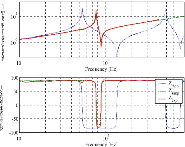
Figure 23 shows the measured point impedance at the middle of the beam. In Figure 24 the same results are shown in a polar plot. Figure 25 shows the coherence of the measurements. The theoretical results in Figure 23 and Figure 24 include the mass of the test rig, but there are still large differences between the two responses. In order to obtain an accurate and suitable model, the parameters of the two dof system were estimated by fitting such a model to the experimental results. The test rig was weighed. The results are reported in Table 12. The mass m1 was increased by 20 grams (about the

weight of the Jelutong and aluminium block) and the mass m2 by 0.5 grams

(approximately the weight of the soldering points). The very good agreement can be see in Figure 23. The stiffness in the model has not been changed.

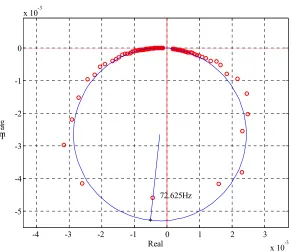
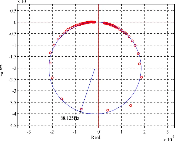
After preliminary checks on the experimental results the circle fitting method was applied to estimate the modal properties of the first mode of the system. Table 13 shows the results of the analysis. Figure 26 and Figure 27 show the results.

(44)

were better without the tape (see Figure 29) because of the not-negligible stiffness of the wires.

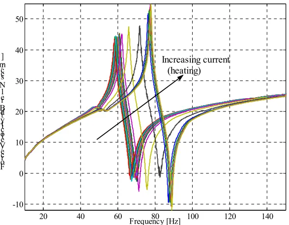
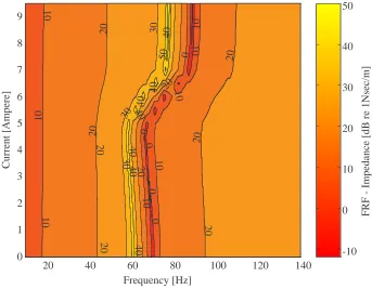
Thermal tests were carried out to find an estimate for the convective coefficient. A current was imposed (see Table 14) and the ambient temperature and that of the wire at the starting and final time of each test were measured. Each test took 5 minutes and six tests were carried out in order to obtain an averaged value. The tests were carried out without vibrating the TVA. For each test, the convective coefficient α has been calculated using the equations 28 and 29. The results, shown in Table 15, show that the average convective coefficient α is 20.53 N/m2K, which is a reasonable value, in accordance with values in the literature.

4.4. SMA test-rig

The SMA TVA was designed in the same way as the brass TVA as described in the subsection 4.2. The mechanical properties used were those given in section 3 (see Table 2 and Table 4). Figure 30 shows the final drawing of the TVA whereas Figure 31 shows the TVA fixed to the impedance head and connected to the shaker.

The theoretical input impedance of the SMA TVA based on a 2dof model is shown in Figure 32, where also the impedance of a steel TVA of the same dimensions is shown. The dimensions of the TVA are shown in Table 16. For the steel a density of 7800 kg/m3 and a Young modulus of 210 109 Pa has been used. For the SMA, a density of 6500 kg/m3 was adopted. The Young modulus of the SMA was set at 40 109 Pa for the cold state (martensitic phase) and 100 109 Pa for the hot state (austenitic phase). As was done for the brass TVA the parameters of an equivalent two dof system were estimated for the SMA TVA and are shown in Table 17.

Finally adopting the same corrections for the masses adopted for the brass test-rig, gave the impedances shown in Figure 33.

4.5. Summary

(45)

Figures

Figure 19 Drawing of the brass test rig

Figure 20 Picture of the brass test rig

101 102 103 104

10-1 100 101 102 103

Frequency [Hz] F

or ce/V el ocit y [N s ec/m ]

Continous Static 2dof

(46)

Figure 22 Outline of the test rig set-up

101 102

100 102

Frequency [Hz] A

mpl itu de F or ce/V el ocit y

Z_theo Z_simp Z_exp

101 102

-100 -50 0 50 100

Frequency [Hz] Pha

se a n gl e [d e gr ee]

Z_theo Z_simp Z_exp

Figure 23 Comparison between calculated and experimental FRF impedance: —— measured; · · · · beam model; - - - - 2 dof approximation

ICP Acc. Test rig

LDS Impedance head PCB Shaker V201

Constant-current

signal conditioner HP spectrum analyser Noise generator Amplifier &

(47)

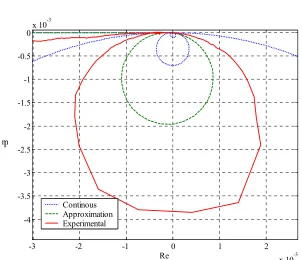
-2.5 -2 -1.5 -1 -0.5 0 0.5 1 1.5 2 2.5 x 10-3 -3.5

-3 -2.5 -2 -1.5 -1 -0.5 0

x 10-3

Re I

m

Continous Approximation Experimental

Figure 24 Polar plot of receptance: —— measured; · · · · beam model; - - - - 2 dof approximation

101 102

0.8 0.85 0.9 0.95 1

Frequency [Hz] Coh

er en ce

(48)

-3 -2 -1 0 1 2 3 x 10-3 -4

-3.5 -3 -2.5 -2 -1.5 -1 -0.5 0 0.5

x 10-3

Real I

ma g

56.5Hz

Figure 26 Circle fitting on the experimental receptance points

0 2

4 6

8 10

0 5

100 0.01 0.02 0.03 0.04 0.05

Frequency lines above resonance Frequency lines

below resonance Los

s fa ct or

(49)

101 102 100

102

Frequency [Hz] F

101 102

0 50 100 150

Frequency [Hz] Pha

se [ de gr ee]

Low Amplitude High Amplitude

Figure 28 Comparison between experimental impedance FRF obtained with different amplitudes of excitation

101 102

100 102

Frequency [Hz] F

101 102

-100 -50 0 50 100

Frequency [Hz] Pha

se [ de gr ee]

With tape Without tape

(50)

Figure 30 Drawing of the SMA test rig

Figure 31 The SMA test rig: the SMA TVA is attached to the shaker through the impedance head

102 100

102

Frequency [Hz] F

102 -50

0 50

Frequency [Hz] Pha

se a n gl e [d e gr ee]

Steel SMA cold SMA hot

(51)

101 102 100

101 102

Frequency [Hz] F

SMA Cold SMA Hot

(52)

Tables

Yield stress Ys 115-390 MPa

Young modulus E 101 GPa Density ρ 8550 kg/m3 Specific heat cp 370 J/(kg K)

Electrical resistivity ρe 62·10-9Ωm

Table 6 Brass (70/30) mechanical properties Total Length L 0.25 m

Diameter d 0.00165 m Table 7 Main dimensions of the brass test rig Modulus of rupture Young modulus Density

YR E ρ

38.6-50.3 GPa 8.0-8.1 GPa 360 kg/m3

Table 8 Jelutong (Dyera costulata) mechanical properties

m1 m2 k fa fr

0.0054 kg 0.0080 kg 1223 N/m ~ 62.2 Hz ~ 97.9 Hz Table 9 Brass vibration neutralizer properties

Accelerometer Sensitivity: -10.2 mV / m·s-2 ±10% and on the signal conditioner x1

Measurement range: ±5V = ±490.5 m·s-2 pk Frequency range (±5%) 1 to 5000 Hz

Force transducer Sensitivity: 22.4 mV / N ±10% and on the signal conditioner x10

A shape memory alloy adaptive tuned vibration absorber: design and implementation

INSTITUTE OF SOUND AND VIBRATION RESEARCH

DYNAMICS GROUP

Design of an adaptive vibration absorbers using shape memory alloy

by

E. Rustighi, M. J. Brennan and B. R. Mace

ISVR Technical Memorandum No. 920

September 2003

Contents

Nomenclature

1. Introduction

2. Tunable vibration absorber (TVA)

2.1. Introduction

2.2. Classical and advanced theory

(

)

(

)

(

)

(

)(

)

(

)(

)

(

)

(

)

(

)

(

)

(

)

(

)

(

)

(

)

(

)

(

)

(

)

(

)

(

)

(

)

(

)

( )

(

(

)

)

( )

(

)

( )

( ) ( )

( )

( )

(

)

( )

( )

[

( )

]

(

)

( )

( )

(

₍

₎

_{( ) ( )}

₍

₎

_{( )}

_∑

_∑

_∑

_∑

₍

₎

_∑

₍

₎