J. Opt. A: Pure Appl. Opt.6(2004) S26–S31 PII: S1464-4258(04)68415-7
Geometric interpretation of the
three-dimensional coherence matrix for
nonparaxial polarization
M R Dennis
H H Wills Physics Laboratory, University of Bristol, Tyndall Avenue, Bristol BS8 1TL, UK
Received 2 September 2003, accepted for publication 30 September 2003 Published 24 February 2004
Online at stacks.iop.org/JOptA/6/S26 (DOI: 10.1088/1464-4258/6/3/005)
Abstract
The three-dimensional coherence matrix is interpreted by emphasizing its invariance with respect to spatial rotations. Under these transformations, it naturally decomposes into a real symmetric positive definite matrix, interpreted as the moment of inertia of the ensemble (and the corresponding ellipsoid), and a real axial vector, corresponding to the mean angular momentum of the ensemble. This vector and tensor are related by several inequalities, and the interpretation is compared to those in which unitary invariants of the coherence matrix are studied.
Keywords: polarization, nonparaxial, density matrix, rotational invariance, irreducible tensor operator
1. Introduction
In the standard theory of partial polarization in paraxial light [1, 2], the 2×2 Hermitian coherence matrix (with unit trace) is decomposed into components with respect to the Pauli matrices. These components, the Stokes parameters, summarize the second order statistical information about the ensemble; in particular, the sum of their squares is unity for a pure polarization state, and zero for a completely unpolarized ensemble.
There has recently been a revival of interest in the corresponding coherence matrix in nonparaxial light, where in general there is no well defined propagation direction, and the Hermitian coherence matrix is 3×3 [3–9]. In these treatments, by analogy with the two-dimensional case, generalized Stokes parameters are defined by decomposing the coherence matrix with respect to the Gell–Mann matrices; a generalized degree of polarization [3–5, 8, 9] may be defined using the sum of squares of these components.
Here, I propose a complementary interpretation of the 3×3 coherence matrix, motivated by geometric reasoning. Rotational, rather than unitary, invariants of the coherence are emphasized, and the matrix is found to decompose into its real part, which is symmetric and interpreted geometrically as an ellipsoid, and its imaginary part, which is antisymmetric and equivalent to an axial vector. The ellipsoid and vector have natural interpretation in terms of the ensemble of polarization states, and are related by certain inequalities to be described.
Pure states are represented by a complex vector E, representing the electric field, in either two or three dimensions. This is represented geometrically by an ellipse by taking Re{Eexp(−iχ)}and varyingχ (this may represent time evolution) [6, 10, 11]; the ellipse therefore has a sense of rotation. In two dimensions, this is taken in the natural sense with respect to the plane, and polarization is either right or left handed. In three dimensions, the plane of the ellipse may vary, and the sense of rotation is a direction normal to the ellipse, defined in a right-handed sense with respect to the ellipse rotation [10, 13]. The eccentricity of the ellipse can be unity (corresponding to linear polarization), zero (corresponding to circular polarization), or any value in between. The ellipses are normalized in units of intensity|E|2. Polarization ensembles
may be visualized geometrically as the set of polarization ellipses in the ensemble, adding incoherently.
The paper proceeds as follows: the following section is a review of conventional two-dimensional coherence matrix theory; in section 3, the geometric decomposition of the 3×3 coherence matrix is described; section 4 is devoted to the properties of the coherence matrix, and section 5 to examples for certain ensembles. The paper concludes with a discussion in section 6.
density matrices (i.e. positive definite matrices with unit trace) will be employed without proof.
2. The two-dimensional coherence matrix
This section is included as a comparison for the 3×3 case, and reviews standard material discussed, for example, in [1, 2, 6]. The two-dimensional coherence matrixρ2, assumed to be
normalized (i.e. trρ2=1), is defined ρ2=
ExEx∗ ExE∗y EyEx∗ EyE∗y
, (2.1) where • denotes ensemble averaging over the ensemble of two-dimensional complex vectors E = (Ex,Ey). ρ2 is
normally expressed in terms of theStokes parameters S1,S2,
andS3, which are the components ofρ2with respect to the Pauli
matrices:
ρ2= 12
1 +S1 S2−iS3 S2+ iS3 1−S1
. (2.2) The three Stokes parameters may be written as a three-vector, theStokes vector
P =(S1,S2,S3) (2.3)
whose length|P|is writtenP.
Being a density matrix, ρ2 is positive definite (its
eigenvalues are non-negative), so
detρ2=(1−S21−S22−S32)/40, (2.4)
that is,
P1, (2.5) which geometrically restrictsP to lie within a sphere of unit radius, thePoincar´e sphere. This fundamental inequality is more commonly derived using the equivalent fact trρ2
2 (trρ2)2.
If the ensemble represents a single state of polarization (i.e. a ‘pure state’), the coherence matrix is idempotent,
ρ2
2,pure=ρ2,pure. (2.6)
Taking the trace implies thatPpure=1. On the other hand, if
the ensemble is completely unpolarized, soρ2,unis 1/2 times
the identity matrix, then Pun=0. This leads to the important
decomposition ofρ2into pure and unpolarized parts, ρ2=(1−P)ρ2,un+Pρ2,pure. (2.7)
The state of polarization corresponding to ρ2,purehere is the
eigenvector corresponding to the larger eigenvalue ofρ2, and
1−Pis twice the smaller eigenvalue.
The previous statements justify P as the degree of polarization. It is invariant with respect to any unitary transformationuρ2u†, by (2.4) (here,urepresents an arbitrary
2×2 unitary matrix). By the well known relation between 2×2 unitary and 3×3 orthogonal matrices, such unitary transformations correspond to rotations of the Stokes vectorP. The operation of a unitary transformation on polarization states (or their ensemble average) is physically interpreted as the operation of a phase retarder [6], and the degree of polarization is unchanged when the ensemble is passed through a retarder, or series of them.
The Stokes vector (2.3) resides in an abstract, three-dimensional (Stokes) space, and the representation of phase retarders by three-dimensional rotations is correspondingly abstract. Ifρ2is transformed by two-dimensional rotations,
corresponding to a real rotation of the transverse plane (i.e.oρ2oT, witho2×2 orthogonal),S
1and S2may change
keepingS2
1+S22constant;S3remains unchanged. An example
case is the rotation in which Reρ2is diagonalized: ρ2,rot= 12
1 +
S12+S22 −iS3
iS3 1−
S2 1+S22
. (2.8)
For pure states, for which the Poincar´e sphere representation is useful, the Stokes parameters provide geometric information about the polarization ellipse [6, 11].
S1and S2inform about the alignment of the ellipse axes, the
major axis making an angle arg(S1+ iS2)/2 with thex-axis. S3
gives the ellipse areaπS3, signed according to polarization
handedness, so S3 is zero for linear, and ±1 for circular
polarization. Obviously, two-dimensional rotations only affect
S1 and S2; the rotation giving (2.8) represents aligning the
major ellipse axis alongx, the minor alongy.
3. Geometry of the three-dimensional coherence matrix
The three-dimensional coherence matrixρ=ρ3is analogous
to (2.1), but withE=(Ex,Ey,Ez):
ρ=
E
xE∗x ExE∗y ExE∗z EyE∗x EyE∗y EyE∗z EzEx∗ EzE∗y EzEz∗
. (3.1)
As before, it is assumed that trρ=1.
The Gell–Mann matrices [15] are the generators of three-dimensional unitary matrices, just as the Pauli matrices generate two-dimensional unitary matrices. Therefore, the
generalized Stokes parametersi,i =1, . . . ,8 [4, 6–9] may
be defined
ρ=1 3
×
1 + 3+8/
√
3 1−i2 4−i5 1+ i2 1−3+8/
√
3 6−i7 4+ i5 6+ i7 1−28/
√
3
.
(3.2) (Other accounts, such as [3], use a different set of generators.) The analogies between (2.2) and (3.2) are obvious: 3 and 8, only appearing on the diagonal, generalizeS1; the terms
in the symmetric, off-diagonal part,1, 4, and7, generalize S2, and 2, 5, and 7, appearing in the antisymmetric,
imaginary part, S3. In particular, if 4, . . . , 7 = 0 and 8 =
√
3/2, then the remaining parameters are proportional to the usual Stokes parameters. This motivates the definition of thegeneralized degree of polarization P3[4, 8, 9] as
P3= 8
i=1 2
i/3. (3.3)
just as in the two-dimensional case, it is invariant with respect to 3×3 unitary transformations. Since(trρ)2−trρ20, it
is readily shown that 0P31.
Although this approach is mathematically correct, it is not clear physically what P3 represents. Unlike the 2×2
case, in which the Stokes vector represents the complete state of polarization using three dimensions (which is easily visualized), the generalized Stokes vector requires eight dimensions, which is not so intuitive.
There is a more serious problem with treating the 3×3 coherence matrix completely in analogy with the 2×2 case— there is no obvious physical interpretation via optical elements of 3 × 3 unitary transformations (nor any corresponding nonparaxial Jones or Mueller calculus). In two dimensions, as an ensemble of plane waves with the same direction but different polarizations propagates through an optical element, the corresponding coherence matrix is transformed by the appropriate Jones matrix, which is unitary for a retarder. In three dimensions, the ensemble of plane waves averaging to the 3×3 coherence matrix does not share a common propagation direction in general; any physical device, represented by a 3 × 3 unitary transformation, should be insensitive to the propagation directions of the separate members of the ensemble. Mathematically, it is possible to find a unitary transformation which takes any three-dimensional state of polarization E = (Ex,Ey,Ez) to any other (leaving |E|2
constant); there is no obvious physical situation in which different states of polarization in three dimensions undergo the same unitary transformation.
It is physically and geometrically natural, however, to consider ρ3 under orthogonal transformations rather than
unitary ones; if viewed as passive rotations, this is simply equivalent to redefining Cartesian axes in three-dimensional space, and no physical operation at all. Clearly, under rotation, where ρ becomes oρoT (o 3×3 orthogonal), the real and
imaginary parts ofρtransform independently of each other. The real part is a positive definite symmetric matrix with five parameters1, 3, 4, 6, and8. Since the (unit) trace is
also unaffected by rotation, it may be considered as distinct from the rest of the real part. The imaginary part is a real antisymmetric matrix with three parameters2, 5, and7,
and in fact the triple(7,−5, 2)transforms under rotation
like an axial vector (noted in [7]). ρtherefore decomposes into three parts: a real scalar (the trace), a real axial vector, and a real traceless symmetric matrix. These different parts (scalar, vector, tensor) are calledirreducible tensor operatorsin group theory; the same decomposition occurs for density matrices of atoms with quantum spin 1, for which the vector part is called theorientationand the tensor part thealignment[16].
From an analytical viewpoint, it is convenient to represent
ρusing Cartesian axesx1,x2, andx3with respect to which the
tensor part is diagonal, giving
ρ=
M
1 −iN3 iN2
iN3 M2 −iN1
−iN2 iN1 M3
. (3.4)
The diagonal elements of (3.4) are restricted:
M1+M2+M3=1, 1M1M2M30, (3.5)
which follows from the fact that the tensor M ≡ Reρ is positive definite. It is geometrically convenient not to separate the scalar and (traceless) tensor parts ofρ, and this is not done in (3.4). Equation (3.4) is analogous to (2.8); the real part
Mhas been (passively) diagonalized, leaving an off-diagonal imaginary part, which transforms as an axial vector
N=(N1,N2,N3) (3.6)
(|N|is invariant under rotations). Mand N have a simple geometrical interpretation, as follows.
The real symmetric matrixMmay be interpreted as the moment of inertia tensor of the ensemble. Geometrically, it is the moment of inertia of the set of polarization ellipses in the ensemble (taking each as an elliptical ring with uniform mass per unit length, insensitive to the ellipse handedness). As with moment of inertia tensors in mechanics, it may be represented in terms of itsinertia ellipsoid, whose points(x1,x2,x3)satisfy
x2 1 M1
+ x
2 2 M2
+ x
2 3 M3
=1. (3.7) The ellipsoid axes are aligned in the 1, 2, and 3 directions, with lengths√M1,
√
M2, and
√
M3. IfM3=0, the ellipsoid is flat (x3 =0). In general, the inertia ellipsoid is specified by six
parameters (the trace and1, 3, 4, 6, 8); the diagonal
form in (3.4), with three parameters, reflects that three Euler angles have been used implicitly in the choice of axes 1, 2, and 3. The traceless part, dependent on theparameters only, gives a measure of departure of this inertia tensor from isotropy. The vector N also has a simple interpretation as half the expectation value for (spin) angular momentum in the ensemble,
¯
S=tr(Sρ)=2N, (3.8) where the spin matricesSi for spin 1 in a Cartesian basis are
given component-wise by Si,j k = −iεi j k [17, 13], withεi j k
the antisymmetric symbol. The axial vectorNis therefore an average of the angular momentum, that is, the average sense of rotation of the ellipses, in the ensemble. Its direction, in general, has no relation to the principal axes ofM(although its maximum length is limited by them, as described in the next section).
The inertia tensorMand orientation vectorN therefore provide information about the real, three-dimensional geometry of the polarization ensemble, and they rotate rigidly. Under more general unitary transformations (which have no physical interpretation), the eigenvalues ofMand components ofN may change arbitrarily (although keeping the unitary invariants trρ,trρ2and detρfixed).
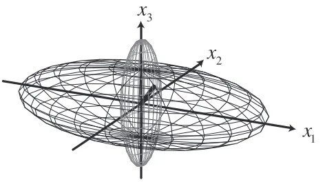
As an example of the geometric interpretation, figure 1 is a representation of the inertia ellipsoid, orientation vector and dual ellipsoid (defined in the next section) for the matrix
ρex= 201
14 −2i 2i
2i 5 −i
−2i i 1
. (3.9)
ρmay also be represented by its eigenvectors; ifρa, ρb,
and ρc represent the pure, idempotent coherence matrices
corresponding to the eigenvectors ofρwith eigenvaluesλa, λb,
andλc(i.e. the principal idempotents [3, 4]), then
Figure 1.The inertia ellipsoid (black mesh), dual ellipsoid (grey mesh), and orientation vector corresponding toρex, in thex1,x2,x3
frame. Here, the orientation vector lies inside the dual ellipsoid, and not on its surface.
The two-dimensional analogue to (3.10) immediately gives rise to the decomposition (2.7). Since the decomposition in (3.10) is in terms of three density matrices, a decomposition in terms of a single purely polarized part and unpolarized part is, in general, impossible (as previously noted in [4, 9]). The eigenvalues ofρ, being unitary invariants, do not have a simple geometric interpretation in terms of the inertia ellipsoid or orientation vector; however, the set of three eigenvectors rotates rigidly. This eigenvector representation ofρprovides a different geometric representation to that given by the inertia ellipsoid and orientation vector. However, it is not geometrically obvious when a given triple of polarization ellipses in three dimensions represent orthogonal polarization states, and solution of cubic equations is required to find the eigenvectors; moreover, the eigenvectors are not uniquely defined at a degeneracy. By comparison, the inertia tensor and orientation vector may be extracted directly fromρ and are always unambiguously defined.
4. Inequalities satisfied byρ
In this section, various inequalities forMandNwill be found, using the fact thatρis a statistical density matrix.
Firstly, the Cauchy–Schwartz inequality may be applied to the off-diagonal elements ofρin (3.1), giving expressions of the form
|ExE∗y|
2|E
x|2|Ey|2. (4.1)
Using the representation (3.4), these imply
N12M2M3, N22M1M3, N32M1M2.
(4.2) Geometrically, this implies that the orientation vector N is confined to a cuboid with vertices (±√M2M3, ±
√
M1M3,
±√M1M2). Sinceρis a density matrix,(trρ)2−trρ20,
that is
N12+N22+N32M2M3+M1M3+M1M2, (4.3)
which is the sum of the inequalities (4.2), and therefore is less strong, geometrically restricting N to lie within the sphere circumscribing the cuboid defined above. (trρ)2−trρ20,
which is the distance by whichNfails to touch the surface of this sphere, is a unitary invariant. The traces of higher powers
ofρsatisfy other inequalities, such as trρ3 trρ2trρ, but
such inequalities can be shown to be consequences of (4.2). Non-negativity of detρimplies that
M1N12+M2N22+M3N32M1M2M3. (4.4)
IfM3=0, then N12 M2M3
+ N
2 2 M1M3
+ N
2 3 M1M2
1, (4.5) which geometrically means thatN lies within the ellipsoid with axes in the 1, 2, and 3 directions, and lengths
√
M2M3,
√
M1M3, and
√
M1M2. This ellipsoid is therefore
circumscribed by the cuboid (4.2), and (4.5) is a stronger inequality than (4.2). The relationship between this ellipsoid and the inertia ellipsoid (3.7) justifies calling this ellipsoid the
dual ellipsoid. IfM3 = 0, (4.4) implies thatN1 = N2 = 0,
and (4.2) gives|N3|
√
M1M2; if the inertia ellipsoid is flat,
the dual ellipsoid is a line normal to it. If M1 = 1,M2 = M3=0, then the inertia ellipsoid is a line andN=0.
As with (2.4), the fundamental inequality for the 3×3 coherence matrix is non-negativity of the determinant, which is stronger than inequalities constructed using the trace. The geometric interpretation of the unitary invariant detρis the product of the distance by which N fails to touch the dual ellipsoid with the dual ellipsoid volume. This quantity, the trace, and the invariant discussed above are the only unitary invariants ofρ. Unlike the two-dimensional case, the properties ofρ are complicated by the fact that polarization information is contained within both the inertia ellipsoidM
and the orientation vectorN.
5. Examples of 3×3 polarization ensembles
Completely unpolarized waves in three dimensions are a common occurrence, for example black body radiation. In this situation, the 3×3 coherence matrix is the completely unpolarized matrix ρun, equal to one-third times the 3×3
identity matrix (andP3=0).
Coherence matrices for pure states of polarization satisfy
ρ2
pure=ρpure. Using (3.4) and (3.5), this implies that ρpure=
M
1 −iN3 0
iN3 M2 0
0 0 0
(5.1)
with|N3| =
√
M1M2,M1+M2 = 1. This is equivalent to
a pure state in two dimensions, and represents a polarization ellipseE = (√M1,±i
√
M2,0)in 1, 2, 3 coordinates. The
ellipse major axis is in the 1-direction, the minor in the 2-direction, and N is normal to the plane of the ellipse (oriented in a right-handed sense of rotation around the ellipse). If M1 = M2 =1/2 in (5.1), the state is circularly polarized,
and N3 = ±1/2. If M1 = 1,M2 = 0 (implyingN3 = 0),
it is linearly polarized. detρpureis zero, but unlike the 2×2
case this is not a sufficient condition for a pure state in general: trρ2must also be unity. The inertia ellipsoid of (5.1) is flat,
If the state is not pure butM3 =0, thenρsatisfies (5.1)
with M1+M2 =1, but|N3|<
√
M1M2. An example is the
density matrix
ρex1= 13
2 0 0
0 1 0 0 0 0
. (5.2)
The inertia ellipsoid here is flat, andN = 0. It cannot be a pure state sinceρ2
ex1=ρex1. This matrix provides an example
of a 3×3 coherence matrix which cannot be decomposed into the sum of a pure polarization matrix and the completely unpolarized matrix, since there is a zero on the diagonal—
ρex1−αρun, for any positiveα, leaves a matrix which is not
positive definite.
It is easy to visualize ensembles which haveN =0: their average angular momentum is zero. This may be achieved, for instance, by requiring, for every Ein the ensemble, that
E∗has the same statistical weight asE. ρ
ex1is therefore the
coherence matrix for the ensemble consisting of the pair of states (with equal weight)
Eex1= {(
√
2,i,0), (√2,−i,0)} (5.3) (of course, this ensemble is not unique in averaging toρex1).
The ellipses corresponding to the pair (5.3) are identical apart from their senses of rotation, which are opposite.
ρex1 is an example of a coherence matrix withN = 0,
although itsMis not isotropic; that is, the shape of the inertia ellipsoid is not constrained by the direction of the orientation vector. More surprising, perhaps, is that the converse is true—the inertia ellipse may be isotropic yetN takes on the maximum value allowed by (4.2), for example
ρex2=13
1 −i 0
i 1 0 0 0 1
, (5.4)
which is the sum of ρun and a completely antisymmetric
matrix (which is not a density matrix). An ensemble which corresponds toρex2is the pair of states with equal weight
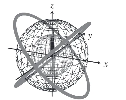
Eex2= {(1,i,−1), (1,i,1)}. (5.5)
The ellipses represented here share their minor axis (in the
y-direction) and have orthogonal major axes. They both have the same shape (eccentricity 1/√2), which geometrically implies that their total moment of inertia is isotropic (higher averages than quadratic are not isotropic). This pair of ellipses, along with the spherical inertia ellipsoid and orientation vector, are shown in figure 2.
Bothρex1 and ρex2 have the same eigenvalues 2/3,1/3,
and 0 (equivalently, the same unitary invariants trρ,trρ2, and
detρ); however, the two ensembles (5.3) and (5.5) are clearly not the same: the ellipses in the two ensembles have the same shape (eccentricity 1/√2), but the orientations in space are different, and there is no obvious physical transformation between the two sets of states.
[image:5.595.320.536.81.252.2]In general, the minimum number of states in an ensemble required to specify ρ is three, and in fact the (complex) eigenvectors of ρ suffice, as in (3.10). In this case, the eigenvectors make up the ensemble, the probability weighting
Figure 2.The pair of polarization ellipses corresponding to the ensemble (5.5) (grey), with their spherical inertia ellipsoid (black mesh), spherical dual ellipsoid (grey mesh), and orientation vector, which here is vertical and on the surface of the dual ellipsoid.
for each being the corresponding eigenvalue. Sinceρex1and ρex2 each have one zero eigenvalue, an ensemble consisting
only of two states is sufficient for these examples (the states in
Eex1andEex2are linear combinations of the eigenvectors, and
are not orthogonal).
6. Discussion
Interfering nonparaxial polarization fields in three dimensions are more complicated than their paraxial counterparts, and their analysis involves subtle geometric reasoning [10, 18, 13, 11]. Most importantly, the Poincar´e sphere description breaks down for polarization states in three dimensions, because it cannot account for the direction of the ellipse normalN; the appropriate nonparaxial analogue of the Poincar´e sphere is the
Majorana sphere, which involves the symmetric product of two unit vectors, which describe the geometry of the nonparaxial polarization ellipse [19, 20, 18]. These two vectors have a complicated expression in terms of the pure field stateE.
It would be of interest to find the relationship between the 3×3 coherence matrix and ensembles defined in terms of the Majorana sphere; a natural physical case would be when theEx,Ey,Ezfield components are Gaussian distributed
(for example black body radiation). In this case, for a given
ρ the distribution on the Majorana sphere would be unique and related to other Gaussian Majorana statistics [21]. The analogous 2×2 distributions on the surface of the Poincar´e sphere have a rather simple form [6, 22–24]. Given the analytical complications of the Majorana sphere, it is unlikely that the 3×3 calculations will be straightforward, and it is unclear whether the geometric interpretation presented here would be helpful in this problem.
such as a Rayleigh particle, responds only to the statistical
Efield at its position, i.e. the coherence matrix. It is therefore possible that classic problems such as atmospheric radiative transfer [25] may be analysed using the 3×3 coherence matrix. A natural experimental situation in which the nonparaxial coherence matrix is relevant is in the optical near field, for which measurements of the three-dimensional field are possible [26] (of course the theory is not restricted to optical frequencies). The geometric interpretation should provide insight into the ensemble of polarization ellipses which gives rise to a measured 3×3 coherence matrix.
Acknowledgments
I am grateful to Michael Berry and John Hannay for useful discussions, and Girish Agarwal for pointing out to me the connection with density matrices in atomic physics. This work was supported by the Leverhulme Trust.
References
[1] Fano U 1949 Remarks on the classical and
quantum-mechanical treatment of partial polarization J. Opt. Soc. Am.39859–63
[2] Mandel L and Wolf E 1995Optical Coherence and Quantum Optics(Cambridge: Cambridge University Press) [3] Samson J C 1973 Descriptions of the polarization states of
vector processes: applications to ULF magnetic fields Geophys. J. R. Astron. Soc.34403–19
[4] Barakat R 1977 Degree of polarization and the principal idempotents of the coherency matrixOpt. Commun.23
147–50
[5] Samson J C and Olson J V 1980 Some comments on the descriptions of the polarization states of wavesGeophys. J. R. Astron. Soc.61115–29
[6] Brosseau C 1998Fundamentals of Polarized Light: a Statistical Optics Approach(New York: Wiley) [7] Carozzi T, Karlsson R and Bergman J 2000 Parameters
characterizing electromagnetic wave polarizationPhys. Rev. E612024–8
[8] Set¨al¨a T, Kaivola M and Friberg A T 2002 Degree of polarization in near fields of thermal sources: effects of surface wavesPhys. Rev. Lett.88123902
[9] Set¨al¨a T, Shevchenko A, Kaivola M and Friberg A T 2002 Degree of polarization for optical near fieldsPhys. Rev.E
66016615
[10] Nye J F 1999Natural Focusing and Fine Structure of Light: Caustics and Wave Dislocations(Bristol: Institute of Physics Publishing)
[11] Dennis M R 2002 Polarization singularities in paraxial vector fields: morphology and statisticsOpt. Commun.213
201–21
[12] Fano U 1957 Description of states in quantum mechanics by density matrix and operator techniquesRev. Mod. Phys.29
74–93
[13] Berry M V and Dennis M R 2001 Polarization singularities in isotropic random vector wavesProc. R. Soc.A457141–55 [14] Sakurai J J 1994Modern Quantum Mechanicsrevised edn
(Reading, MA: Addison-Wesley)
[15] Griffiths D 1987Introduction to Elementary Particles(New York: Wiley)
[16] Blum K 1996Density Matrix Theory and Applications2nd edn (New York: Plenum)
[17] Altmann S L 1986Rotations, Quaternions, and Double Groups(Oxford: Oxford University Press)
[18] Dennis M R 2001 Topological singularities in wave fieldsPhD ThesisBristol University
[19] Penrose R 1989The Emperor’s New Mind(Oxford: Oxford University Press)
[20] Hannay J H 1998 The Majorana representation of polarization, and the Berry phase of lightJ. Mod. Opt.451001–8 [21] Hannay J H 1996 Chaotic analytic zero points: exact statistics
for a random spin stateJ. Phys. A: Math. Gen.29L101–5 [22] Barakat R 1987 Statistics of the Stokes parametersJ. Opt. Soc.
Am.A41256–63
[23] Eliyahu D 1994 Statistics of Stokes variables for correlated Gaussian fieldsPhys. Rev.E502381–4
[24] Brosseau C 1995 Statistics of the normalized Stokes parameters for a Gaussian stochastic plane wave fieldAppl. Opt.344788–93
[25] Chandrasekhar S 1950Radiative Transfer(Oxford: Oxford University Press)