An information theoretic approach for knowledge representation using Petri nets

An information theoretic approach for knowledge

representation using Petri nets

Manuel Chiachío, Juan Chiachío, Darren Prescott and John Andrews

Faculty of Engineering University of Nottingham Nottingham, NG7 2RD, UK

Email:{manuel.chiachio, juan.chiachioruano, darren.prescott, john.andrews}@nottingham.ac.uk

Abstract—A new hybrid approach for Petri nets (PNs) is proposed in this paper by combining the PNs principles with the foundations of information theory for knowledge represen-tation. The resulting PNs have been named Plausible Petri nets (PPNs) mainly because they can handle the evolution of a discrete event system together with uncertain (plausible) information about the system usingstates of information. This paper overviews the main concepts of classical PNs and presents a method to allow uncertain information exchange about a state variable within the system dynamics. The resulting methodology is exemplified using an idealized expert system, which illustrates some of the challenges faced in real-world applications of PPNs.

Keywords—Petri nets; Expert Systems; Knowledge representa-tion

I. INTRODUCTION

A. Classical Petri Nets

Petri Nets (PNs) are bipartite directed graphs (digraph) used for modeling the dynamics of systems, which are known after the celebrated thesis dissertation Kommunikation mit Automaten by Carl Petri in 1962 [1]. Two types of nodes are represented in a PN: transitions and places, which are temporarily visited bytokens, the abstract moving units of a PN that can adopt different meanings depending on the application (also different meanings within a specific PN). The distribution of tokens over the PN at a specific time of execution is referred to as marking.

From a mathematical perspective, a PN can be defined as an ordered 6-tupleP as follows [2]:

P_,hP,T,E,M0,D,Wi (1)

where P ∈ Nnp _{and T ∈}

Nnt _{are vectors to denote the} set of np places and nt transitions of the PN respectively,

M0 ∈ Nnp _{is the initial marking, and D ∈}

Rnt _{is the} non-negative vector of switching delays of the transitions (0 by default). The connections between transitions and places are expressed through the set of edgesE⊆(P×T)∪(T×P), so thatE⊂Nnp_×

Nnt_{contains ordered pairs of nodes. Each edge} (also referred to as arc) has assigned a weight, a non-negative integer value (1 by default) defined in the set of weightsW.

There are three main laws that govern a PN, that can be enunciated as follows:

1) Transitions always consume from all the input arcs at the same time;

2) Transitions always produce from all out-coming arcs the same amount;

3) Transitions cannot consume tokens from an empty place.

The dynamics of classical PNs can be described through a state equation defined as follows:

Mk+1=Mk+ATuk (2)

whereukis thefiring vectorat statek, annt-dimensional

vec-tor of Boolean values whose elements are obtained according to the firing rule, as will be explained further below.Ais an

nt×np matrix typically referred to as the incidence matrix,

whose elements are the result of subtracting the forward (A+_{)andbackward(A}−_{)incidence matricesrespectively, as}

follows:

A=A+−A− (3) where

A+= 

  

a+₁₁ a+₁₂ ··· a+_1np a+₁₂ a+₂₂ ··· a+_2np

..

. . ..

a+_nt1a+_nt2 ··· a+ ntnp



  

A−= 

  

a−₁₁ a−₁₂ ··· a−_1np a−₁₂ a−₂₂ ··· a−_2np

..

. . ..

a−_nt1a−_nt2 ··· a−_ntnp



  

(4)

In the last equation, the element a+ij is the weight of the arc

from transitiontito output placepj, whereasa−ij is the weight

of the arc to transition ti from input place pj, where i =

1, . . . , nt,j= 1, . . . , np. If transitionti is activated at statek,

thenui,k∈uk is modified according to the firing rule, which

can be expressed as follows:

ui,k=

(

1, if M(j)>a−ij ∀pj∈ •Pti

0, otherwise (5)

whereM(j)∈_Nis the marking for placepj, and•Ptidenotes the set of places that belong to the pre-set of transition ti, i=

1, . . . , nt, as will be next described.

B. Tokens, probability, and information

reality of certain systems [3], [4]. From the last years, a signif-icant increase in the research activity has been observed in the literature about the definition of new kind of tokens as a way to make PNs better aligned with the reality of the systems to be idealized. Traditionally, tokens in classical PNs are interpreted as moving objects (typically integer units) in a network of interconnected places, as mentioned in Section I-A. Further approaches encountered in the literature consider different kind of tokens, like for example numerical tokens [5], [6], fuzzy tokens [4], [7], particle tokens [8], [9], to cite just but any, each one providing some changes on the net dynamics, yet defining a variant of the classical PNs.

In this work, a hybrid approach is proposed by combining traditional tokens with a new class of tokens that represent a degree of belief about a state variable at a certain mode which is specified by a place. The resulting framework has been named Plausible Petri Nets (PPN) since certain tokens enclose a set of numerical values about a state variablexfrom a finite-dimensional set X ⊂ _Rd_{, along with a mapping over}

X denoted byf :X ⊂→R+that assigns each elementxwith a non-negative value interpreted as itsrelative plausibility, as will be discussed in the next section. In PPNs, the moving units are objects (in the sense of integer units as in classical PNs) and also states of information about x. Moreover, the consumption and production of tokens in PPNs are not only associated with the concept of adding and subtracting integer values, but also with the operation of adding and subtracting information about the state variable x.

The next section provides further insight into the concepts of plausibility, uncertainty, and states of information, since they are fully adopted throughout the text. Section III is devoted to providing the basis and main rules of the proposed PPNs. In Section IV, our framework is illustrated using an example of application. Finally, Section V gives concluding remarks.

II. BASIC OPERATIONS INPLAUSIBLEPETRI NETS

Let A ⊆ X be a subset representing a certain event or proposition overX in such a way that there exist a probability measure P(A) through a density function f(x) that can be normalized such that R

Xf(x)dx = 1. In this sense, P(A)

is interpreted as the plausibility of a set of possible values

x given a state of information about them provided by f(x)

[10]–[12]. Let us now evoke the first principles of Boolean logic by recalling the concepts of the logic operatorsAND (∧) andOR(∨) for the conjunction and disjunction of propositions, respectively. Then, the following logical relationships are com-patible according to the De Morgan’s law [13], [14] for two probability measures Pa(A)andPb(A), each one ascribed to

the state of information fa(x)andfb(x), respectively:

Pa(A) = 0 OR Pb(A) = 0 ⇒ (Pa∧Pb)(A) = 0

Pa(A)6= 0 OR Pb(A)6= 0 ⇒ (Pa∨Pb)(A)6= 0

(6) where (Pa ∧Pb)(A) and(Pa∨Pb)(A) can be expressed as

[15]:

(Pa∧Pb)(A) =

Z

A

(fa∧fb)(x)dx (7a)

(Pa∨Pb)(A) =

Z

A

(fa∨fb)(x)dx (7b)

In the last equation, the densities(fa∧fb)(x)and(fa∨fb)(x)

represent theconjunctionanddisjunction of states of informa-tion given by fa(x), fb(x), respectively [12], [16]. Besides,

(Pa∧Pb)(A)and(Pa∨Pb)(A) stand for the plausibility of

the set of values x ∈ Ain compliance with the information given by (fa∧fb)(x) and(fa∨fb)(x), respectively.

Next, because commutativity is allowed in logic of proposi-tions, i.e.(Pa∨Pb)(A) = (Pb∨Pa)(A)and (Pa∧Pb)(A) =

(Pb ∧Pa)(A), then a simple solution for the unnormalized

densities (fa∧fb)(x)and(fa∨fb)(x)are such that [17]:

(fa∨fb)(x) =fa(x) +fb(x) (8a)

(fa∧fb)(x) =

fa(x)fb(x)

µ(x) (8b)

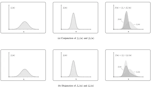
where µ(x) is the homogeneous density function [12], [18], a reference state of information that can be understood as a probability model for x ∈ X in absence of any other information, which actually represents the state of total ig-norance aboutX [18], [19]. In case thatX is a linear space, it is demonstrated [17] that µ(x) = const, i.e., µ(x) is a uniform over X. See Fig. 1 for a conceptual illustration of the conjunction and disjunction of states of information over some arbitrary densitiesfa(x)andfb(x). Moreover, it is worth

noting that the conjunction and disjunction operations over states of information can be extended to the case of multiple states of information(e.g.f1(x), f2(x), . . . , fn(x)), as follows

[18]:

(f1∨ · · · ∨fn)(x) = n

X

i=1

fi(x) (9a)

(f1∧ · · · ∧fn)(x) = n

Y

i=1

fi(x)

µ(x) (9b)

Finally, observe that the normalization of the density function in (8b) may require the evaluation of an intractable integral such that R

X

1

α

fa(x)fb(x)

µ(x) dx = 1, where α is a normaliz-ing constant. Moreover, note that there might be situations where the conjunction is conducted with density functions which are not completely known, perhaps because they are defined trough samples. Hence, sampling-based algorithms (e.g. particle methods) [20], [21] can be used in those cases to circumvent the evaluation of the normalizing constant. In particle methods, a set ofN samples {x(n)_}N

n=1 with associ-ated weights {w(n)_}N

n=1 are used to obtain an approximation for the required density function [e.g. (fa ∧fb)(x)] with a

feasible computational cost, as follows:

(fa∧fb)(x)≈ N

X

n=1

w(n)δ(x−x(n)) (10)

where x(n) _{∼ (f}

a ∧fb)(x), and δ is the Dirac delta. The

particle weight w(n) _{represents a likelihood value of then-th} particle, which can be obtained as follows:

w(n)₌ fa(x(n))fb(x(n))

PN

n=1fa(x(n))fb(x(n))

(11)

fa(x)

x

fb(x)

x

fa(x)

fb(x) f(x) = (fa∧fb) (x)

x

(a) Conjunction offa(x)andfb(x)

fa(x)

x

fb(x)

x

fa(x)

fb(x) f(x) = (fa∨fb) (x)

x

(b) Disjunction offa(x)andfb(x)

Fig. 1. Illustrative example of the conjunction and disjunction operation over two states of information, namelyfa(x)(left panels) andfb(x)(center panels). The

right panels represent the resulting densityf(x)from the conjunction (upper right) and disjunction (lower right) offaandfb. The resulting PDF is represented

superimposed overfaandfbfor better understanding.

III.INFORMATION FLOW DYNAMICS INPPNS

A. Modelling assumptions

Let {xk, k ∈ N} be a stochastic process taking values in

X, which is manifested through different modes corresponding to each place of the Petri net. Next, let us consider thatP∈P can be partitioned into two disjoint sets: 1) numerical places

P(N) _∈

Nnp_{, and 2) symbolic places} P(S) ∈

Nn 0

p_{, such}

that P(N)_{∪ P}(S) _{= P ∈}

Nnp+n 0

p_{, and} P(N) ∩P(S) = ∅. Analogously, the set of transitions T is partitioned into numerical transitions T(N) _∈

Nnt, and symbolic transitions T(S) _∈

Nn 0

t_{, where} T(N) ∪ T(S) = T ∈ _Nnt+n0t_{, and}

T(N)_∩T(S)_{6=∅. Those transitions that belong toT}(N)_∩T(S) are referred to as mixed transitions. Finally, let us call by

•_Pt

i, the subset of places from the pre-set of transition

ti, i= 1, . . . , nt. AnalogouslyP•ti is to denote the subset of places that belongs to the post-set of ti. From this standpoint,

the dynamics of PPNs is formulated under the adoption of the following items:

1) At a certain time k, the place p(_jN) encloses a state of information about xk given by f

pj

k , where f pj

k : Aj →

R+ andAj is a subset ofX;

2) Equivalently, any transition ti ∈ T(N) carries a state

of information about xk defined over Ai ⊆ X, namely

fti k(xk);

3) As in classical PNs, there exist arc weights for the symbolic places, denoted by a0ij+, a

0

−

ij ∈ W(S) ⊂ N,

whereby the incidence matrix A(S) _{can be obtained as:}

A(S) _=a0+

ij −a

0

−

ij , i= 1, . . . , n0t, j = 1, . . . , n0p, where

n0

p,n0tare the number of symbolic places and transitions

of the PPNs, respectively. The arc weights for the numer-ical places are denoted bya+ij, a−ij ∈W(N)⊂R+, where

A(N) _{= a}+

ij −a−ij, and i = 1, . . . , nt, j = 1, . . . , np,

being in this casent,np the amount of numerical

transi-tions and numerical places of the PPN, respectively. These weights provide us with a measure of the importance of the information that flows from/to the corresponding transition;

4) Any transitionti always consumes from all its input arcs

at the same time. Moreover, an input arc from placep(jN)

to transition ti ∈ T(N) conveys a state of information

given by the conjunction of states of information of

fpj

k (xk)andfkti(xk), namely(f pj

k ∧f

ti k )(xk);

5) Any transition ti produces to its output arcs the same

amount of information given by the conjunction of states of information between fti

k(xk) and f

•_P

ti_{(xk), i.e.,}

(fti

k ∧ f

•_P

ti_{)(xk). In the last expression, f}•Pti_(xk) results from the disjunction of the states of information of the pre-set of transitionti, i.e.,f

•_P

fp_ti,2 _{∨ · · · ∨ f}pti,m_{)(xk) (recall [9a]), where places}

pti,1, pti,2, . . . , pti,m∈ •Pti⊂P (N)_;

6) If numerical placep(jN) belongs to the pre-set ofti, and

assuming that1 _p(N)

j ∈/ P•t˜_i ∀˜i= 1, . . . , nt, then the state

of information that remains inp(_jN) atk+ 1after firing

ti, is the conjunction of f pj

k (xk) and fkti(xk) weighted

according toa−ij, i.e.f pj

k+1(xk+1) =a−ij(f pj k ∧f

ti k)(xk);

7) Correspondingly, the state of information resulting in place p(_˜jN) after firing ti given that p(jN) ∈ P•ti, is the disjunction of the states of information fpj

k (xk)and

(fti

k ∧f

•_P

ti_{)(xk), where the latter is multiplied by its}

output weighta+_ij. Mathematicallyfpj

k+1(xk+1) =

fpj

k ∨

a+_ijfti k ∧f

•_P

ti _(xk).

Observe that the rules given above, specifically those from items 3) and 5), are in agreement with the rules of classical PNs given in Section I-A except for the consideration that here, part of the flow of tokens is based on states of information.

B. Marking evolution

In PPNs, the marking at state k consists of both types of information given by M(kN) for the numerical

places, and M(kS) for the case of symbolic places, so

that Mk =

M(kN),M

(S)

k

. Mathematically, M(kN) is

ex-pressed through a column vector specified by M(kN) =

f_kp1(xk), f_kp2(xk), . . . , f p_np k (xk)

T

, such that each fpj k (xk)

is a normalized density function that provides us with a measure of the relative plausibility of xk at place p

(N)

j ,

j = 1, . . . , np. Similarly,M

(S)

k is expressed through a column

vector of integer values so that itsjth component represents the number of tokens present in placep(jS)at statek. The marking

evolution ofM(kS) for the symbolic subnet has been given in

(2), which corresponds to the state equation of an ordinary PN [2]. However, the marking evolution corresponding to the numerical places gives response to the information flow dynamics described in Section III-A, and in particular, results from applying the rules 4) to 7). Both markings, namelyM(_kN)

and M(_kS), evolve in a synchronized manner driven by the firing rule for PPNs, as will be explained below.

C. Firing rule for PPNs

In PPNs, any transition ti ∈ T is fired at state k if the

delay time has passed and:

1) ∀p(jS) ∈ •Pti, M (S)

k (j) > a

0

−

ij, for ti ∈ T(S), ti ∈/

(T(S)_∩T(N)_);

1_{The assumption implies that placep}(N)

j does not belong to the post-set

of any transition.

2) ∀p(jN)∈ •Pti, (f pj k ∧f

ti

k )(xk)6=∅, which, in this case,

applies for numerical transitions, i.e., ti ∈ T(N), ti ∈/

(T(S)_∩T(N)_);

3) Condition 1) and 2) are both satisfied for numerical places and symbolic places from the pre-set of ti, whenti is a

mixed transition, i.e. ti∈(T(S)∩T(N)).

Condition 1) means that each symbolic place from the pre-set of ti has enough amount of tokens according to their input

arc weight, as in classical PNs. On the other hand, condition 2) allows us to ensure that every conjunction of states of information between fti _{and each of the density functions} from the pre-set of ti, are possible. Note that a conjunction

(e.g. (fpj

k ∧f

ti

k )(xk)) is possible if (f pj

k ∧f

ti

k)(xk) 6=∅ for

any subset B ∈ X [12].

IV. APPLICATION EXAMPLE

In this section, a numerical example is provided to illustrate our proposed methodology. To this end, let us consider that there exist a measurement about a bi-dimensional state variable

xk= (x1,k, x2,k), performed using two sensors denoted bys1 ands2. The information froms1ands2is initially represented in placesp(1N)andp

(N)

2 using probability densities as respec-tive states of information aboutxk. Suppose now that the

sen-sors are imperfect so that they introduce uncertainty that can modeled as a zero mean Gaussian density function with covari-ance matrix given by Σ1 andΣ2, respectively. Next, consider that the component-wise measurements are stochastically inde-pendent so that Σ1 =diag(σv21, σ

2

v2), Σ2 =diag(σ

2

w1, σ

2

w2),

where σv1, σv2, σw1, σw2 are the standard deviations of

mea-surement errors v = (v1, v2) andw = (w1, w2), for sensors

s1 and s2, respectively. The system being modeled is based on an expert system that controls the activation of a discrete-event subsystem (which can represent an automata, machine, or similar, in a real-world application). Once a new data point arrives, then the activation/deactivation of the discrete subsystem occurs conditioned upon the quality of the infor-mation coming from the sensors. The differential entropy, as a measure of the data uncertainty, is used in this example as a quality indicator of the information given by the sensors. Fig. 2 provides a geometric description of the PPN being modeled using four numerical places (p(1N) to p

(N)

4 ), five symbolics places (p(₁S) to p(₅S)), and three mixed transitions labeled as

t1, t2, and t3. A cold transition () is used to represent the data arrival to the system. In our PPN model, the information from sensors s1 and s2, initially represented in places p(1N) and p(2N), is further gathered in place p

(N)

3 provided that transition t1 is fired. The joint information in place p(3N) is then used to activate a sequence of discrete-event system (e.g. a machine) if the differential entropy of xk is lower than a

certain reference value ξ ∈ R, which is taken as ξ = 7 in this example. Next, the state of information aboutxk is finally

collected in place p(4N). Otherwise, transition t2 is activated whereby the information in place p(₂N) is improved using the joint information aboutxk given in placep(3N). Note thatp

The initial marking for the numerical places is

M(0N) =

f0p1(x0), f0p2(x0), f0p3(x0), f0p4(x0)

T

, where

fp1

0 ∼ N(ˆx,Σ1), f0p2 ∼ N(ˆx+β,Σ2),f0p3 =f

p4

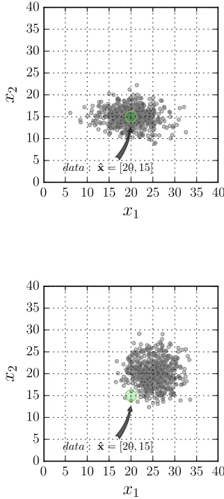
0 =∅. In the last expressions, ˆx is the data point that arrives to the system, and βis a bias that applies to the measurements from sensor s2. In this example, xˆ = (20,15), and β = (5,5), both expressed in arbitrary units. The covariance matrices for f0p1(x0) and f0p2(x0) are given by Σ1 = diag(42,32) and Σ2 = diag(32,32), respectively. See Fig. 3 for a particle-based representation of the states of information for places p(1N)andp

(N)

2 atk= 0.

On the other side, the initial marking for symbolic places is given by M(0S)= (0,0,0,0,1)

T

. The mixed transitionsti,

i={1,2,3}are defined using Diract Delta density functions, i.e., fti(x

k)∼IBi(xk), thus their firing is prescribed for the state variable xk on fulfilling the conditionxk∈ Bi, where:

B1=nxk∈ X : (x1,k−20)2+ (x2,k−20)2610

o

(12a)

B2=nxk∈ X :H(xk)>ξ

o

(12b)

B3=nxk∈ X :H(xk)< ξ

o

(12c)

In (12b) and (12c), H : X → R denotes the differen-tial entropy of xk, that can be obtained by calculating2

1_/2ln

(2πe)d_{det [cov(x} k)]

as a measure quantifying the un-certainty of xk. Here, we assume for simplicity that the time

spent by the machine in performing transitions t4 and t5 is negligible. The rules for the information flow dynamics of PPNs [recall rules 4) to 7) in Section III-A] along with (2), are applied in confluence with the firing rule for the system state evolution described through the markingMk. The

particle approximation for conjunction of states of information described in Section II, has been applied to evaluate the conjunction of states of information resulting from applying

2_{This expression for the differential entropy is actually an upper-bound}

approximation to the actual differential entropy, where the exactness is achieved when the density function is Gaussian.

p(S)1

p(N)1

p(N)2

p(N)3

p(S)2 2 t1

p(5S)

p(N)4 p(S)3 p(4S)

2

t2 t3

t4 t5

Fig. 2. Plausible Petri net of example in Section IV. Numerical places and transitions are represented using double line to distinguish them from the symbolic ones. Transitionst4,t5, and placep(S)4 under the dashed box

represent a discrete-event subsystem in a simplified manner.

0 5 10 15 20 25 30 35 40

x

0 5 10 15 20 25 30 35 40

x

data: xˆ= [20,15]

0 5 10 15 20 25 30 35 40

x

0 5 10 15 20 25 30 35 40

x

data: xˆ= [20,15]

Fig. 3. Representation of the density functionsfp1

k (xk)andfkp1(xk)for

k= 0using samples (circles) in thex-space. The green circle represents a data point arrived to the system.

rules 4) to 7) from the information flow dynamics for the numerical subnet. The disjunction of states of information are straightforwardly evaluated using samples by just joining the samples from the component-wise density functions, and af-fecting their particle weights using an appropriate normalizing constant so as to obtain a bone fide density.

The results for the numerical places are presented for states

k = 0 and k = 2 in Fig. 4 (the states of information about

xk remain unchanged in P(N) after k = 2, hence they are

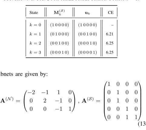
not represented). A summary of the results for the analysis of the PPN is provided in Table I. Note from Table I that the results for symbolic marking and active transitions are column vectors, although they are not explicitly reflected as so in this table for clarity. Also, the fourth column represents the continuum entropy offp3

k (xk), k = 1,2,3. The incidence

TABLE I. SUMMARY OF THE RESULTS FROM THE ANALYSIS OF THE

PPNSHOWN INFIG. 2FOR THREE STATES STARTING FROMk= 0.

State M(_kS) uk CE

k= 0 (1 0 0 0 0) (1 0 0 0 0) –

k= 1 (0 1 0 0 0) (0 0 1 0 0) 6.21

k= 2 (0 0 1 0 0) (0 0 0 1 0) 6.25

k= 3 (0 0 0 1 0) (0 0 0 0 1) 6.25

subnets are given by:

A(N)₌





−2 −1 1 0

0 2 −1 0 0 0 −1 1



,A(S)= 

     

1 0 0 0 0 1 0 0 0 1 0 0 0 0 1 0 0 0 1 1



     

(13)

respectively. Observe from the analysis that numerical and symbolic subnets interact theirselves in a synchronized man-ner. To serve as an example, note that transitiont1is activated after the data arrival at k = 0 because p(₁S) is assigned one token and (fpi

0 ∧f

t1

0 )(xk) 6=∅, for i = 1,2. Note also that

t1 is no longer fired at k >1 because p(1S) is empty, hence condition 1) from the firing rule is not fulfilled. The sequence of discrete-event actions (marked using a dashed box in Fig. 2) are activated at k = 2 after t3 is fired, since the entropy condition given through t3 is fulfilled at such time. Note that this example demonstrates that the flow of information can be altered (activate/deactivate) in our PPNs by combining numerical and symbolic places so as to make their tokens conveniently interact in a synchronized manner. The results for the numerical places p(1N) and p

(N)

4 are presented for states

k= 0tok= 2in Fig 4.

V. CONCLUSION

A novel hybrid approach for PNs has been proposed in this paper by combining the algebra of classical PNs with the basis of information theory. As in classical PNs, there exist a set of places and transitions (labeled here as "symbolic") to model discrete-event systems using regular tokens as moving units. In addition, a set of numerical places and transitions are considered to model knowledge representation about a system state variable, which interact with the regular tokens in a synchronized manner. The simulated results demonstrate that PPNs are a versatile tool to fuse uncertain information (which can be diverse through the different numerical nodes) about the state variable with sequences of Boolean events, provided that an adequate net architecture is adopted. This fact makes them useful for analyzing hybrid systems with interaction of diverse sources of information, like in expert systems. One future research direction is to explore their ability to model cybersystems, since they can receive, store, exchange, and process information so as to use it for control. Moreover, further research effort is needed to investigate formal aspects of the resulting hybrid system, as well as to explore efficient implementations using a variety of examples of application.

ACKNOWLEDGMENT

5 10 15 20 25 30 35

x1 5

10 15 20 25 30 35

x2

5 10 15 20 25 30 35

x1 5

10 15 20 25 30 35

x2

5 10 15 20 25 30 35

x1 5

10 15 20 25 30 35

x2

5 10 15 20 25 30 35

x1 5

10 15 20 25 30 35

x2

(a) States of information aboutx0

5 10 15 20 25 30 35

x1 5

10 15 20 25 30 35

x2

5 10 15 20 25 30 35

x1 5

10 15 20 25 30 35

x2

5 10 15 20 25 30 35

x1 5

10 15 20 25 30 35

x2

5 10 15 20 25 30 35

x1 5

10 15 20 25 30 35

x2

(b) States of information aboutx1

5 10 15 20 25 30 35

x1 5

10 15 20 25 30 35

x2

5 10 15 20 25 30 35

x1 5

10 15 20 25 30 35

x2

5 10 15 20 25 30 35

x1 5

10 15 20 25 30 35

x2

5 10 15 20 25 30 35

x1 5

10 15 20 25 30 35

x2

(c) States of information aboutx2

Fig. 4. PPN output for numerical placesp(N)₁ (most-left panel) top(N₄ )(most-right panel). Each subplot represents the state of information aboutxk, using samples (circles) in the state spaceX.

REFERENCES

[1] C. A. Petri, “Kommunikation mit automaten,” Ph.D. dissertation, Institut für Instrumentelle Mathematik an der Universität Bonn, 1962. [2] T. Murata, “Petri nets: Properties, analysis and applications,”

Proceed-ings of the IEEE, vol. 77, no. 4, pp. 541–580, 1989.

[3] J. Cardoso, R. Valette, and D. Dubois, “Possibilistic Petri nets,”IEEE Transactions on Systems, Man, and Cybernetics, Part B: Cybernetics, vol. 29, no. 5, pp. 573–582, 1999.

[4] Z. Ding, Y. Zhou, and M. Zhou, “Modeling self-adaptive software systems with learning Petri nets,” in Companion Proceedings of the 36th International Conference on Software Engineering. ACM, 2014, pp. 464–467.

[5] G. Horton, V. G. Kulkarni, D. M. Nicol, and K. S. Trivedi, “Fluid stochastic Petri nets: Theory, applications, and solution techniques,”

European Journal of Operational Research, vol. 105, no. 1, pp. 184– 201, 1998.

[6] M. Silva, J. Júlvez, C. Mahulea, and C. R. Vázquez, “On fluidization of discrete event models: observation and control of continuous Petri

nets,”Discrete Event Dynamic Systems, vol. 21, no. 4, pp. 427–497, 2011.

[7] S.-M. Chen, J.-S. Ke, and J.-F. Chang, “Knowledge representation using fuzzy Petri nets,”Knowledge and Data Engineering, IEEE Transactions on, vol. 2, no. 3, pp. 311–319, 1990.

[8] C. Lesire and C. Tessier, “Particle Petri nets for aircraft procedure monitoring under uncertainty,” inApplications and Theory of Petri Nets 2005: 26th International Conference, ICATPN 2005, Miami, USA, June 20-25, 2005. Proceedings, G. Ciardo, Ed. Springer, 2005, pp. 329–348. [9] L. Zouaghi, A. Alexopoulos, A. Wagner, and E. Badreddin, “Modified particle Petri nets for hybrid dynamical systems monitoring under envi-ronmental uncertainties,” inSystem Integration (SII), 2011 IEEE/SICE International Symposium on. IEEE, 2011, pp. 497–502.

[10] R. T. Cox, “Probability, frequency and reasonable expectation,” Amer-ican journal of physics, vol. 14, p. 1, 1946.

[11] E. Jaynes,Papers on probability, statistics and statistical physics. (Ed. R.D Rosenkrantz), Kluwer Academic Publishers, 1983.

Journal of Geophysics, vol. 50, no. 3, pp. 159–170, 1982. [13] I. M. Copi,Introduction to logic. New York, Macmillan, 1953. [14] R. L. Goodstein,Boolean algebra. Dover Publications, Inc., 2007. [15] A. Kolmogorov,Foundations of the Theory of Probability (Translation

of 1933 original in German). Chelsea Publishing: New York, 1950. [16] G. Rus, J. Chiachío, and M. Chiachío, “Logical inference for inverse

problems,”Inverse Problems in Science and Engineering, vol. 24, no. 3, pp. 448–464, 2016.

[17] A. Tarantola,Inverse problem theory and methods for model parameters estimation. SIAM, 2005.

[18] K. Mosegaard and A. Tarantola, “Probabilistic approach to inverse problems,” inInternational Handbook of Earthquake and Engineering Seismology, Part A, ser. International Geophysics. Academics Press Ltd, 2002, vol. 81, pp. 237–265.

[19] E. T. Jaynes, “Prior probabilities,” Systems Science and Cybernetics, IEEE Transactions on, vol. 4, no. 3, pp. 227–241, 1968.

[20] M. Arumlampalam, S. Maskell, N. Gordon, and T. Clapp, “A tutorial on particle filters for on-line nonlinear/non-Gaussian Bayesian tracking,”

IEEE Transactions on Signal Processing, vol. 50, no. 2, pp. 174–188, 2002.