City, University of London Institutional Repository
Citation
:
Yearsley, J. (2017). Advanced tools and concepts for quantum cognition: A
tutorial. Journal of Mathematical Psychology, 78, pp. 24-39. doi: 10.1016/j.jmp.2016.07.005
This is the accepted version of the paper.
This version of the publication may differ from the final published
version.
Permanent repository link:
http://openaccess.city.ac.uk/18713/
Link to published version
:
http://dx.doi.org/10.1016/j.jmp.2016.07.005
Copyright and reuse:
City Research Online aims to make research
outputs of City, University of London available to a wider audience.
Copyright and Moral Rights remain with the author(s) and/or copyright
holders. URLs from City Research Online may be freely distributed and
linked to.
City Research Online: http://openaccess.city.ac.uk/ [email protected]
Advanced tools and concepts for quantum cognition: A tutorial
IJames M. Yearsleya,b
aDepartment of Psychology, School of Arts and Social Sciences, City University London, Whiskin Street, London EC1R 0JD, UK bJDM Lab, Department of Psychology, Vanderbilt University, Nashville, TN 37240-7817, USA
Abstract
This tutorial is intended to provide an introduction to some advanced tools and concepts needed to construct more realistic quantum models of decision. The aim is to cover, in a format suitable for researchers with some limited exposure to quantum models of cognition, the ideas of density matrices, POVM type measurements and open system dynamics. The central theme we explore is how we might introduce noise into our quantum models, and the effect this has on model behaviour. These important ideas are likely to be very useful for constructing more realistic cognitive models, but they are generally not covered by introductory accounts of quantum theory. We hope that this tutorial will help to introduce these tools to other researchers interested in constructing quantum models of cognition.
Keywords:
1. Preamble
1
Recent years have seen a surge of interest in so-called quan-2
tum models of cognition and decision making (Busemeyer and 3
Bruza, 2014; Aerts, 2009; Mogiliansky et.al., 2009; Yukalov 4
and Sornette, 2011; Khrennikov, 2010; Pothos and Busemeyer, 5
2013; Wang et al., 2013). These models are based on the math-6
ematics of quantum probability theory (QT), but abstracted 7
from the usual physical content. These models have arisen in 8
part as a response to the empirical challenges faced by ‘ratio-9
nal’ decision-making models, such as those based on Bayesian 10
probability theory (such examples are mostly associated with 11
the famous Tversky-Khanaman research tradition. See e.g. 12
Tversky and Kahneman (1974); Chater et al. (2006).) These 13
quantum models posit that, at least in some circumstances, hu-14
man behaviour does not align well with classical probability 15
theory or expected utility maximisation. However unlike, for 16
example, the fast and frugal heuristics programme (see, e.g. 17
Gigerenzer et al., 2011), quantum cognition aims not to do away 18
with the idea of a formal structure underlying decision-making, 19
but simply to replace the structure of classical probability the-20
ory with an alternative theory of probabilities. This new prob-21
ability theory has features, such as context effects, interference 22
effects and constructive judgments, which align well with psy-23
chological intuition about human decision-making. Initial re-24
search involving quantum models tended to focus mainly on 25
explaining results previously seen as paradoxical from the point 26
of view of classical probability theory, and there have been a 27
number of successes in this area (Pothos and Busemeyer, 2013; 28
Wang et al., 2013; Trueblood and Busemeyer, 2011; White et 29
al., 2014; Pothos and Busemeyer, 2009; Aerts et al., 2013; 30
IBased on a tutorial given at the 37thAnnual Cognitive Science Society
Meeting, Pasadena, California, USA. July 23rd-25th, 2015.
Bruza et al., 2015; Blutner at al., 2013; Pothos et al., 2013, 31
2015). More recently, the focus has switched to some extent 32
to testing new predictions arising from quantum models, and 33
designing better tests of quantum vs classical decision theories 34
(Atmanspacher and Filk, 2010; Yearsley and Pothos, 2014, in 35
press; Wang et al., 2014). 36
Although good progress has been made in understanding 37
how to build simple cognitive models using QT there has been 38
less work done on developing more sophisticated or realistic 39
models. Toy QT models can provide a good qualitative under-40
standing of some cognitive processes, but if the ultimate goal is 41
to pit QT models against the current best models of cognition 42
and decision making then the sophistication of QT models will 43
need to grow to match such models. This necessitates a move 44
beyond toy models to something more realistic. In addition, 45
many of the current toy QT models have obvious conceptual 46
problems beyond their over-simplicity; one simple example is 47
that typical models for the evolution of cognitive variables are 48
unitary, which means they have no fixed points. Under such a 49
model no amount of evidence presentation can ever lead to a 50
fixed belief state. 51
The solution to these problems is to move to a slightly more 52
sophisticated framework for QT modelling that can better rep-53
resent realistic decision making. However there is a challenge 54
here; although this more sophisticated framework is not tech-55
nically or conceptually more demanding than that employed by 56
toy QT models, itisconsiderably harder to access. Although 57
there are a wealth of introductory accounts of quantum physics 58
that can be easily accessed by cognitive scientists (eg (Isham, 59
1995; Peres, 1998; Pelnio)) (and even a number specifically 60
written for them, (Busemeyer and Bruza, 2014; Yearsley and 61
Busemeyer, 2015)) it is much harder to find introductory ac-62
counts of some of the tools needed to build more realistic QT 63
The purpose of this tutorial is to try and give a brief intro-65
duction to some of these tools. The material presented consists 66
mainly of advanced concepts and ideas from the physics lit-67
erature, some of which have made it into more sophisticated 68
quantum cognitive models, but some of which are yet to find 69
a concrete application. The idea is to present these ideas in a 70
way which makes them accessible to cognitive scientists inter-71
ested in QT models. A key aim of this tutorial is also to make 72
clear when and why these more sophisticated ideas need to be 73
applied, so that researchers have a better understanding of the 74
limits of the current toy QT models. 75
Since the potential scope of this tutorial is vast, the presenta-76
tion style will be somewhat non-standard. Specifically we are 77
aiming for a broad and shallow overview of several different 78
topics, or a sort of ‘London Bus Tour’ of modern quantum me-79
chanics. We will be satisfied if we can point out some of the 80
major landmarks, and suggest how readers may wish to explore 81
the issues in more depth for themselves, as and when they feel 82
it necessary. 83
Some more general comments: 84
1. These notes are not meant as an introduction to the whole 85
of the Quantum Cognition program. In particular we as-86
sume prior familiarity with the basics of QT. For those 87
with no previous exposure to QT, we recommend the book 88
by Busemeyer and Bruza (2014) or the recent tutorial 89
Yearsley and Busemeyer (2015) as a good place to start. 90
For more detail about the maths, Isham (1995) is a good 91
reference, alternatively there are many sets of excellent 92
lecture notes available online Pelnio. 93
2. The mathematics underlying some of the ideas presented 94
here is extremely interesting. However since this is in-95
tended as an introductory account we will mostly avoid 96
lengthy proofs or derivations, including them only when 97
we feel they aid understanding. 98
3. A comment on notation; we will be making use of bra-ket 99
notation throughout. Thus state vectors will be written as 100
|ψi. Also we won’t usually write hats on operators or use 101
bold/underline to denote vectors - whether something is an 102
operator, a vector or a number should be obvious from the 103
context. Finally we will adopt the physicists’ convention 104
of setting~equal to 1.
105
4. A note on references; we have tried to include only the 106
most useful references we could find. For the most part 107
this means books or review papers where possible, but 108
we’ve also included genuine research papers where they 109
are useful/comprehensible. There is pretty much no limit 110
to the number of references one could include, see e.g. Ca-111
bello (2000). Two sources are worthy of particular men-112
tion; 1) arXiv.org. Cognitive scientists may not be fa-113
miliar with this, but it’s a pre-print archive used by the 114
physics/maths community as a place to upload papers prior 115
to publication. Most are subsequently updated upon pub-116
lication to reflect the published versions. The upshot of 117
this is that probably the majority of published physics pa-118
pers, dating back to the late 90’s, are available free from 119
this one site. Where we can find it therefore, we have 120
included the arXiv reference alongside the journal info, 121
to make papers easier to track down. 2) The single text 122
used most in putting these notes together isThe Theory of 123
Open Quantum Systemsby H.-P.Breuer and F.Petruccione
124
(2006). This is much more a physics text than a psy-125
chology one, but it’s nevertheless worth a special mention, 126
since we’ve consulted it so frequently while preparing this 127
tutorial. 128
2. Introduction: Noise!
129
The most commonly encountered toy models of QT are ide-130
alisations in a number of ways. The key one for the purpose 131
of this tutorial is that they assume experimenters have perfect 132
knowledge/control over the cognitive state of participants, the 133
form and effect of measurements, and finally the details of any 134
‘evolution’ of the state. 135
In the real word (or even the real lab), things are rarely this 136
simple. We want to show you some tools that can let you 137
generalise the models you’ve come across so far to apply in 138
more realistic situations. It turns out that doing this will also 139
teach us some profound things about the meaning of the quan-140
tum approach to cognition, and how it differs from classical 141
approaches. The theme of this tutorial is therefore ‘Noise’, 142
specifically ‘Noise in the cognitive state’, ‘Noise in the mea-143
surements’ and finally ‘Noise in the evolution.’ 144
3. Noise in the cognitive state: Density matrices
145
3.1. Introduction 146
Let us begin with a simple motivating example. Suppose we 147
wish to perform an experiment in the lab and the expected re-148
sults depend on whether participants are left or right-handed. 149
Our PhD student collects an equal number of left and right 150
handed participants and lets them into the lab one at a time. Un-151
fortunately the PhD student doesn’t tell us which participants 152
are which, so all we know is that there’s a 50/50 chance of get-153
ting a left/right-handed participant each time. Suppose the cog-154
nitive state of the left handed participants is given by|Li and 155
that of the right handed ones by|Ri(and that these two states 156
are orthogonal), what is the correct cognitive state to describe 157
our unknown participants? 158
You might guess the answer is,
ψ= √1
2(
|Li+|Ri) (1)
but this turns out not to be correct. You might have guessed this because if I ask “What’s the probability that a participant given by this state will say they are left/right-handed if we ask them?” then the answer is;
p(le f t)=hψ|PL|ψi=
1
2[hL|PL|Li+hL|PL|Ri
+hR|PL|Li+hR|PL|Ri]
=1
2
(2)
and the same for right. (HerePL=|Li hL|etc.) 159
However this isn’t the correct state because what we’ve made 160
here is a ‘quantum’ mixture (or superposition) of left and right, 161
whereas what we were really looking for was a classical mix-162
ture.|ψitells us the participant is in some sense neither left nor 163
right handed1, at least until we ask, whereas of course what’s
164
really happening is that each participant is definitely either left 165
or right handed when they enter the lab, we just don’t know 166
which. 167
In other words, what we want to do is to add in classical un-168
certainty to our description of a quantum system. This section 169
describes how to do this. 170
3.2. The Density Matrixρ
171
Let’s see if we can get a clue about the right answer by look-172
ing at the statistics for the outcomes of our experiment on these 173
participants. Suppose our experiment is represented by an op-174
eratorO, and for left and right handed participants the expected 175
result islandrrespectively. Since we have an equal number of 176
left and right handed participants half the time we will get the 177
resultland half the time we will get the resultr. The average 178
outcome across many experiments will therefore be, 179
hOi = 1
2hL|O|Li+ 1
2hR|O|Ri, (3)
= l+r
2 .
We can write this result in a simpler way by introducing the
density matrixρ,
ρ=1
2(|Li hL|+|Ri hR|) (4) Then the expected outcome of our experiment can be written as,
hOiρ=Tr(Oρ) (5) where Tr denotes thetraceof an operator. The trace of an op-erator is defined by,
Tr(A)=X i
hφi|A|φii (6)
where the{φi}form an orthonormal basis of the Hilbert space. 180
It is easy to show that if the trace of an operator exists, it is 181
independent of the choice of basis{φi}2. (In terms of matrices,
182
the trace of a matrix is just the sum of the diagonal terms.) 183
1Some people often claim that a state such as|ψirepresents a situation
where the participant is both left and right handed at the same time. Simi-larly, in physics people often say things like “The particle can be in two places at once!” However this isn’t really correct. If a system has a propertyAthat means that the state must be an eigenstate of the projection operatorPAonto the
subspace associated with that property. Thus if our state represented a partici-pant who was left handed, we would havePL|ψi=|ψi. Since this isn’t true for
PLorPRthe correct conclusion is that|ψirepresents the state of a participant
who isneitherleft nor right handed, rather than one who is somehow both at
the same time.
2The trace operation has a bunch of fun and useful properties that you can
read about in any good text on quantum theory. The key ones for us are firstly that it is cyclic, i.e. Tr(ABC)=Tr(BCA)=Tr(CAB) and secondly that for any operatorA, Tr(A|ψi hψ|)=hψ|A|ψi.
More generally, if we have a classical mixture of possible states|ψαiwhich occur with probabilitiesωαthis ensemble can be represented by a density matrix,
ρ=X
α
ωα|ψαi hψα| (7)
It turns out that every expression you might have previously 184
encountered in quantum theory has an equivalent in terms of 185
the density matrix. In fact density matrices represent the most 186
general way of writing the equations of quantum theory, and 187
they will prove extremely valuable for the rest of this tutorial. 188
It is therefore worth noting a few properties of the density ma-189
trix, and the density matrix analogues of some of the familiar 190
expressions in quantum theory. 191
Properties of the density matrix: 192
• It is a Hermitian3operator,ρ†=ρ.
193
• It is normalised in the sense that Tr(ρ)=1. 194
• It is apositiveoperator, meaning, 195
hψ|ρ|ψi ≥0, ∀ |ψi ∈H. 196
These three properties essentially ensure that the eigenvalues of 197
ρare positive, real numbers which sum to 1, and thus have the 198
interpretation of probabilities. 199
As we mentioned above, all of the expressions you have en-countered so far in quantum theory can be rewritten in terms of the density matrix. For example, from the expression for the time evolution of a vector, |ψ(t)i = U(t)|ψ0i, where4
U(t)=e−iHtit follows that,
ρ(t)=U(t)ρU†(t) (8)
From this, it is easy to see that the analogue of the Schr¨odinger equation for a density matrix is5,
∂
∂tρ=−i[H, ρ] (9)
This is often known as amaster equation. Finally if we perform a measurement on the state represented by the density matrixρ the probability that we will get the answer represented by the projection operatorPais given by,
p(a)=Tr(Paρ) (10)
and if we do, the state collapses to the new state,
ρ0= PaρPa
Tr(Paρ)
. (11)
In the special case ofρ=|ψi hψ|this is easily seen to be equiv-200
alent to the usual expression involving state vectors. 201
3Technically self-adjoint, but the difference isn’t important here. Note that
the dagger operation means conjugate transpose, i.e.Mi j† =(Mji)∗.
4Assuming a time independentH.
We mentioned above that our original guess at the state for 202
an equal mixture of left and right-handed participants, √1
2(|Li+
203
|Ri), wasn’t correct. Since this state can also be written as a 204
density matrix, we can compare our guess,ρg, with the correct 205
answer,ρc. Working in the{|Li,|Ri}basis, we have; 206
ρg =
1
2(|Li+|Ri)(hL|+hR|)=
1/2 1/2 1/2 1/2
!
(12)
ρc =
1
2(|Li hL|+|Ri hR|)=
1/2 0
0 1/2
!
(13)
Comparing the two expressions, we can see that they differ only 207
in their ‘off-diagonal’ elements. Thus the difference between 208
the classical mixture of left and right handed, and the quantum 209
superposition of left and right handed is in some way encoded 210
in these off-diagonal terms in the density matrix. It is tempt-211
ing therefore to think that the difference between classical and 212
quantum descriptions of a system can be expressed in this way, 213
and that quantum superpositions can be turned into classical 214
mixtures by somehow removing these terms. We will discuss 215
this further in a later section, but for now note that the situation 216
is a bit more complicated than it seems. For a start, the prop-217
erties of the density matrix guarantee that it is diagonalisable, 218
i.e. all density matrices are diagonal in some basis. The issue 219
about whether a given density matrix represents a classical or a 220
quantum mixture is therefore more about the basis in which it 221
is diagonal Halliwell (2005); Zurek (1991). 222
3.3. Using Density Matrices 223
It might be useful at this point to give a short outline of 224
two ways in which density matrices might be used to construct 225
quantum models of decision. Our motivating example was use-226
ful for setting the scene and explaining what density matrices 227
are, but it is obviously unrealistic. What is true however, is that 228
the usefulness of density matrices is primarily in the area of 229
modeling individual differences. We mean this less in the sense 230
of explaining the behaviour of particular participants, and more 231
in the sense of predicting the spread of results, rather than just 232
average behaviour. Most quantum models in the literature are 233
rather simple constructions that are concerned with predicting a 234
particular average behaviour (for example the conjunction fal-235
lacy.) An important future direction for research will be under-236
standing the spread of participant behaviours, rather than just 237
the average behaviour. Density matrices allow us to do this in 238
two ways; 239
• If we happen to know that some individual characteristic 240
is important, and we know the distribution of this charac-241
teristic in our testing population, then we can make direct 242
predictions about the average behaviour and the spread of 243
behaviours by encoding these differences as an initial den-244
sity matrix, in a very similar way to our toy example of left 245
and right handed participants. 246
• Suppose instead we only think there might be some indi-247
vidual characteristic that is important, but we have no idea 248
about its distribution in our testing population. Well then 249
we can encode the differences in an initial density matrix 250
again, but now leave the distribution of the characteristics 251
as a free parameter, and try to fit this distribution from the 252
data. In other words, if we think different groups of par-253
ticipants might show different behaviours, we can use a 254
density matrix to perform a sort of mixed models analysis, 255
and determine what distribution of individual differences 256
best fits the data. 257
To the best of our knowledge, neither of these approaches have 258
been explored so far, but they obviously represent important 259
next steps for the QT approach, if our ambition is to produce 260
ever more accurate models. 261
3.4. The Entropy of a Quantum State 262
We introduced the density matrix as a way to capture a clas-sical uncertainty about the quantum state. It is therefore natural to ask about the entropy associated with a given density matrix. The entropy of a classical state is a frequently used quantity, and is obviously central to approaches like MaxEnt. Having a quantum analogue is therefore very useful. However before we do this we will first look at a simpler measure of uncertainty, called the ‘purity’ of a quantum state. This is defined by,
γ=Tr(ρ2) (14)
If we write our density matrix in diagonal form, i.e. as,
ρ=X
i
pi|φii hφi| (15)
where the{φi}form a complete orthonormal basis, then,
γ=Tr(ρ2)=X
i
(pi)2 (16)
Either by diagnalising or by directly squaring the matrix, we can see that,
γg=1, γc=
1
2 (17)
where, recall,ρgwas our guess for the mixture of left and right 263
states, andρcis the correct expression. Density matrices which 264
can be written in the formρ =|ψi hψ|always haveγ= 1 and 265
are known aspurestates, states which cannot be written in this 266
form haveγ <1 and are calledmixed. Clearlyρgis a pure state, 267
whereasρcis mixed. The purity of a density matrix turns out to 268
be a useful approximate measure of the entropy of the state, but 269
to see this we first need to define the entropy proper. 270
For a classical probability distribution over a finite set of vari-ables,{pi}, the classical Shannon entropy is given by6,
S =−X
i
piln(pi) (18)
Now Eq.(15) suggests that we could define the quantum ana-logue of the Shannon entropy in the same way as Eq.(18), but
6We assume here and throughout that 0·ln(0)=0.
where thepiare now the ‘probabilities’ associated with the vari-ous basis states|φii. In the basis whereρis diagonal, this would be equivalent to7,
S =−Tr(ρln(ρ)) (19)
but recall the trace operation is basis independent, thus Eq.(19) is valid generally. It is straightforward to compute the entropies of our two quantum states,
Sg=0, Sc=ln(2). (20)
Eq.(??) is know as the von Neumann entropy ((Neilsen and 271
Chuang, 2000)). It is easily seen that in general pure states like 272
ρghave zero entropy. 273
We can now explain briefly one reason why the purity is such a useful measure. Suppose our density matrix is close to being pure i.e.ρ2≈ρ. We can Taylor expand the logarithm as,
−ln(ρ)=(1−ρ)+(1−ρ)2/2+(1−ρ)3/3+... (21)
It follows that 274
S = Tr(ρ−ρ2)+ higher order terms (22)
= 1−γ+ higher order terms (23)
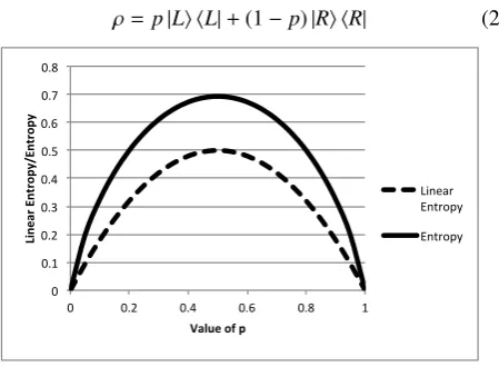
The quantity 1−γ is often called the linear entropy, as it’s the term that comes from the linear expansion of ln(ρ). The linear entropy is a lower approximation to the von Neumann entropy, but is much easier to calculate, since it doesn’t involve diagonalisingρ. In Fig.1 we plot both the von Neumann entropy and the linear entropy as a function ofp, for the state,
ρ=p|Li hL|+(1−p)|Ri hR| (24)
275
0 0.1 0.2 0.3 0.4 0.5 0.6 0.7 0.8
0 0.2 0.4 0.6 0.8 1
Line
ar
Entr
opy/Entr
opy
Value of p
Linear Entropy
[image:6.595.55.280.414.579.2]Entropy
Figure 1: The von Neumann and linear entropies for the state Eq.(24).
For a classical probability distribution, the maximum entropy state is the one with equal probability for any outcome. The quantum analogue of this is a density matrix which is diagonal, and where all the diagonal elements are equal. This state is given (for a Hilbert space of dimensiond) by,
ρmax entropy= 1 d
1 0 · · · 0 0 1 · · · 0
..
. ... ... ...
0 0 · · · 1
=1
d11d (25)
7Note that ifA
i j = Aiδi j then f(Ai j) = f(Ai)δi j. i.e. any function of a
diagonal matrix is itself a diagonal matrix.
where 11dis the identity matrix inddimensions (we will usually drop the subscriptdsince the number of dimensions should be obvious.) It’s easy to see that,
S(ρmax entropy)=ln(d). (26)
which agrees with the classical result for a maximally uncertain 276
state. 277
3.5. Discussion 278
The introduction of states with classical as well as quan-279
tum uncertainty represents a very significant development in 280
the quantum formalism. We can now go ahead and represent 281
a much more general variety of knowledge states, which proba-282
bly better reflect the kind of participants we might encounter in 283
a realistic experiment. 284
However the introduction of these states also gives us a 285
chance to discuss what we think is one of the most powerful 286
a priori reasons for considering quantum models of cognition 287
and decision. At the heart of this argument is the difference be-288
tween classical and quantum uncertainties. Suppose we have 289
a classical system such as a fair coin, where our best descrip-290
tion consists of a probability distribution for the two possible 291
outcomes, head or tails. The probabilistic description reflects 292
the fact that we are uncertain about the outcome of a given 293
coin toss. Classical probability distributions have an associated 294
Shannon entropy, and so classically the uncertainty about the 295
outcome of the coin toss (probabilistic description) is related to 296
a lack of knowledge (entropy) about the state of the system. In 297
other words, classically we have, 298
Uncertainty about outcomes
⇔
Lack of knowledge about state
Suppose we want to build a classical cognitive model of a 299
participant’s preferences; specifically, let’s imagine we want a 300
model of what type biscuit the author will choose to eat from 301
the box he has in front of him, as a reward for finishing this sub-302
section. To simplify matters, suppose there are only two types, 303
milk or dark chocolate. The author professes to be indiff er-304
ent between them currently, and experience (and the number of 305
each kind left in the box) tells us he is equally likely to choose 306
either variety. A classical description of the author’s cognitive 307
state, which aimed to match his behaviour, would have to be 308
a probability distribution which gave equal weight to milk and 309
dark chocolate biscuits. 310
There’s something odd about this though. To be clear, such a 311
descriptionwouldgive the correct statistics for choices. How-312
ever recall our discussion above; this classical probability dis-313
tribution would have an associated entropy, and should be in-314
terpretable in terms of a lack of knowledge about the state. But 315
wait, what information exactly is it that we lack? In the exam-316
ple of a coin toss above, if we toss a coin and ask you to guess 317
heads or tails, there is of course a ‘correct’ answer, a proba-318
bilistic description reflects your lack of knowledge about the 319
onlyknowledgeyou could be lacking here is the author’strue 321
preference for his next biscuit type. In other words, every time 322
you use a classical probability distribution to describe a system, 323
you assume that there is atruestate of the system, that you are 324
ignorant of. This might be ok for coins, but it is far from ob-325
vious that this makes sense for decision makers. For example, 326
according to a classical theory, the author really do have a defi-327
nite preference for my next biscuit, he’s just not telling himself 328
what it is... 329
We don’t want to build a quantum model of biscuits pref-330
erence here, but suppose we represent the author’s preference 331
as the superposition state √1
2(|milki+|darki). This state has
332
the same expected outcomes as the classical probability distri-333
bution, but critically it has zero entropy. That is, for a quan-334
tum superposition, although the best description of the expected 335
measurement outcomes is probabilistic, there is no extra infor-336
mation that it is possible to gain that would improve your ability 337
to predict a choice. In quantum theory, 338
Uncertainty about outcomes
<
Lack of knowledge about state.
For the author’s money, this is one of the most powerful argu-339
ments for using quantum probability theory to model cognition. 340
Now, time for that biscuit. 341
3.6. Summary 342
To recap; we introduced the concept of a density matrix, which can be used to represent a state with both classical and quantum uncertainty. In particular, if we have two different groups of participants, represented by thepure states|P1iand
|P2i, then we can form amixed stateby taking,
ρ=λ|P1i hP1|+(1−λ)|P2i hP2|, 0≤λ≤1. (27)
Hereλgives the relative frequencies of the two types of partici-343
pants in our ensemble. If the two types occur equally frequently, 344
thenλ=12. 345
All of the quantum theory you have encountered before can 346
be rewritten in terms of density matrices, and we gave a few 347
examples of common relations. 348
We discussed the purity and entropy of a density matrix. 349
Pure states always have zero entropy, but density matrices let us 350
think about techniques such as entropy maximisation in quan-351
tum models. 352
Finally we noted that quantum models break the connection 353
between uncertainty and entropy, and this might represent a 354
powerful argument for their use in cognition. 355
4. Noise in the measurements: POVMs
356
4.1. Introduction 357
Designing good experiments is hard. Errors can creep into 358
experiments because of participant quality, but they can also 359
occur because of experimental design. One type of error occurs 360
in studies where the questions have some sort of time pressure 361
associated with them. Participants are forced to rush somewhat 362
through the questions, and as such they sometimes click the 363
wrong box or make other simple errors. Another type of error 364
might occur when studies are very long, and participants loose 365
focus and start giving inconsistent answers. 366
Suppose we wish to model an experiment where we have par-367
ticipants express a preference for one of two alternatives,Aor 368
B, and that these are exhaustive and exclusive alternatives. In 369
an ideal measurement these would be represented by projection 370
operatorsPA =|Ai hA|,PB=|Bi hB|. Suppose instead our mea-371
surement isn’t ideal but, intentionally or otherwise, is subject to 372
some noise. This means some participants who really preferA 373
will select optionB, and vice versa. 374
Let’s see how we might model this. What we want is an operatorEA, whose expectation value in the state|Ai is close to one, but which also has a non-zero expectation value in the state|Bi, and likewise forEB. That is,
hA|EA|Ai=1−, hB|EA|Bi=,
hA|EB|Ai=, hB|EB|Bi=1−.
(28)
Where 0 ≤ ≤ 1 is some small error probability. Let us also assume,
hA|EA|Bi=0, etc. (29)
In the basis{|Ai,|Bi} these operators can therefore be written as,
EA=
1− 0
0
!
, EB=
0
0 1−
!
. (30)
Can we use these operators to describe a measurement process? 375
It is easily seen that they are not projection operators, unless 376
=0 or 1, nevertheless they satisfy the following properties, 377
• They arepositiveoperators, which means they have posi-378
tive eigenvalues. 379
• They arecomplete, in the sense thatEA+EB=1. 380
These properties mean that for any density matrixρ,
0≤Tr(EAρ)≤1 (31)
and
X
i=A,B
Tr(Eiρ)=1 (32)
The quantities Tr(Eiρ) can thus be interpreted as probabilities, 381
and soEA andEBare good candidates to describe a measure-382
ment process. 383
But what measurement process do they describe? Well there are many ways to think about this, but probably the easiest is to note that we can write,
EA =(1−)PA+PB, EB=PA+(1−)PB. (33)
In other words, we can write these operators like,
EA=
X
i
pA(i)Pi (34)
where pA(i) have (loosely) the interpretation of probabilities. 384
So one way to think about these measurements is that instead 385
of performing a measurement PA, we instead perform one of 386
the possible measurementsPiwith some probabilitiespA(i). So 387
these sorts of measurements look like noisy versions of ideal 388
measurements. 389
4.2. POVMs 390
EA and EB together form a specific example of what are 391
known as positive operator valued measures or POVMs for
392
short Busch et al. (1995); Neilsen and Chuang (2000). POVMs 393
are the most general type of measurements that can occur in 394
quantum theory. What we want to do now is present an outline 395
of the general theory of POVM measurements. After this we 396
will go on to discuss some more concrete examples. 397
The most general description of a measurement process in 398
quantum theory is given in terms of a POVM, which is a set of 399
operators{Ei}, that satisfy, 400
• Positivity,hψ|Ei|ψi ≥0, ∀ |ψi ∈H 401
• Completeness,P
iEi=1.
402
The probability that a measurement described byEigives a pos-itive answer is then given by,
p(i)=Tr(Eiρ). (35)
A given POVM can have many different possible realisations. A realisationφiis essentially the operation applied to the state
ρ→φi(ρ), so that,
Tr(φi(ρ))=Tr(Eiρ) (36)
The simplest realisation of a POVM{Ei}probably consists of just taking the operator square roots of theEi, i.e. writing
Ei=Mi†Mi (37)
we have
φi(ρ)=MiρMi†. (38)
The Miare often called ‘measurement operators’. It’s easy to see from this why a given realisation of a POVM isn’t unique. Suppose we use different measurement operators given byM0
i =
U MiwhereUis an unitary operator. Then,
Mi0†M0i =M†iU†U Mi=M†iMi=Ei (39)
so these new measurement operators form a realisation of the same POVM, but,
φ0
i(ρ)=U MiρM†iU
†=
Uφi(ρ)U† (40)
so the final state after the measurement is different in the two 403
realisations. 404
In the rest of these notes we will mostly ignore the issue of 405
multiple realisations, by sticking to the choice Mi =
√
Ei. In
406
practice the appropriate realisation can be determined from the 407
details of the measurement process. 408
The analogue of the collapse postulate in terms of POVMs is simply that if a measurement of the POVM{Ei}yields the outcomei, then the state collapses to,
ρ0= φi(ρ)
Tr(φi(ρ))
= MiρM
†
i.
Tr(Eiρ)
, (41)
where the second equality holds for our simple choice of reali-409
sation Eq.(37) 410
To return to our example above, for the POVM EA, in the basis{|Ai,|Bi}the associated measurement operator will be,
MA =
√
1− 0
0 √
!
, MB=
√
0
0
√
1−
!
, (42)
which is nice and simple. 411
One feature of POVMs that is worth noting is that they rep-resent measurements that are not perfectly repeatable, in the sense that if we measure a variable and find the value xthen immediately measuring the same variable again will not yield the result xwith certainty. This is essentially because for the elements of a POVME2A,EA. Suppose we start with an initial stateρ=diag(1−p,p). If we measure the POVM above and get the outcomeAthen our state collapses to,
ρ0= 1
(1−)(1−p)+p
(1−)(1−p) 0
0 p
!
. (43)
if we now perform another measurement of the POVM then the probability we will get the outcomeAagain is,
Tr(EAρ0)=
(1−)2(1−p)+2p
(1−)(1−p)+p ≤1 (44)
for smallandp<1 this goes as,
Tr(EAρ0)=1−
1−p +O(
2) (45)
so that this POVM measurement is not perfectly repeatable. 412
4.3. Non-Orthogonal Measurements and ‘Maybe’ 413
One interesting property of POVMs, as opposed to a descrip-tion of a measurement process based on projecdescrip-tion operators, is that the elements of a POVM need not be orthogonal. This means that we can have more measurement outcomes than there are dimensions in our Hilbert space. One application of this is where we have a two dimensional set of choices, say Aor B, but more than two possible responses, say “preferA”, “prefer B” and “don’t know”. There are doubtless better ways of mod-elling this situation, but let’s follow this through and see what happens. The states associated with each outcome are given by,
PreferA =|Ai
PreferB =|Bi
Don’t know =√1
2(
|Ai+|Bi)
or √1
2(
|Ai − |Bi)
They have associated projection operatorsPA,PB,P+andP−in
what we hope is an obvious notation. Now these set of pro-jection operators can’t form a description of a measurement, because they are not normalised, i.e.
X
i=A,B,+,−
Pi=2 (47)
but we can easily turn them into a POVM by normalising. The POVM is therefore given by the set,
EA =
PA
2 , EB =
PB
2 , E+=
P+
2 , E−=
P−
2 . (48)
Suppose our state is|+i= √1
2(|Ai+|Bi). Then we can show,
p(A)= 1
4, p(B)= 1
4, p(don’t know)= 1
2. (49)
It turns out this example is not very realistic (e.g. 414
p(don’t know) = 12 always!) but we hope it shows POVMs 415
have potential for modeling this kind of measurement. We will 416
see a better example in the next section. 417
4.4. POVMs for Likert scales 418
Many experimental conditions in psychology involve re-419
questing responses on a Likert scale. Belief and preference 420
strengths are often elicited in this way, but they can be used 421
to measure almost any cognitive variable. 422
Likert scales pose an interesting problem for quantum mod-423
els, because it is somewhat unclear how to approach modeling 424
the corresponding variables. Suppose one is interested in a vari-425
ablexwhich we are going to take to be a belief that some event 426
will happen, say that it will rain tomorrow. One might imagine 427
measuring participant’s beliefs about this event in a number of 428
different ways, 429
1. Do you think it will rain tomorrow? (Yes, No) 430
2. Do you think it will rain tomorrow? (Yes, No, Not Sure) 431
3. On a 1-9 scale, where 1 is certainty of rain, and 9 is cer-432
tainty of no rain, how likely do you think it is that it will 433
rain tomorrow? 434
4. What percentage chance do you think there is of rain to-435
morrow? 436
5. ... 437
It is reasonably clear that these are all measuring the same un-438
derlying cognitive variable, belief in rain tomorrow. However if 439
one assumes that the different response options are orthogonal 440
then they appear to require vastly different dimensional Hilbert 441
spaces, from 2 to 100 (or even an infinite dimensional space 442
if one allows a continuous response option like a slider.) Our 443
challenge is to come up with a unified way of modeling these 444
different response types as arising from a single quantum vari-445
able. There are many way to do this. We will describe one of 446
the simplest8.
447
8An even simpler way is to ignore the issue and assume participants have
Suppose we allow the different responses on the Likert scale to be non-orthogonal. Suppose we use an N point scale, we can take the responses|x=0i =|0iand|x=Ni =|1iand the intermediate responses to be,
|x=ni=cos
nπ
2N
|0i+sin
nπ
2N
|1i (50)
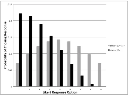
These states give rise to a set of projection operators{Pn}that 448
can be turned into a POVM by normalising. The probabilities 449
that a measurement of this variable will yield one of the re-450
sponses 1-9 for the states|0iand √1
2(|0i+|1i) are shown in Fig
451
2, for the choice of a 9 point response scale. Note that there is
0 0.05 0.1 0.15 0.2 0.25
1 2 3 4 5 6 7 8 9
Pr
ob
ab
ili
ty
o
f C
ho
si
ng
Re
sp
on
se
Likert Response Op7on
[image:9.595.324.542.238.398.2]State ~ |0>+|1> state = |0>
Figure 2: Probabilities for each of the 1-9 options on a Likert scale assuming the POVM based on Eq.(50).
452
obviously some spread in the choices, however if the true state 453
is|0i, say, then the probability of choosing either 1,2 or 3 on the 454
scale is almost 63%. 455
There are other, perhaps better ways of modeling Likert scale 456
type judgments in quantum theory, in particular this approach 457
rapidly looses its value as the number of responses becomes 458
larger. Nevertheless we hope this semi-realistic example is use-459
ful in setting out where POVMs can be used in practice. 460
4.5. Order effects in noisy measurements
461
An important question is whether noise in the measurement 462
process spoils the quantum features of that measurement. One 463
example of such a quantum feature is order effects in survey 464
designs (Wang et al., 2014), so we will briefly look at whether 465
noise in the measurements spoils order effects. This is covered 466
in more detail in Yearsley and Busemeyer (2015). 467
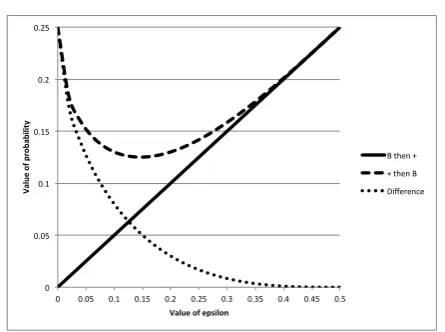
A striking simple example of an order effect is to consider an initial state|Aiand two possible projective measurements, PB
direct access to the probability Tr(Pxρ). This is frequently done in quantum
models. However this is problematic for two reasons; first this probability is an expectation value that only makes sense for an ensemble of systems, which requires that participants have not a single belief state but a whole collection that they can query. In other words, this is not actually quantum theory of a single belief state anymore. Second, because this measurement is not modeled in a proper quantum way, it is unclear what happens if we ask participants to make sequential Likert scale type judgements. What does the state collapse to after the first judgment?
onto the state|BiandP+onto the state, √1
2(|Ai+|Bi). It is easy
to see that (working for the rest of this subsection in the basis
{|Ai,|Bi}),
p(+and thenB)=Tr(PBP+ρP+)
=Tr
0 0
0 1
! 1 2
1 2 1 2
1 2
!
1 0
0 0
! 1 2
1 2 1 2
1 2
!!
=Tr
0 0
1 4
1 4
!!
=1
4
(51)
Whereas,
p(Band then+)=Tr(P+PBρPB)
=Tr
1 2
1 2 1 2
1 2
!
0 0
0 1
!
1 0
0 0
!
0 0
0 1
!!
=Tr
0 0
0 0
!!
=0.
(52)
This striking result arises from the fact that [PB,P+] ,0. So 468
what happens if we replace this set of ideal measurements with 469
a POVM? 470
We let’s replace the projection operators with the following
9,
PB→EB=
0
0 1−
!
P+→E+=
1 2
1−2
2 1−2
2 1 2
! (53)
These have associated measurement operators,
MB=
√
0
0
√
1−
!
M+=
√
1−+√
2
√
1−−√e
2
√
1−−√e
2
√
1−+√
2
(54)
Now we can see that,
p(+and thenB)=Tr(EBM+ρM+)
=1
4
1−2(1−2)√
√
1− (55)
and
p(+and thenB)=Tr(E+MBρMB)
=
2
(56)
We plot these results against the value ofin Fig.3. The re-sults are interesting. The key is that the difference in the values of the probabilities, ie
δ=p(+and thenB)−p(+and thenB) (57)
9Readers are encouraged to convince themselvesE
+is reasonable. Either start withPBand rotate throughπ/4, or consider a combination ofP+andP−
as in Eq.(34).
(plotted as the dotted line) decreases sharply with increasing, 471
i.e. with increasing noise. Note however that the value of is 472
interpretable in terms of the ‘error’ probability of the measure-473
ment. Realistic experiments would probably have values of 474
in the range 1-5% (as found in Yearsley and Pothos (in press)), 475
and so order effects are still likely to be visible in such experi-476
ments, although they might appear smaller than you might have 477
expected.
0 0.05 0.1 0.15 0.2 0.25
0 0.05 0.1 0.15 0.2 0.25 0.3 0.35 0.4 0.45 0.5
Va
lu
e o
f p
ro
ba
bi
lit
y
Value of epsilon
B then + + then B
[image:10.595.321.544.181.347.2]Difference
Figure 3: p(Band then+), p(+and thenB), and their difference, plotted against.
478
We don’t have space here to pursue this further, but it is clear 479
that small amounts of noise will still allow order effects to be 480
observed, even though very large amounts of noise rapidly kill 481
off such effects. This has important implications for studies 482
looking for these effects in the wild (Wang et al., 2014). 483
4.6. Summary 484
We have shown that the description of measurements in 485
quantum theory can be generalised to non-orthogonal sets of 486
measurements. These POVM type measurements can be used 487
to describe noisy realistic measurements, where even partici-488
pants with a definite knowledge state may not make completely 489
predictable decisions. They can also be used to model situations 490
where there are simply more possible choices than orthogonal 491
states in the space. 492
We mentioned that one useful way to think about POVMs was as averages over a set of projective measurements, e.g.
EA=
X
i
pA(i)Pi (58)
where the{Pi}are a complete and orthogonal set of projection operators and thepA(i) are positive numbers such that,
X
A
pA(i)=1. (59)
which ensures the POVMs are normalised. 493
POVMs are likely to be a very important tool as we strive 494
to make the predictions of the quantum models more accurate. 495
They are also particularly relevant if an experimental set up in-496
volves asking participants the same questions repeatedly, see?
497
5. Noise in the Evolution: CP Maps
499
5.1. Introduction 500
The final type of noise we will consider is noise in the evo-501
lution of the state. In a typical experiment we manipulate the 502
cognitive state of a participant by presenting some kind of stim-503
uli. Although we might have good control over the stimuli we 504
present, we have much less certainty about how particular par-505
ticipants respond to these stimuli. In addition, we usually as-506
sume that different preferences and beliefs are more or less in-507
dependent of one another, so that, e.g., a model of chocolate 508
biscuit preference can consider this belief state as an isolated 509
system, independent of, e.g. preference for tea or coffee. 510
In reality, things are not this simple. We therefore need more 511
realistic models of evolution that can help us answer two ques-512
tions; 513
1. What effect does the interaction between different be-514
liefs/preferences have on the evolution of a cognitive state? 515
2. How do we model evolution when we are unsure about the 516
effect of a stimuli on a particular participant? 517
It will turn out that these two questions have essentially the 518
same answer. In addition an important motivation for consider-519
ing noisy evolutions turns out to be the following question, 520
3. How do we model evolutions that are irreversible, or that 521
cause a general initial state to tend towards some final fixed 522
state which is independent of the initial one? 523
This question arrises because the usual unitary evolution we 524
consider is reversible, ie for any unitary evolutionU(t)=e−iHt 525
there is another unitary evolution given by U†(t) such that 526
U(t)U†(t) = U†(t)U(t) = 1. There are of course many situ-527
ations in cognition where we might wish to model evolutions 528
that are (effectively) irreversible, eg decays. This is particularly 529
apparent when we cause a cognitive state to evolve by present-530
ing some stimuli, e.g. some extra information, whose effects 531
we can’t undo. 532
Again, somewhat remarkably, we will find that the answer 533
to question 3 is the same as the answers to questions 1 and 534
2. We will also find that this way of incorporating noise into 535
cognitive models has some very profound consequences for the 536
‘quantum-ness’ of the systems under study. 537
5.2. CP Maps 538
Generally speaking, in quantum theory noisy evolutions are 539
motivated by considering a system of interest S which inter-540
acts with some other less well controlled system which we 541
call an environment E. We will follow the same reasoning, 542
although it’s reasonable to have concerns about how well the 543
physics/cognition analogy works here. In the end though the 544
key point of this subsection is that there is a standard form for 545
these noisy evolutions which guarantees that they make mathe-546
matical sense. In practice we just pluck noisy evolutions out of 547
thin air to do a particular job, our only concern being that they 548
match this standard form. However it’s useful to have some 549
idea about where they come from10. 550
The idea is that we want to study the systemS which inter-551
acts with an environmentE about which we have little or no 552
interest in or information on. What one does then is to specify 553
the dynamics of the joint system+environment, including in-554
formation about the evolution and initial states to arrive at a de-555
scription of the density matrix of the whole,ρS+E. This density
556
matrix contains information about the environment, which we 557
don’t want, so to get at a description of just the system we per-558
form an operation called apartial trace, where we sum over the 559
environmental degrees of freedom, essentially throwing away 560
the information we don’t want, to leave us with an effective 561
description of the dynamics of the system only in terms of a 562
reduced density matrixρS. 563
We are interested in the effect this has on the master equation for the system alone, i.e. the evolution equation for the reduced density matrixρS. For the complete density matrix ρS+E we
have,
∂
∂tρS+E=−i[HS+E, ρS+E] (60)
whereHS+Eis the joint Hamiltonian of the system plus
envi-ronment. When we perform the partial trace to remove the en-vironmental degrees of freedom this becomes,
∂
∂tρS =−i[HS, ρS]+LρS (61)
whereLis a super-operator which encodes the extra dynamics that come from the system-environment interaction. The most general form this equation can take is the so-called ‘Lindblad’ form (Lindblad, 1976),
∂
∂tρS =−i[HS, ρS]
+X
k
LkρSL†k−
1 2L
†
kLkρS −
1 2ρSL
†
kLk
! (62)
where{Lk}are a set of operators called the ‘Lindblad’ operators, 564
which model the effect of the environment. 565
The key feature of evolution according to the Lindblad equa-566
tion is that it preserves the properties of the density matrix 567
which are important if it is to describe a real cognitive system. 568
The most important (in the sense of difficult to achieve) prop-569
erty ispositivity, which recall means that all the eigenvalues of 570
ρare non-negative. For this reason master equations of the form 571
Eq.(62) are known as ‘Completely Positive’ or CP-maps11. In
572
the next sections we will consider a number particularly useful 573
CP-maps, designed to model specific types of evolution. 574
5.2.1. Some Extra Detail 575
We add a few extra points here for interested readers. 576
10It’s worth noting that this will be pretty wooly. The full mathematical
treatment is complex and irrelevant for usage we want to make of the formalism.
11Actually Eq.(62) has an additional property not needed to preserve the
properties of the density matrix, which is that it is continuous in time. Evo-lutions of the form Eq.(62) are therefore only a subset of possible CP-maps.
In the derivation of Eq.(61) we assume that we can separate out the system and environmental degrees of freedom in the system. So we can write the total Hilbert spaceH =HS⊗ HE. We can therefore choose a basis for the Hilbert space which consists of tensor products of basis vectors from the system and environment, i.e.
φi j E
=|Sii ⊗
Ej
E
, where{|Sii}form a basis forHS, and likewise for the environmental degrees of freedom. The partial trace over the environmental degrees of freedom is therefore defined as,
TrE(A)=
X
j
D
Ej A
Ej
E
(63)
and the reduced density matrix for the system alone is given by,
ρS =TrE(ρS+E). (64)
A couple of further points to note. First, most derivations of Eq.(61) for real systems assume that the initial density matrix can be factorised as
ρS+E(t=0)=ρS(t=0)⊗ρE(t=0). (65)
In other words the assumption is that the system and environ-577
ment were independent to begin with, at timet =0. This can 578
have some funny effects on the dynamics. For example, one of 579
the features of noisy evolutions is that they tend to kill of en-580
tanglement between different parts of the system. However if
581
you take two systems and allow them to interact, they will tend 582
to become entangled with each other. These models of noisy 583
evolutions can therefore have some funny behaviour at short 584
times, that results from assumptions made about the initial state 585
to simplify the analysis. 586
Another point to note is that in order to make the transition 587
from Eq.(60) to Eq.(61) tractable one often has to make sim-588
plifying assumptions about the dynamics. Typical assumptions 589
are that the interaction between the system and environment is 590
weak, and also that it is Markovian. Thus many explicit models 591
of noisy evolutions are Markovian. If you have good reason to 592
believe the system you are trying to model does not have this 593
property, you should be extra careful in your choice of CP map. 594
Finally, if you are interested in seeing how a derivation of 595
the master equation for a real system/environment interaction 596
proceeds, I strongly recommend the paper by Halliwell (2007), 597
for a simple introduction. This gives a simplified derivation of 598
the master equation for quantum Brownian motion, that is, the 599
dynamics of a system coupled to a thermal environment. The 600
full blown analysis can be found in the classic paper by Caldeira 601
and Leggett (1983), and also in Breuer and Petruccione (2006); 602
Hu et al. (1992). A nice introductory tutorial can be found in 603
Kryszewski and Czechowska-Kryszk (2008). 604
5.3. A CP-Map for Irreversible Evolutions 605
In this section we want to introduce a tractable example of a 606
master equation we could use to describe a real cognitive sys-607
tem. The example we will discuss is a simple two-level system 608
{|1i,|2i}, that might be used to model a binary variable. For the 609
rest of this section we’ll work in this basis. 610
Now a good model for the noisy evolution of such a sys-tem is given by the so-calledQuantum Optical Master Equation (QOME), which describes the evolution of a two level system interacting with a thermal (i.e. random) system of other sys-tems. The dynamics of this system are described by a master equation of the form Eq.(62) with,
L1=a
0 1
0 0
!
, L2=b
0 0
1 0
!
(66)
and with the specific choice a =
√
ωN, b = √ω(N+1)
611
whereωandNare constants. 612
However the full dynamics of the QOME is complex (For a 613
full solution see Yu (1998); Breuer and Petruccione (2006).). So 614
instead of considering the full dynamics of a system interacting 615
with an environment, what we will do here is to use a special 616
case of this master equation to solve an important problem in 617
quantum models of cognition - how do we model an irreversible 618
evolution? 619
To keep things simple, we will specialise to the following 620
situation: We have an initial state |ψ0i = √12(|1i +|2i), and
621
we want to imagine evolving the state in an irreversible way, 622
maybe by giving the participants new information that cannot 623
be taken back, so that the state tends towards|1i. Unitary evo-624
lution won’t work here, first since it’s reversible, and second 625
since evolving for long enough could cause the state to ‘over-626
shoot’ and move back towards|2i. 627
It turns out that one solution to this problem is given by a special case of the QOME, with a = √γ some constant and b=0, that is,
∂
∂tρ=γ LρL
†−1
2L
†Lρ−1
2ρL
†L
!
(67)
withL = 0 1
0 0
!
, and we’ve assumed there is no unitary part
to the evolution. The solution, for the initial condition given above, is,
ρ(t)= 1−
1 2e
−γt 1 2e
−γ2t
1 2e
−γ2t 1 2e
−γt
!
(68)
As we can easily see, the solution tends to|1i at large times, 628
and it doesn’t overshoot. |1iis therefore afixed point of the 629
evolution. This solution therefore describes a state evolving 630
towards|1i, and getting there asymptotically. Solutions for de-631
cays towards other states can be obtained by applying unitary 632
transformations to the Lindblad operators. 633
One interesting feature of this evolution is that it does not 634
preserve the purity of the state, and by extension also the en-635
tropy. Typically the entropy initially increases, before decreas-636
ing again as the state tends to the known final state. The reason 637
for this is subtle but is essentially due to the fact that this system 638
is not closed but is modeled as interacting with a much larger 639
system. The total entropy of system plus environment will al-640
ways increase, as it should. We plot the behavior of the entropy 641
and purity in Fig.4. 642
In summary then, this particular example of a master equa-643
0 0.1 0.2 0.3 0.4 0.5 0.6 0.7 0.8 0.9 1
0 5 10 15 20 25
Va
lu
e
Time (Dimensionless Units)
Value of Entropy, Purity and ρ_22 as func>ons of >me
[image:13.595.54.273.79.225.2]Purity ρ_22 Entropy
Figure 4: Evolution of the entropy, purity and value ofρ22(t) for the evolution
in Eq.(68).
which are common place in the lab, but impossible to model via 645
unitary transformations. There are many other possible master 646
equations for modeling this sort of evolution, but they all have 647
in common that they represent noisy, non-unitary evolution. 648
5.4. A CP-Map for Uncertain Stimuli: The Montevideo Master 649
Equation 650
In this section we want to consider a second type of noisy 651
evolution, which is not so readily interpretable in terms of a 652
system/environment interaction. However we shall see that it 653
too can be modeled in terms of a master equation of Lindblad 654
form. 655
Suppose we wish to model the evolution of a system caused 656
by the presentation of certain stimuli. Suppose we can present 657
our stimuli in a continuous manner, so it could be that the 658
change in the cognitive state depends on the length of time 659
for which the stimuli are presented. Alternatively it could be 660
that the stimuli are discrete, but individually weak, so that pre-661
sentation of multiple stimuli can be closely approximated by a 662
continuous in time master equation like Eq.(61). Either way, 663
suppose the stimuli are fixed, but their effect on the participants 664
is unknown. We might be able to assume that the effect of the 665
stimuli is on average to produce a shift in a certain direction, 666
but the size of that shift is unknown. This is equivalent to say-667
ing that we have a definite evolution but we are unsure, for each 668
participant, how long that participant’s state is evolved for. 669
Specifically, we will assume that the effect of evolution of a state for a time t is not to produce the change ρ(0) →
e−iHtρ(0)eiHtbut rather,
ρ(t)=
Z
dspt(s)e−iH(t+s)ρ(0)eiH(t+s) (69)
where pt(s) is a probability distribution centered around 0, re-670
flecting the distribution of ‘evolution times’ for our participants, 671
and we have assumed the underlying evolution about which we 672
are uncertain is unitary. If pt(s) = δ(s) we recover standard 673
unitary evolution. We have allowed this probability distribu-674
tion to depend on talso to reflect the fact that the uncertainty 675
in the evolution time, i.e. the width of pt(s), might depend on 676
the time evolved for, so that longer average evolution times are 677
associated with larger uncertainties. 678
We want to be able to represent this evolution in the form of a semi-group12, in other words, ifρ(t)=Lt(ρ(0)), then we want,
Lt(Ls(ρ(0)))=Lt(ρ(s))=ρ(t+s)=Lt+s(ρ(0)). (70)
In other words,Lt· Ls=Lt+s. Writing this in terms of Eq.(69) we see that we can express this evolution in one of two ways,
ρ(t1+t2)=
Z
dspt1+t2(s)e
−iH(t1+t2+s)ρ(0)eiH(t1+t2+s) (71)
or
ρ(t1+t2)=
Z
ds2pt2(s)e
−iH(t2+s2)ρ(t
1)eiH(t2+s2)
=Z ds1ds2pt2(s2)pt1(s1)
×e−iH(t1+t2+s1+s2)ρ(0)eiH(t1+t2+s1+s2)
=Z dsdzpt2(s−z)pt1(z)
×e−iH(t1+t2+s)ρ(0)eiH(t1+t2+s)
(72)
Eq.(71) and Eq.(72) are equivalent if,
pt1+t2(s)=
Z
dzpt1(z)pt2(s−z) (73)
which constrains the possible form forpt(s). One natural choice is the following,
pt(s)=
r
1
πσte
−s2
σt (74)
whereσ > 0 is some constant. This is easily seen to be nor-malised and to obey Eq.(73). Note also that,
lim
t→0pt(s)=δ(s) (75)
in the sense of distributions. (δ(s) here is the Dirac delta func-679
tion13.)
680
We want to show that this evolution can be written in the form of a master equation. We start with Eq.(69), differentiate both sides with respect tot, and use the very useful property, for smallt14,
pt(s)=
r
1
πσte
−s2
σt =δ(s)+σt
4 δ
00(s)+... (76)
to obtain,
∂ρ
∂t =−i[H, ρ]−
σ
4[H,[H, ρ]]
=−i[H, ρ]+σ
2(HρH− 1 2H
2ρ−1
2ρH
2)
(77)
12All physical evolutions have to be expressible in terms of semi-groups,
which means that the product of two evolutions is also an evolution. If an evolution also has an inverse, then it is representable as a group, not just a semi-group. Unitary evolutions have this form.
13Defined byR∞
−∞dxδ(x−x0)φ(x)=φ(x0) for any smooth functionφ.
14Despite the fact that this expansion is very useful, we know of very few
places where it is discussed. The one reference we have for this is page 703 of Kleinert (2006), but this is a horrific textbook on path integral methods in quan-tum theory, and hardly a good go to formula book. If in doubt, just integrate this expression against a smooth test function and you can see why the result is true.