Computational estimation of scene structure through texture gradient cues

City, University of London Institutional Repository

Citation: Tyler, C. W. & Gopi, A. (2017). Computational estimation of scene structure

through texture gradient cues. Paper presented at the IS&T International Symposium on

Electronic Imaging Science and Technology 2017, 29 Jan - 2 Feb 2017, California, USA.

This is the published version of the paper.

This version of the publication may differ from the final published

version.

Permanent repository link: http://openaccess.city.ac.uk/19332/

Link to published version:

http://dx.doi.org/10.2352/ISSN.2470-1173.2017.14.HVEI-138

Copyright and reuse: City Research Online aims to make research

outputs of City, University of London available to a wider audience.

Copyright and Moral Rights remain with the author(s) and/or copyright

holders. URLs from City Research Online may be freely distributed and

linked to.

C

E

S

S

T

G

C

Christopher W. Tyler and Ajay Gopi Smith-Kettlewell Eye Research Institute

San Francisco California USA.

Abstract

Analyzing the depth structure implied in two-dimensional images is one of the most active research areas in computer vision. Here, we propose a method of utilizing texture within an image to derive its depth structure. Though most approaches for deriving depth from a single still image utilize luminance edges and shading to estimate scene structure, relatively little work has been done to utilize the abundant texture information in images. Our new approach begins by analyzing the two cues of local spatial frequency and orientation distributions of the textures within an image, which are used to compute the local slant information across the image. The slant and frequency information are merged to create a unified depth map, providing an important channel for image structure information that can be combined with other available cues. The capabilities of the algorithm are illustrated for a variety of images of planar and curved surfaces under perspective projection, in most of which the depth structure is effortlessly perceived by human observers. Since these operations are readily implementable in neural hardware in early visual cortex, they therefore represent a model of the human perception of the depth structure of images from texture gradient cues.

1 Introduction

Recovering depth information from 2-D images is a basic problem for computer vision which has profound applications in object identification, scene reconstruction, and scene understanding. As stated in the Gibsonian ecological theory of development, our natural ability to perceive the world in 3-D is essential for us to process our environment and for our survival [1]. Embedding our capability to visualize the world into a computer involves challenging problems, but can be useful in computer perception and analysis. Most work on recovering 3D information involves using either multiple images or stereo cues to recreate depth, with relatively less emphasis being placed on monocular cues. As we humans perceive the world through smoothly combining monocular cues (shading, occlusion, relative size, defocus, haze, texture, etc.) with stereo cues (disparity), these monocular cues also play a huge part in our perception [2].

2 Stereo Cues

In stereopsis, each eye receives a slightly different view of the world and the disparity between the views is used to perceive 3-D [3]. Disparity is the misalignment between the two views based on the shifted views in the left eye and right eye of the same environment. Through triangulating the angles of view and disparity, it is possible to see the relative distance between objects in high precision. However, the vast majority of images employed in computer vision, and a large proportion of medical images, are single images of relevant objects without stereoscopic information.

3 Monocular Cues

Aside from common disparity, humans use a large array of monocular cues such as shading, defocus blur, motion parallax, perspective, occlusion, texture gradients, etc. For example, in the case of occlusion, when one object blocks another, the blocked object must be farther away. This allows humans to understand the relative ordering of objects in visual space. Shading also performs a key role in depth perception, as the illumination reflected from objects can also help identify depth [4]. Most monocular cues, however, require contextual information, and they must be assessed in global relation to each other across the image space.

4 Textural Approach

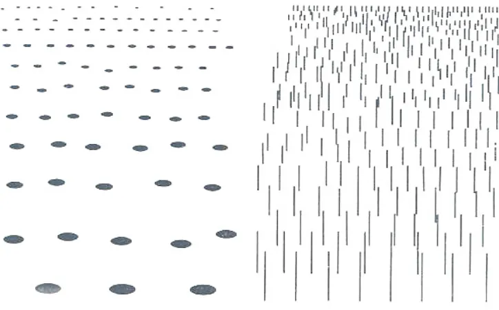
As brought out by Gibson [1], the texture gradients in images of textured objects provide a primary cue to ascertain the depth structure of object in natural images. When a grass field is viewed, the image of the nearby texture is much coarser than the farther texture. Thus, the change in detail within the texture can be used to determine relative distance of different regions of the same texture. Gibson did not, however, actually study the kinds of neural computations that would be needed to extract the shape information from natural textures. Despite his emphasis on the natural world, he restricted his investigations to artificial constructions of simple texture gradients, as in the examples in Figure 1.

dimensions or organization: (1) The texture in the left panel is a semi-regular texture, whereas that in the right panel is irregular but statistically self-similar. (2) The texture in the left panel is sparse, whereas that in the right panel is dense. (3) The texture in the left panel is locally isotropic, whereas that in the right panel is locally oriented. (4) Conversely, the texture in the left panel is globally anisotropic (with the elements arranged in approximately horizontal lines), whereas that in the right panel

is isotropic (though randomized). (5) The texture in the left panel is a flat 2D texture, whereas that in the right panel is a thick 3D texture. This last feature has the consequence that the slant of the one in the left panel can be assessed from the distortion of the individual elements, whereas the elements in the right panel are locally frontoparallel, requiring a global analysis of the relationships among the elements to assess the slant.

Figure 1. Two examples of simple artificial texture gradients from Gibson (1955). Left panel: linear gradient of a regular sparse texture. Right panel: linear gradient of an ergodic dense 3D texture.

A final aspect of texture gradients that deserves comment is that the retinal gradient of texture density is defined with respect to the angle of the visual rays to the eye. However, a linear gradient of uniform texture in the world does not project to a uniform texture gradient on the retina due to the curvature of the retina. This transform is complex and can be broken into two aspects, size and shape. To the extent that the nodal point of the eye (roughly, the pupil) is in the surface of the sphere defined by the shape of the retina, the optical transform from the world to the eye is a stereographic transformation, which has the property that frontoparallel circles in the transform to circles everywhere on the retina. Although this simple description does not apply so well to other geometric figures, it does mean that orientational properties are roughly preserved through the stereographic transform. Relative sizes in this projection are not, however, preserved, but scale inversely with the cosine of the angle of projection relative to the visual axis. An early attempt to compute the texture cue [4] used only the size cue of peak horizontal spatial frequency. A more

represent as well as to the sparseness of the edge information. It is therefore timely to develop a more comprehensive algorithm for 3D shape from texture, taking into account both the orientation and scaling modulations of the texture due to the 3D shape of the textured surfaces, for both isotropic and anisotropic textures, with provision for transitions from one texture to another both within and between objects.

In this paper, we propose a way of using textural cues, to recover depth information from single-frame still images. Texture, is defined here as any surface pattern that is

self-similar over translation up to some scale of analysis, namely, the size of the window within which the n-gram statistics are evaluated [8]. To put it simply, the histogram of any feature in a texture, should be locally similar between adjacent blocks. It is assumed in this report that viewpoint for viewing the image/scene is relatively close, so that a uniform physical texture projects with a texture gradient (perspective transform) into the picture plane. Failures of self-similarity are assumed to imply the transition from one distinct texture to another, as will frequently occur at the boundaries between objects.

5 Methodology

5.1 Assumptions

The primary assumption of the approach is that the texture of a given natural object to be reconstructed is homogenous, or in statistical terms ergodic. That is, it does not need to be a regular repeating pattern, but has to have the property specified above,

that the nth-order histogram of n-gram statistics for any local patch of texture is similar within some statistical criterion to any other patch of the texture. Other depth cues that might introduce non-structural changes in the image of the texture, such as shading cues, are assumed to be absent.

5.2 Approach

In this method, we separate the image into overlapping blocks, calculate the spatial frequencies in every block and change in frequency, f (slant, k) with respect to adjacent blocks. Under the assumptions of the perspective transform of an eye viewing a world, a uniformly slanted surface should show a decrease in size, s, inversely with distance, d, such that 𝑠 = 𝑘/𝑑, where 𝑓 = 1/𝑠 , and thus distance is proportional to spatial frequency scaled to a constant for any given slant (k). For a linear slant in perspective projection, we know that the spatial frequency scales with distance such that 𝑓)/𝑑)= 𝑓*/𝑑* . We also know

that the slant is given by 𝑘 = 𝑑*− 𝑑)/𝑝*− 𝑝), where 𝑝* and 𝑝₎ are two block positions. Thus by substituting 𝑑_*= 𝑑). 𝑓*/ 𝑓), it follows that 𝑘 = 𝑑)∗ (𝑝*− 𝑝))/(𝑓*/ 𝑓)− 1).

Since the image frequencies can be found and the block positions are specified by the algorithm, assigning an arbitrary 𝑑) value allows the slantvalue at each location of the image to

be calculated. Using the slant value, we can derive the directional change in depth at every given sampling point of the image, which is integrated to create a depth map with one free parameter of its absolute distance. The base depth values are obtained from the frequency map, using the perspective assumption that higher frequencies are farther away.

To derive the frequency values at each block of the image and form a depth map, we use a log-polar subsampling procedure on the block Fourier Transforms.

5.2.1 Extraction of Spatial Frequencies

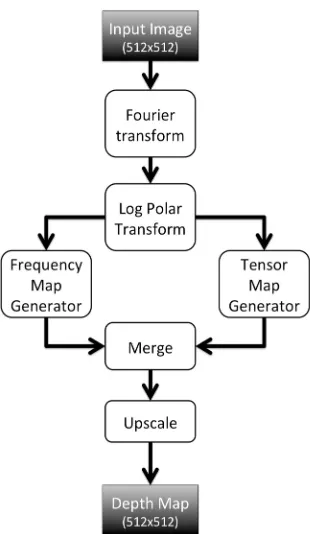
The following is a detailed explanation of every stage of the process as shown in Figure 2. First, the program divides the image into overlapping subregions and applies a Gaussian fade

to each block (of specified size) to eliminate edge artifacts., sampled every half width of a block to provide for the block overlap. Parametric comparisons are then run across blocks, resulting in 𝑛 − 3 comparisons, 𝑛 being the number of indices.

Then, the 2D Fourier Transform is applied to each block of the image. The 2D Fourier Transform decomposes an image into its sinusoidal components, thus showing its spatial frequency

composition, forming a frequency map of the information in the image block (See Figure 2).

5.2.2 Conversion to Log-Polar Plane

Figure 3Error! Reference source not found.B shows a 3D plot of the Fourier amplitude of a typical natural image (from [4]) illustrating its characteristic approximation to a 1/f fall-off

in amplitudes at all orientations (where f = ||u,v||). To focus the analysis on local variations from this fall-off property, the Fourier amplitudes in our 2D Fourier analysis were first multiplied by f to normalize them against this kind of fall-off.

A B

Figure 3: Extraction of spatial frequencies. A: Rationale for 1/f frequency normalization based on typical 2D Fourier energy distribution for natural scenes (from [2]). B: Depiction of the block Fourier transform operation.

The next operation is to run a log-polar transform of the matrix containing the spatial frequencies using custom code, as shown Figure 1. In this transform, the radius (distance with center as origin) and theta (angular change with center as origin) is derived for every pixel in the Fourier image utilizing the

equations 𝑋 = 𝑅 ∗ 𝑐𝑜𝑠 (𝜃) and 𝑌 = 𝑅 ∗ 𝑠𝑖𝑛 (𝜃). By mapping into the log-polar plane, the shift in frequency of the amplitude structure in the Fourier plane is converted to Cartesian coordinates., such that each block of the image produces a pattern of frequencies in the log-polar plane.

Figure 1: Conversion to log polar plane

5.2.3

A primary texture cue to object distance is the peak spatial frequency of the texture, which increases with distance. Using the log polar matrices, the frequency map is derived as shown

in Figure 5Error! Reference source not found.. The Fourier energy is averaged over orientation and the peak frequency of each block is computed and set as the characteristic frequency for each block. The inverse of this frequency is stored in the

32 x 32

32 x 32

32 x 32

Or

ie

nta

tio

frequency map, such that the higher frequencies (close to black) indicate farther and the lower frequencies (close to white) indicate nearer.

Figure 5: Creation of block spatial frequency map

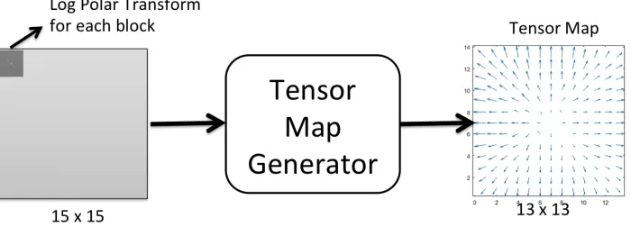
5.2.4 Extraction of the Shifts in Spatial Frequency

To derive the tensor map of the 2D frequency gradient, he predominant frequency and orientation shift between adjacent blocks is measured by cross-correlation between adjacent log-polar blocks, specified mathematically by _>== 𝑓 ∗ (𝑡)𝑔(𝑡 + 𝜏)𝑑𝜏. Since the pattern of Fourier frequencies within a given texture is similar at all locations (by the translation self-similarity property of the texture definition), the peak shift of the cross-correlation will define the gradient of change in

frequency. Thus, the cross-correlation itself shows the frequency or orientation difference as a peak shift from the center of the cross-correlation. Depending on the shift intensity and direction, one can determine where the gradient is going from coarse to fine, and vice versa. The two-dimensional (spatial frequency and orientation) shifts between log-polar blocks may then be plotted as a tensor map as shown in Figure 6.

Figure 6: Extraction of the spatial frequency gradients.

To eliminate unnecessary DC frequencies, which would degrade the peak-shifting assessment, the mean is removed from the image block. By running the block analysis both vertically and horizontally, the shift in spatial frequency throughout the image is captured in two dimensions. The estimated frequency and orientation shift is graphed in vector

format as tensor map (see Figure 6), mapping the gradient changes throughout the image. Transitions from one texture to a different texture may be signaled by demarcating a texture boundary if the peak cross-correlation falls below a criterion correlation level, such as 0.5.

To this point, we have been treating gradients as involving a frequency variation. There is a subtlety here, however, since this logic depends on the form of perspective involved. In parallel (isometric) perspective there is no frequency variation with distance, whereas natural images always have some degree of convergent perspective. This means that any slanted surface will have some degree of frequency gradient to it, which is our primary cue to depth from texture.

However, there is also an overall frequency compression resulting from a texture gradient d(x,y) as a function of the angle of view to the line of sight, or foreshortening, implying that the frequency estimate for a uniform gradient will show a degree of frequency compression proportional to the steepness of the gradient.

The use of the frequency map per se is still suboptimal, therefore, as it does not take into account the frequency compression resulting from a texture gradient as a function of

the angle of or foreshortening. The frequency coding principle treats such compression for oblique gradients as a region of uniformly greater distance. The gradient approach can correct for the lack of a gradient estimate in the frequency image, but it needs to also provide a correction to the frequency estimate based on the presence of the local gradient (Figure 7).

Thus, the frequency information is proportional to distance d

with an arbitrary scaling factor defined by the nature of the texture, fT, with an additional term defined by the absolute value

of the surface gradient, |f(x,y)’|. Since the same degree of foreshortening is provided by both a positive and a negative slant to the line of sight, the sign of the slant is ambiguous in terms of its effect on frequency, and is given by its absolute value: F(x,y) = fT / (d(x,y) + k.|d(x,y)’| ). Thus, in order to

compensate the frequency estimate of distance D for the foreshortening effect, we need to subtract the absolute value of the local frequency gradient from it: d(x,y) = fT/ F(x,y) -

k.|d(x,y)’|.

Figure 2: Creation of final depth map

6 Results

The following figures provide a compilation of some of the 2D depth images that were analyzed through the program. In the following depth maps, white represent absolute closeness and

dark represents absolute distance (scale bar). These results reinforce the notion that texture is a strong perceptual cue that can be used to extract depth information from single 2D depth images.

6.1 Simple artificial images

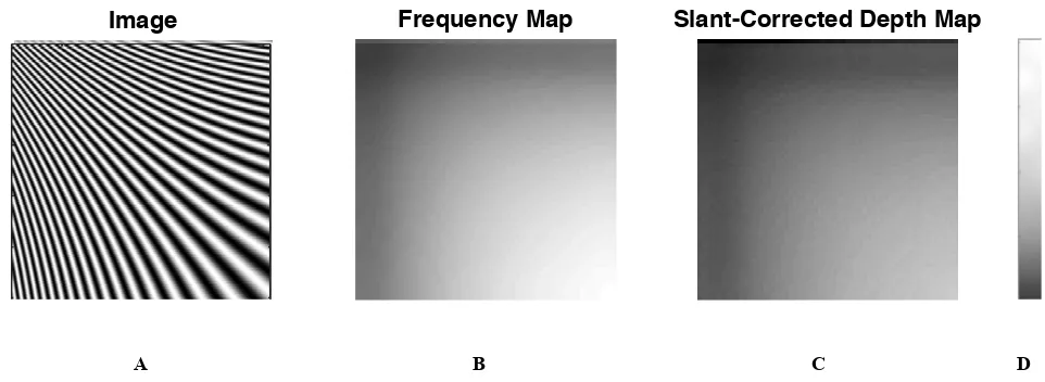
Figure 7 is a good example of a simple anisotropic frequency gradient validating the primary algorithm by showing how the

not require the assumption of local isotropy of the texture, but works equally well for anisotropic texture.

A B C D

Figure 7. A. Oblique frequency gradient in a one-dimensional texture. B. Frequency map. C. Slant-corrected depth map. D. Scale bar: brightness represents estimated distance, with farther coded as darker as indicated by the depth bar at right.

Figure 8 is a more complex one-dimensional gradient (‘Fission by Bridget Riley, 1962) based on a two-dimensional dot pattern, illustrating that the algorithm can handle regular isotropic texture gradients. Notice also that the depth reconstruction

captures the uniformity of the gradient in the vertical direction, and also the subtle difference between the longer gradient on the left side and the shorter gradient on the right side, which is difficult perceive with the human eye without careful scrutiny.

A B C D

Figure 8. Two-dimensional texture with an anisotropic, one-dimensionally modulated gradient. Coding as in Figure 7.

6.2 Complex artificial images

Figures 9 and 10 are examples of complex texture gradients for which the approach was able to detect the gradient changes in all directions. In Figure 9, the structure is given mainly by

texture gradients, while in Figure 10 the main changes are in texture orientation. Bothe are captured well by the algorithm, illustrating the flexibility of the algorithm capabilities.

A B C D

Figure 9. Complex rotational frequency gradient. Coding as in Figure 7.

A B C D

Figure 10. Complex orientation gradient – ‘Fall’ by Bridget Riley (1963). Coding as in Figure 7.

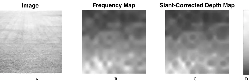
6.3 Natural images

The final two images are natural images, showing how the algorithm can handle the variety of textural properties generated by the variety of the natural world. Figure 11 is the uniform texture gradient of a lawn containing much fine detail.

The algorithm captures the primary near-to-far distance (light-to-dark gradient) represented by the depth structure of the lawn, although this is overlaid with some noisy structure that is less evident to the human eye.

A B C D

Figure 11. Simple natural texture gradient of a grassy field. Coding as in Figure 7.

Image Frequency Map Slant-Corrected Depth Map

Image

Frequency Map

Slant-Corrected Depth Map

Image Frequency Map Slant-Corrected Depth Map

Image

Frequency Map

Slant-Corrected Depth Map

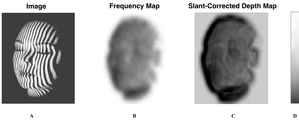
Figure 12 is a natural image of a face illuminated artificially by a linear graticule to define the facial contours, which would be essentially invisible in uniform illumination. This approach is used in some medical applications to bring out the depth structure of bodily images, which can be ill-defined even in stereoscopic view due to the sparsity of the contours over the

natural curved surface of the face and body. The algorithm does a respectable job of defining the overall curvature of the face and the hollows of the eyes and mouth, although the graticule density in this example is not sufficient to provide a high-resolution reconstruction.

A B C D

Figure 12. Natural image of a face illuminated by a contouring graticule. Coding as in Figure 7.

Finally, Figure 13 depicts a gloved hand with one striped texture is grasping a stockinged leg of another texture under a skirt of a third striped texture. It is noteworthy that the frequency algorithm captures the curvature of the leg and crinkles in the skirt while successfully delineating the three

different texture regions with darker outlines. This version of the algorithm does not parcellate the different texture into separate regions, but it is clear that it is tracking regions of similar texture through large gradient changes while strongly demarcating the boundaries between changing textures.

A B C D

Figure 13. Quasi-natural image of a textured hand grasping a textured leg. Coding as in Figure 7.

Image

Frequency Map

Slant-Corrected Depth Map

Image

Frequency Map

Slant-Corrected Depth Map

7 Discussion

As in the results shown above, this texture gradient based approach has succeeded in creating accurate depth maps for textured surfaces that correspond with the ground truth for many different artificial and natural images. This is proof of principle that the 2D peak Fourier frequency approach to 3D shape from texture has much to offer in terms of decoding object structure in both artificial and natural scene images. As stated earlier, most approaches in computer vision, utilize cues other than texture. Depth from stereo, depth from defocus, and depth from shading. are the main cues used to form depth maps. Even within textural approaches, most approaches are based on edge detection [7], which, although it does provide useful clues, cannot be used to understand a full map of depth within an image because it provides no information about the regions between the edges. The present texture gradient based approach is a valuable addition to the more popular approaches because it is derived from a single scene image, but it also has

its own requirements and assumptions. First and foremost, textural information must be well-defined, in that a high resolution natural image is required. This also means that, for non-textural images, such as the sky, depth cannot be extracted. The base depth is extracted using the perspective assumption that the frequency of a homogeneous texture increases with distance, which necessarily applies to natural images derived from a focal optical system.

This approach is different from most previous approaches utilizing texture because it provides the estimated textural map with less restrictive assumptions. Our approach can also be used easily to enhance various other forms of depth maps. The frequency map can and integrated with the base depth map from any other depth cue to enhance the overall depth map. As a result of this, various cues such as shading and stereopsis can be integrated to form more accurate depth maps, extending this approach to not only single images, but multiple images.

8 Applications

This 3D shape from texture computational method has powerful applications in the world of image understanding. As shown in Figures 11-13, this approach can be used in natural images, and can be a powerful extension and enhancement to a binocular disparity map.

Aside from applications in real life, this approach can be useful in approximating local depth. The ability to coarsely identify depth in anatomical structures such as faces, skulls, and bodies (see Figure 12-13) has medical applications, as depth can be achieved through one image without using complex and

complicated sensors. This method could also be used for virtual reality with 360° capture to create multiple views from sufficient number of cameras. In all the applications that would require more accurate depth maps, the texture gradient analysis can be used to improve the differential depth maps in regions of ambiguous correspondence matching in complex self-similar textures.

Acknowledgments: Thanks to the Smith-Kettlewell Eye Research Institute for a summer internship for AG.

9 References

[1] J.J. Gibson The Perception of the Visual World. Boston: Houghton Mifflin (1950).

[2] B. Potetz and T.S. Lee. "Scene statistics and 3D surface perception. "Computational Vision: From Surfaces to Objects. C.W. Tyler, Ed., Boca Raton, FL: Chapman & Hall, 1-25, (2010). [3] C.W. Tyler. “Cyclopean Vision”. In, Vision and Visual Disorders.

Vol. 9, Binocular Vision. Regan D. (Ed.), Macmillan: New York, 38-741 (1991).

[4] D. G. Lowe. "Object recognition from local scale-invariant features". Proceedings of the International Conference on Computer Vision 2:1150–1157 (1999).

[5] A. Blake and C. Marinos, “Shape from texture: estimation, isotropy and moments.” Artificial Intelligence, 45: 323-380 (1990).

[6] J. Malik and R. Rosenholtz “Computing local surface orientation and shape from texture for curved surfaces.” International Journal of Computer Vision 23(2): 149-168 (1997).

[7] D. Marr and E. Hildreth. "Theory of edge detection." Proceedings of the Royal Society of London B: Biological Sciences 207.1167:187-217 (1980).

[8] C.W. Tyler. "Theory of texture discrimination of based on higher-order perturbations in individual texture samples." Vision Research 44.18: 2179-2186 (2004).

[9] C.W. Tyler, ed. Computer Vision: from Surfaces to 3D Objects. CRC Press (2011).

[10] D. Scharstein, and R. Szeliski. "A taxonomy and evaluation of

dense two-frame stereo correspondence

algorithms." International Journal of Computer Vision 47.1-3: 7-42 (2002).

[11] D. Ziou, and F. Deschênes. "Depth from defocus estimation in spatial domain." Computer Vision and Image Understanding 81.2:143-165 (2001).