Understanding movement data quality

City, University of London Institutional Repository

Citation

:

10.1080/17489725.2016.1169322

This is the accepted version of the paper.

This version of the publication may differ from the final published

version.

Permanent repository link:

Link to published version

:

Copyright and reuse:

City Research Online aims to make research

outputs of City, University of London available to a wider audience.

Copyright and Moral Rights remain with the author(s) and/or copyright

holders. URLs from City Research Online may be freely distributed and

linked to.

Understanding Movement Data Quality

Gennady Andrienko, Natalia Andrienko, Georg Fuchs

* Fraunhofer Institute IAIS, Sankt Augustin, Germany and City University London, UK

Abstract

Understanding of data quality is essential for choosing suitable analysis methods and interpreting their results. Investigation of quality of movement data, due to their spatio-temporal nature, requires consideration from multiple perspectives at different scales. We review the key properties of movement data and, on their basis, create a typology of possible data quality problems and suggest approaches to identifying these types of problems.

Keywords: Movement data, data quality, visual analytics

1. Introduction: Position Recording

Analysis of movement data is of high relevance in various application domains of data science. As for

any analysis, appropriate data preparation, including investigation of the data quality, data cleaning, and

error correction, is essential. Data preparation is typically the most time-consuming step in the analysis

(Pyle 1999).

Movement data consist of records containing identifiers of moving entities (also called movers),

geographic and temporal references, and, possibly, other attributes, called thematic. A chronologically

ordered sequence of position records of the same mover (i.e., with the same mover identifier) is called a

trajectory of this mover. Thematic attributes may characterize the movement itself (e.g., the velocity and

direction) or the context in which the movement occurs (e.g., the air temperature). Such attributes can be

originally present in the data or derived from the records of the same trajectory, other trajectories, and

Evaluation and preparation of movement data requires particular diligence due to their inherent

complexity and the variation of properties related to the diversity of the existing methods of data

acquisition. Abstracting from the various specific technologies for collecting movement data, we

identify several major methods of position recording (Andrienko et al. 2008):

 Time-based: positions of movers are recorded at regularly spaced time moments.

 Change-based: a record is made when mover's position, speed, or movement direction differs from the previous one.

 Location-based: a record is made when a mover enters or comes close to a specific place, e.g. where a sensor is installed.

 Event-based: positions and times are recorded when certain events occur, in particular, when movers perform certain activities, such as cellphone calls or posting georeferenced contents to

social media.

 Combinations of these basic approaches. In particular, GPS tracking devices may combine time-based and change-time-based recording: the positions may be measured at regular time intervals but

recorded only when significant changes of position, speed, or direction occur.

In the following, we review the properties of movement data, potential quality problems, and the

consequent implications and constraints for analysis and modeling. In the long-term perspective, we aim

at defining general rules and procedures for assessing movement data quality. This paper makes first

steps towards this goal by systematically considering relevant properties of movement data (section 2)

and, based on that, identifying the expectable problems and errors (section 3), divided into three major

categories: missing data, accuracy errors, and precision errors. These categories are considered in more

detail in sections 4, 5, and 6, respectively. We conclude the paper by considering the role of data

2. Properties of Movement Data

In analyzing movement data, it is important to take into account their structure and properties

(Andrienko et al. 2013a). The first group of properties relates to the data structure:

 Mover set properties:

o number of movers: a single mover, a small number of movers, a large number of movers;

o population coverage: whether there are data about all movers of interest for a given

territory and time period or only for a sample of the movers;

o representativeness: whether the sample of movers is representative, i.e., has the same

distribution of properties as in the whole population, or biased towards individuals with

particular properties.

 Spatial properties:

o spatial resolution: what is the minimal change of position of an object that can be

reflected in the data?

o spatial precision: are the positions defined as points or as locations having spatial extents

(e.g. areas)? For example, the position of a mobile phone call is typically a cell in a

mobile phone network;

o position exactness: how exactly could the positions be determined? Thus, a movement

sensor may detect an object within its range but may not be able to determine the exact

coordinates of the object within its detection area. The object position may be specified

as a point, but, in fact, it is the position of the sensor and not the object’s true position;

o spatial coverage: are positions recorded everywhere or, if not, how are the locations

where positions are recorded distributed over the studied territory (in terms of the spatial

extent, uniformity, and density)?

 Temporal properties:

o temporal resolution: the lengths of the time intervals between the position measurements;

o temporal regularity: whether the length of the time intervals between the measurements is

constant or variable for selected movers and for the whole data set;

o temporal coverage: whether the measurements were made during the whole time span of

the data or in a sample of time units, or there were intentional or unintentional breaks in

the measurements;

o time cycles coverage: whether all positions of relevant time cycles (daily, weekly,

seasonal, etc.) are sufficiently represented in the data, or the data refer only to subsets of

positions (e.g., only work days or only daytime), or there is a bias towards some

positions.

The 2nd group relates to the data collection procedure:

 Data collection properties:

o position exactness: How exactly could the positions be determined? Thus, a movement

sensor may detect an object within its range but may not be able to determine the exact

coordinates of the object within its detection area. In this case, the position of the sensor

stands in for the object's true position;

o positioning accuracy, or how much error may be in the measurements;

o missing positions: in some circumstances, object positions cannot be determined, leading

o meanings of the position absence: whether absence of positions corresponds to stops, or

to conditions when measurements were impossible, or to device failure, or to private

information that has been removed.

These properties of movement data are strongly related to the data collection methods. Thus, only

time-based measurement produces temporally regular data. The temporal resolution may depend on the

capacities and/or settings of the measuring device. GPS tracking, which may be time-based or

change-based, typically yields very high spatial precision and quite high accuracy1 while the temporal and

spatial resolution depends on the device settings. The spatial coverage of GPS tracking is very high

(almost complete) in open areas. Location-based and event-based recordings usually produce temporally

irregular data with low temporal and spatial resolution and low spatial coverage. The spatial precision of

location-based recordings may be low (positions specified as areas) or high (positions specified as

points), but even in the latter case the position exactness is typically low. The spatial precision of

event-based recording may be high while the accuracy may vary (cf. positions of photos taken by a

GPS-enabled camera or phone with positions specified manually by the photographer).

Irrespectively of the collection method and device settings, there is also indispensable uncertainty in

movement data (and, more generally, any time-related data) caused by their discreteness. Since time is

continuous, the data cannot refer to every possible instant. For any two successive instants t1 and t2

referred to in the data there are moments in between for which there are no data. Therefore, one cannot

know definitely what happened between t1 and t2. Movement data with fine temporal and spatial

resolution give a possibility of interpolation, i.e., estimation of object positions between the measured

positions. In this way, the continuous path of the mover can be approximately reconstructed.

1 _{GPS: Error analysis for the Global Positioning System.}

Movement data that do not allow valid interpolation between subsequent positions are called episodic

(Andrienko et al. 2012). Episodic data are usually produced by location-based and event-based

collection methods but may also be produced by time-based methods when the position measurements

cannot be done sufficiently frequently, for example, due to the limited battery lives of the recording

devices. Thus, when tracking movements of wild animals, ecologists have to reduce the frequency of

measurements to be able to track the animals over longer time periods.

Whatever the measurement frequency is, there may be time gaps between recorded positions that are

longer than usual or expected according to the device settings, which means that some positions may be

missing. In data analysis, it is important to know the meaning of the position absence: whether it

corresponds to absence of movement, or to conditions when measurements were impossible (e.g., GPS

measurements in a tunnel), or to device failure, or to private information that has been intentionally

removed.

Another set of properties of movement data is related to the physics of the moving objects and the

character of their movement. These properties seriously affect the choice of the methods for data

pre-processing, transformation, visualization and analysis:

 Whether positions can be considered as two-dimensional, or the third dimension (altitude or depth) is essential.

 Whether the data represent constrained or free movement. When the movement is constrained, e.g., by a street network, there are better possibilities for detecting and correcting positioning

errors and for reducing position uncertainties.

 Whether movements may contain abrupt changes of the spatial position in very short time. For example, a pertinent property of eye movement is the presence of instantaneous jumps (saccades)

end positions of a saccade are not meaningful: it cannot be assumed that there exists a straight or

curved line between two fixation positions such that the eye focus travels along it attending all

intermediate points. This prohibits the use of any method involving interpolation between

positions.

3. Typology of movement data quality problems

There are three major categories of problems that may exist in any kind of data: missing data, accuracy

problems, and precision deficiency. For movement data, these general categories may be specialized in

terms of the data components: identities of movers, spatial positions, time references, and thematic

attributes.

When any of the main components (i.e., mover identifier, spatial position, or time reference) is missing

in a data record, this record cannot be used in constructing a trajectory; hence, the absence of one of the

main components is equivalent to the absence of the entire position record. Missing values of thematic

attributes do not have so dramatic impact. Problems arise only in particular analyses requiring these

attributes to be involved. In the following, we shall consider only the cases of missing records.

Accuracy problems (i.e., wrong values, or errors) may occur to any of the movement data components.

Precision deficiency problems may occur to spatial positions, time references, and thematic attributes.

Imprecise mover identifiers are equivalent to wrong identifiers: in both cases, position records cannot be

correctly grouped into trajectories of movers.

Hence, for movement data, the specific types of possible problems are: missing position records

(abbreviated as M), accuracy problems affecting mover identifiers, spatial positions, time references,

and thematic attributes (AMv, AS, AT, and AAt, respectively), and precision deficiency for spatial

The scope of problem spread in a dataset can be evaluated from different perspectives. For a single

trajectory, problems may occur in some position records, in subsequences of records (segments of the

trajectory), or in the whole trajectory. Adapting Bertin (1983) terminology, we call such problems

elementary, intermediate, and overall, respectively, and abbreviate as TrE, TrI, and TrO.

Furthermore, the spread of a problem may be characterized with regard to the value domains of the three

main components, i.e., the set of movers Mv, space (set of locations) S, and time (set of moments) T.

Problems may refer to individual movers, locations, and moments (elementary level MvE, SE, and TE),

to groups of movers, areas in space, or periods in time (intermediate level MvI, SI, and TI), or to the

entire set of movers, whole territory, and whole time span of the data (overall level MvO, SO, and TO).

Assuming one-to-one correspondence between the movers and trajectories, the problem spread over the

mover set means the spread over the set of trajectories.

In evaluating the quality of a given dataset, an analyst needs to check, for each problem type, whether it

exists in the data and, if so, determine the scope of the problem spread in the trajectories and over the

value domains of the three main components.

In the following sections, we shall consider in more detail the problems of missing position records,

inaccuracy (errors), and insufficient precision. We shall discuss the possible scopes of the spread of such

problems in relation to their possible reasons, propose approaches to problem detection and scope

evaluation, and give prominent examples of problems encountered in various real datasets.

4. Missing Position Records

The main focus of this section is consideration of the possible spread of the missing data problem over

the space and time. In this relation, we shall also touch upon the problem spread within trajectories and

4.1. Spatial spread

Missing position records within trajectories are signified by spatio-temporal gaps between available

records, i.e., where the spatial and/or temporal distances between consecutive records are larger than

usual or expected. This class of problems may be represented as M: TrE/I, where TrE/I means that

occasional positions in a trajectory (TrE) or trajectory segments (TrI) may be missing. Trajectory

segments with large spatial and/or temporal distances between consecutive positions can be extracted

from a set of trajectories by means of threshold-based filtering. To analyze the spatial spread and find

the possible reason for the problem, the extracted segments are visualized on a map, which will show

either spatial scattering or concentration of the gaps.

When the extracted gaps are scattered over space (which means the elementary level of the spatial

spread M:SE), a possible reason may be occasional failures of measuring devices. When the gaps are

concentrated in particular parts of space (areas or segments of a transportation network), i.e., the level of

the spatial spread is intermediate (M:SI), a possible reason may be impossibility of position measuring

in these parts of space, e.g., GPS positioning is impossible in covered spaces. Another possible reason

may be a particular way of data filtering. For example, a subset of data may be extracted from a larger

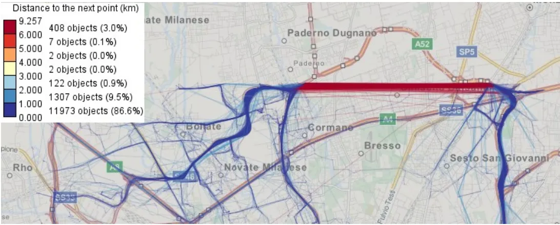
data set by setting a bounding rectangle covering some area of interest. Figure 1 demonstrates a case

when a data provider just removed all positions that lied beyond the bounding rectangle. This lead to

specific cases of data absence when cars temporarily moved out of the area enclosed by the rectangle

and returned back after few minutes. When trajectories are represented on a map by lines, the trajectory

lines of these cars have unrealistic straight segments connecting the last position before leaving the

rectangular area and the first position after returning back. Trajectory segments corresponding to

cutting-caused gaps are spatially concentrated at the edges of the studied area. In Figure 1, only the

affected trajectories are shown; the segments of the trajectories are colored according to the spatial

Figure 1. Segments are missing in many trajectories due to cutting of the data by a bounding rectangle.

In case of location-based recording, measuring devices are only present in particular locations; therefore,

spatio-temporal gaps between records occur in all other parts of the territory. The degree of the spatial

spread can be characterized as overall (SO). The same applies to event-based recording: gaps, which

occur due to the absence of events during long time intervals, can be distributed over the whole space. In

episodic movement data resulting from such methods of measurement, spatio-temporal gaps are usual

and pertinent to whole trajectories of all movers, which can be represented as M: TrOMvOSOTO. Only in some cases, intermediate positions can be estimated using additional data sets such as street

network and speed limits.

In time-based recording, the spatial distances between position records depends on the movement speed.

If the speed is high, spatial (but not spatio-temporal) gaps may emerge. This problem refers to parts of

trajectories where the speed is high and to the intermediate or overall level with regard to the mover set,

space, and time (M: TrE/IMvI/OSI/OTI/O), depending on the movers’ capacities to develop high speed and the possibilities of fast movement in different parts of space and at different times. Often,

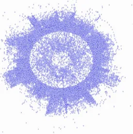
In change-based recording, parameter settings may cause systematic omissions of position records. For

example, a GPS tracker may skip mover’s positions during straight-line movement with constant speed

when the distance to the last recorded position is below a certain distance threshold. Such data property

can be identified by plotting trajectory points according to the changes of their coordinates (X,Y) with

respect to the previous points. An example is shown in Fig. 2. The circular area of low point density in

the center of the graph has the radius of 20 meters, which reveals the value of the filter threshold.

Positions missed due to such straight-line filtering can be quite easily restored by linear interpolation.

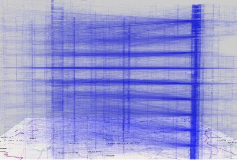
The scope of the problem may be represented as M: TrE/TrIMvOSITO, where SI means that problems occur in particular parts of space where straight line movement is possible.

Figure 2. A plot of coordinate changes (X,Y) in respect to the previous trajectory points reveals an

effect of filtering.

4.2. Temporal spread

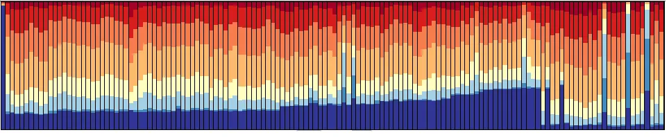
such as a temporal histogram demonstrated in Figure 3. The data used for this example are mobile phone

activation records, where the positions are specified by references to antennas of a telecommunication

network. The data have been aggregated by the antennas and daily intervals. Each bar of the histogram

corresponds to one day; the bars are chronologically ordered. The whole height of each bar corresponds

to the whole set of antennas, and the height of a dark blue segment is proportional to the number of

antennas for which there are no phone activation records for the day corresponding to the bar. The other

segment colors correspond to different numbers of records per antenna and day; the shades of blue

represent low numbers and the shades of red high numbers.

An absence of records referring to some antenna during a time interval corresponds to spatio-temporal

gaps (missing segments) in trajectories of movers that might have used or attempted to use their phones

within the antenna range during that time interval (M: TrI). The histogram in Fig. 3 shows that every day

records were missing for some antennas; moreover, the number of antennas with missing data was

monotonously increasing over time, except for the last two weeks. Besides, there were days when the

numbers of antennas with no or few records (shades of blue) were especially high. The level of the

temporal spread of the missing data problem in this dataset can be characterized as overall (M: TO) and

the level of the spatial spread as intermediate (M: SI), since subsets of the set of locations (i.e., antenna

cells) are affected. The problem, evidently, affects large groups of movers (M: MvI). The whole formula

is M: TrIMvISITO.

Additionally to the distribution of a problem (missing data or any other type) over the time span of the

data considered as a linear sequence of time moments, it is appropriate to investigate how the problem is

distributed with regard to relevant time cycles, such as daily, weekly, and yearly. Thus, gaps in data may

occur or be especially frequent in particular times of a day and/or days of a week. To detect such

temporal patterns of problem spread, histograms as in Fig. 3 can be built for relevant time cycles.

Figure 4. A map with mosaic diagrams represents the same data as in Figure 3. The diagrams placed at the antenna positions show the daily record numbers for the antennas. The dark blue pixels represent days with no records.

4.3. Spatio-temporal spread

happen that problem occurred at different times in different parts of space. To check whether this is the

case, the analyst can use a map with diagrams showing the problem occurrences over time at different

locations or in different areas. An example is demonstrated in Fig. 4, where the map represents the same

data as in Fig. 3. The mosaic diagrams represent counts of recorded mobile phone activations at different

antennas by days. Each day is represented by a colored pixel. The pixels within a diagram are arranged

in rows with columns correspond to days of the week (Monday to Sunday), for a total of 20 rows

matching the 20-week time span of the data. Dark blue pixels correspond to zero counts, i.e., absence of

phone activation records for the given day. It can be seen that on the south the data are available only for

the last two weeks. On the west, there are several consecutive weeks with missing data. Time gaps are

also noticeable for some antennas on the northeast. In the center of the territory, there is an antenna

(highlighted) with no records on the weekends.

5. Accuracy problems

5.1. Mover identity errors

Trajectories of movers are constructed by uniting consecutive positions of each mover. The positions of

different movers are distinguished based on the identifiers contained in the position records. Hence, each

mover needs to have a unique identifier. However, this condition may not always hold. Two kinds of

mover identity errors are possible: (1) the use of the same identifier for two or more different movers

and (2) the use of different identifiers for the same mover. If two distinct movers have the same

identifier, their positions will be mixed in one trajectory. This is especially well noticeable when the

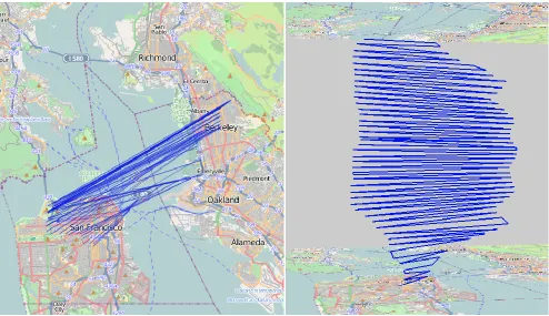
movers move simultaneously. An example is demonstrated in Figure 5. The cases of occasionally

duplicated mover identifiers can be recognized from unrealistic values of derived speeds and/or

unusually long spatial distances between consecutive positions. Identification of such errors can be

of different movers with the same identifier are separated in time, the duplication of the identifier may

be undetectable. Cases of occasional duplication of mover identifiers may be represented as AMv: MvE.

Figure 5. Positions of two distinct movers with the same identifier have been mixed in one trajectory, which therefore has a zigzag shape.

Identifiers given to movers are not necessarily kept constant throughout the whole time of data

collection. For preserving personal privacy or other reasons (e.g., hiding sensitive repeated patterns in

business-related movement data), movers may be assigned new identifiers at certain time intervals, e.g.,

every day or every two weeks. The previous identifiers may be reused for different movers. Moreover,

in different time intervals, the data may correspond to different samples of the population. Hence, in

such cases, both problems arise: same identifiers may be used for different movers and different

identifiers for same movers. The problems affect the whole set of movers (AMv: MvO). Such problems

identifiers. Assignments of previously used identifiers to new movers will be manifested by unusually

long jumps in space occurring in many trajectories at regular time intervals. An example is shown in a

space-time cube in Figure 6, where a sample of trajectories is drawn with 1% opacity. Bunches of long

near-horizontal lines occur every two weeks. It is very unlikely that they reflect real movements; most

probably, they reflect re-assignments of mover identifiers. A case when old identifiers are not reused but

new unique identifiers are assigned to movers can be recognized from the statistics of trajectory

durations. The maximal duration will not exceed the length of the time interval between the changes of

the identifiers.

5.2. Spatial errors

Spatial accuracy problems are often caused by malfunctioning positioning devices or difficult conditions

for measurements. Thus, GPS positioners need to establish connections with several satellites, which

takes time. During this time, the recorded positions, if any, may be inaccurate. If such a device is turned

on only when a trip begins, the departure position of the trip and the trajectory segment representing the

initial part of the trip may be missing or wrong (Figure 7). This case may be represented by the formula

MAS: TrI. The spread of the problem over the set of movers, space, and time depends on how many movers and for how long were tracked by such devices and whether the data reflect repeated trips of the

movers.

Figure 8 demonstrates another example, where the spatial positions in a whole trajectory, shown in red,

are erroneous (AS: TrO), combining noise (jitter) with a systematic shift to the northwest with regard to

the true positions. The shift was detected by comparing the spatial footprints of different trajectories

available in the dataset. In this dataset, only one trajectory was erroneous (AS: TrOMvE).

Jitter may also occur in parts of trajectories corresponding to stops or movement with low speed. In such

conditions, GPS readings may be inaccurate. Very often stops appear in data as fake jittered movement

Figure 7. The starting parts of many trips are missing. The yellow dot symbols show the recorded positions of the trip starts.

Figure 9. Stop positions appearing as jittered movement.

5.3. Temporal errors

Generally, time references in movement data are more accurate when spatial positions. However, we are

aware of three cases when temporal errors may have significant spread. Thus, trajectories built from

metadata of flickr photos of tourists often have shifted time references because users forget to change

the time zone in their cameras or mobile devices. The second case is one-hour shift occurring if the

daylight saving time is not adjusted properly. Third, often photo capture time is replaced by upload time.

While the second and third cases are quite easy to detect by inspecting temporal histograms of position

counts, the first case requires more sophisticated processing.

5.4. Attribute errors

Obviously, missing data and errors in the main components of movement data cause errors in thematic

movement are calculated from pairs of sequential positions. Both first derivatives (e.g. speed) and higher

order derivatives (e.g. acceleration) are affected by spatio-temporal gaps and incorrect identities, spatial,

and temporal references. Furthermore, aggregated attributes for whole trajectories, such as total length

or average speed, are also affected.

Generally, derived thematic attributes depend on the sampling rate in the data, i.e., temporal frequency

of recorded positions (Laube and Purves 2011). Thus, due to the triangle inequality, a decrease of the

sampling rate causes a decrease of the computed distance between position records and, further on, a

decrease of the speed.

6. Precision deficiency

While spatial positions in the real world are continuous, their computer representation is discrete.

Depending on the precision of position representation, different real spatial positions may be represented

in data as the same position. Moreover, due to rounding, all position records may form spatial clusters of

frequently recorded positions (PS: TrOMvOSO). These are false patterns that do not correspond to real-world phenomena.

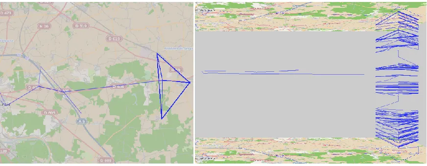
Specific cases of spatial precision errors occur in trajectories constructed from mobile phone use data.

When a phone is in the range of two or more neighboring antennas, it can switch from one antenna to

another without any movement of the phone carrier. As a result, the trajectory may contain jumps

between positions of different antennas that do not represent real movement of the user. In Figure 10, an

example of such trajectory is shown on a map (left) and in a space-time cube (right). Some of the jumps

Figure 10. A trajectory of a mobile phone user contains segments of false movement caused by switching the phone connection between neighboring antennas.

Loss of precision in time references may lead to appearance of multiple position records of the same

mover referring to the same time. It may be impossible to put these records in the right order for

reconstructing the corresponding trajectory segment. Therefore, the segment has to be replaced by one

representative position, e.g., the most central position or the average of all positions.

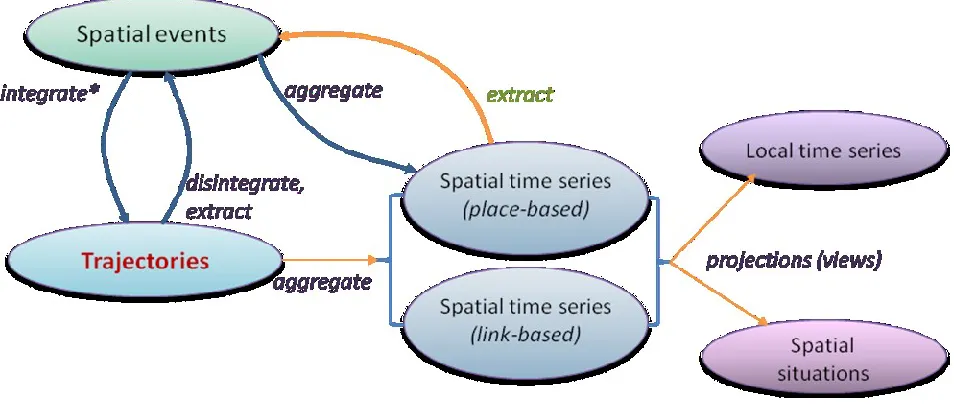
7. Conclusion

Different representations of the same data may be more suitable for answering specific analysis

questions depending on what data aspect(s) (what, where, when) (Peuquet 2002) are in focus. For

movement data, there are three principal representations (Andrienko et al. 2013a) (Fig. 11). Conversions

between these representations may be useful not only for supporting different types of analysis tasks but

also for detecting different kinds of problems. One example is shown in Fig. 4, where movement data

are viewed as spatial time series. After transforming data to another representation, it is advisable to

search for patterns such as spatial or spatio-temporal clusters, extreme values, etc. Any kind of

unexpected irregularity or regularity, either temporal or spatial, may correspond to problems in original

Figure 11. The principal transformations applicable to movement data, depending on the task/analysis goal.

Data preparation is typically the most time-consuming step in the analysis process, and thus proper tool

support for this phase is highly important. This holds especially true for movement data with its inherent

complexities. In this paper, we have shown visualizations that reveal the existence of different problems

and the degrees of their spread. We have also mentioned some computational operations that help in

problem detection. Since data quality analysis requires human judgement, it cannot be done fully

automatically; however, the work of a human analyst may be supported by an “intelligent checklist” tool

reminding what kinds of problems need to be investigated, making appropriate computations and data

transformations, and generating informative visualizations.

References

Andrienko G, Andrienko N, Bak P, Keim D, Wrobel S (2013a) Visual analytics of movement. Springer, Berlin

Andrienko N, Andrienko G, Pelekis N, Spaccapietra S (2008) Basic concepts of movement data. In Mobility, Data Mining and Privacy – Geographic Knowledge Discovery, Giannotti F, Pedreschi D, (Eds.). Springer Verlag, Heidelberg, 2008, ch. 1, 15–38.

Andrienko N, Andrienko G, Stange H, Liebig T, Hecker D. (2012) Visual Analytics for Understanding Spatial Situations from Episodic Movement Data. Künstl Intell 26(3):241–251.

Bertin J (1983) Semiology of Graphics. Diagrams, Networks, Maps. University of Wisconsin Press, Madison. Translated from Bertin, J.: Sémiologie graphique, Gauthier-Villars, Paris, 1967.

Dodge S, Weibel R, Forootan E (2009) Revealing the physics of movement: Comparing the similarity of movement characteristics of different types of moving objects. Computers, Environment and Urban Systems 33(6):419–434.

Dodge S, Weibel R, Lautenschütz A-K (2008) Towards a taxonomy of movement patterns. Information Visualization 7(3-4):240–252.

Laube P, Purves RS (2011) How fast is a cow? Cross-Scale Analysis of Movement Data. Transactions in GIS 15(3): 401-418.