Corresponding author: Erkan Oterkus, University of Strathclyde, PeriDynamics Research Centre, Glasgow G4 0LZ, United Kingdom, E-mail: [email protected]
A Kirchhoff Plate Formulation in a State-Based Peridynamic Framework
Zhenghao Yang1, Bozo Vazic1, Cagan Diyaroglu2, Erkan Oterkus1 and Selda Oterkus1
1PeriDynamics Research Centre University of Strathclyde, Glasgow, UK
2Aerospace and Mechanical Engineering Department University of Arizona, Tucson, USA
Abstract
In recent years, there has been rapid progress on peridynamics. It has been applied to many different material systems, used for coupled field analysis and it is suitable for multi-scale analysis. This study mainly focuses on peridynamic analysis for plate-type structures. For this purpose, a new peridynamic Kirchhoff plate is developed. The new formulation is computationally efficient by having only one degree of freedom for each material point. Moreover, it is based on state-based peridynamic formulation which doesn’t impose any limitation on material constants. After presenting how to impose simply supported and clamped boundary conditions in this new formulation, several numerical studies are considered to demonstrate the accuracy and capability of the proposed formulation.
1. Introduction
Peridynamic (PD) theory was introduced by Silling (2000) as an alternative formulation to Classical Continuum Mechanics (CCM). Instead of expressing equations of motion in partial differential equation form as in CCM, peridynamic equations of motion are expressed in integro-differential equation form. Moreover, peridynamic equations do not contain any spatial derivatives which offer certain advantages especially for the solution of problems including displacement discontinuities due to the existence of cracks. Besides, in peridynamics, the state of a material point is influenced by material points which are located at a finite distance within a domain of influence called as horizon. This feature positions peridynamics within non-local continuum mechanics formulations. As highlighted in dell’Isola et al. (2015), the origins of peridynamics go back to Piola. Since its introduction, there has been rapid progress on peridynamics. The PD formulation has been applied to many different material systems including linear elastic materials, metals and composite materials (Oterkus and Madenci, 2012). The PD theory is not limited to macroscopic analysis which allows researchers to use it for analyzing problems at mesoscale (De Meo et al., 2016) and nano-scale (Ebrahimi et. al., 2015). Moreover, it is currently possible to perform multi-physics analysis in a single peridynamic framework by coupling mechanical field to thermal field (Oterkus et. al., 2014a), moisture diffusion (Oterkus et. al., 2014b), electric current (Gerstle et. al. 2008), porous flow (Oterkus et al., 2017), etc. PD theory has also been effectively used for impact analysis (Amani et al., 2016). An in-depth review of PD research is given in Madenci and Oterkus (2014) and Javili et al. (2018).
formulation suitable for modelling thin plates using rotational springs between peridynamic bonds. Diyaroglu et al. (2015) developed a bond-based PD Mindlin plate formulation which takes into account the effect of shear deformation and is suitable for the analysis of thick plates.
In this study, a new PD Kirchhoff plate formulation is presented. This new formulation has certain advantages. First of all, each material point has only one degree of freedom, i.e. transverse deflection, as opposed to three-degree of freedom used in Mindlin plate formulation. This yields significant computational time and memory reduction in computations. Moreover, the formulation is based on PD state-based concept. Therefore, it doesn’t impose any limitation on material constants. The paper starts with a derivation of the equation of motion for the new PD Kirchhoff plate formulation. It then presents how to apply simply supported and clamped boundary conditions in the current formulation. Finally, several numerical cases are demonstrated to show the accuracy and capability of the proposed formulation.
2. Kinematics of Kirchhoff plate
Unlike the local continuum theory, in PD theory, each state of a material point is not only influenced by the material points located in its immediate vicinity but also influenced by material points which are located within a region of finite radius named as “horizon”, H. Therefore, the general PD equations of motion for material point x k can be expressed in summation form as (Madenci and Oterkus, 2014)
2 ( ) 2
1
j
N k
k k j j k
j
V t
u
f b (1)
where the summation takes over the family member material points of k and Nk indicates the total number of family members, , u, t, V and b represent the density, displacement, time, material point volume and the body load vector, respectively. The interaction force vector,
k j
f , between material points k and j has a unit of “force per unit volume squared” defined as (Madenci and Oterkus, 2014)
k j k j j k
f t t (2)
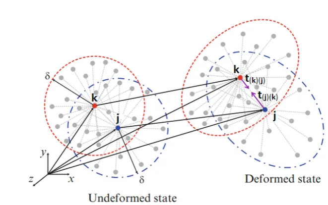
As shown in Fig. (1), the PD force density vector t k j represents the force acting on the main material point k by its family member material point j, and, on the contrary, t j k represents the force acting on material point j by its family member material point, k. They are also related to strain energy density function, W k , as (Madenci and Oterkus, 2014)
1 k
k j
j j k
W
V
t
u u (3a)
1 j
j k
k k j
W
V
t
[image:3.595.116.447.113.320.2]u u (3b)
Figure 1. Peridynamic interaction force vectors.
Kirchhoff plate theory is based on the assumption that “normals to the mid-surface of the undeformed plate remain straight and normal to the mid-surface, and unstretched in length, during deformation.” To derive PD force densities of Kirchhoff plate theory (Fig. 2), the strain energy densities of material points k and j are expressed as (Leissa and Qatu, 2011)
2 2
1
2 1 2
k k k k k
x y xy x y
k
D W
h
(4a)
and
2 2
1
2 1 2
j j j j j
x y xy x y
j
D W
h
(4b)
where 3 12 1
2
DEh is the flexural rigidity, is the Poisson’s ratio and h is the thickness of the plate. The linearized curvatures and twist of the plate mid-surface, x, y and xy, are expressed as
2 , ( , )
2 k j k j
x
w x
,
2 , ( , )
2 k j k j
y
w y
and
2 , ( , )k j k j xy
w x y
(5)
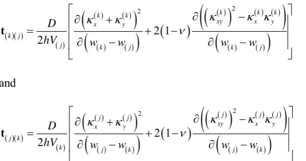
2 2 2 1 2k k k
k k
xy x y
x y
k j
j k j k j
D
hV w w w w
t (6a)
and
2 2 2 1 2j j j
j j
xy x y
x y
j k
k j k j k
D
hV w w w w
t (6b)
The PD form of linearized curvatures and twist can be derived for the material point xfrom Taylor series expansion by ignoring the higher-order terms,
3x
as
2 2 2 2 2 2 2 3 1 1 2 2x y x y
x y
w w w w
w w
x y x y
w x x y
x x x x
x ξ x
x (7)
where x and y are the projections of reference length x j x k between material points k and j along x- and y- axes, respectively, and they are defined as
cos
x
(8a)
and
sin
y
(8b)
[image:4.595.73.382.71.233.2]Note that represents the angle between the peridynamic interaction and x-axis as shown in Fig. 2. Substituting Eq. (8) into Eq. (7) and performing some algebraic manipulations result in
2
2 2 2
2 2
2 2
cos sin
1 1
cos sin cos sin
2 2
w w w w
x y
w w w
x y x y
x x x x
x x x (9)
As explained in Appendix A, if each term in Eq. (9) is multiplied with trigonometric functions of gi
while integrating over the circular horizon of the differentiations in Eq. (9) can be expressed in terms of integrations as
2 2 2
2 2 2 2
0 0
4
d d
w w w w
x y
x x x x
2 2
2 2
0 0 4
2 cos sin d d
w w w
x y
x x x
(10b)
2 2 2
2 2 2 2
0 0 0 0
2
d d 2 cos 2 d d
w w w w w
x
x x x x x
(10c)
2 2 2
2 2 2 2
0 0 0 0
2
d d 2 cos 2 d d
w w w w w
y
x x x x x
(10d)
Utilizing Eqs. (10a-d) for material points k and j and discretizing the integral equations, the curvatures and twist can be defined as
2 2
1 4 ik k
k k k N k i k k
x y i
i i k
w w V h
(11a) 2 2 1 4 2cos sin k k i
k k k
k k
N
k i k
xy i k i k i
i i k
w w V h
(11b)
2 2 2
1 1
2
2 cos 2
k k k k
i i
k k k
k k k k
N N
k k
i i
k
x i i k i
i i k i i k
w w w w
V V h
(11c) 2 2 2
1 1
2
2 cos 2
k k k k
i i
k k k
k k k k
N N
k k
i i
k
y i i k i
i i k i i k
w w w w
V V h
(11d)and they are for material point j
2 2
1 4 ij j
j j j N j i j j
x y i
i i j
w w V h
(12a) 2 2 1 4 2cos sin j j i
j j j
j j
N
j i j
xy i j i j i
i i j
w w V h
(12b)
2 2 2
1 1
2
2 cos 2
j j j j
i i
j j j
j j j j
N N
j j
i i
j
x i i j i
i i j i i j
w w w w
2 2 2
1 1
2
2 cos 2
j j j j
i i
j j j
j j j j
N N
j j
i i
j
y i i j i
i i j i i j
w w w w
V V h
(12d)where the summation indices k
i and ij represent the material points inside the horizon of the main material point k and its family member point j, respectively. Substituting Eqs. (11) and (12) into Eqs. (6a,b), and performing some algebraic manipulations, the PD force densities can be expressed in terms of displacements, w as
2 22 2 2
1
2 2 1
2 1 8cos 5
k k i k k k k N k i
k j i k j k i
i
j k i k
w w
D
V
h h
t (13a)
and
2 22 2 2
1
2 2 1
2 1 8cos 5
j j i j j j j N j i
j k i j j k i
i
j k i j
w w
D
V
h h
t (13b)
Substituting force density vectors t k j and t j k (Eq. 13) into interaction force vector, f k j (Eq. 2), the PD equation of motion (EOM) of Kirchhoff plate theory can be derived from Eq. (1) as
2 ( ) 2 2 2 1 2 4 3 21
2 2
1
2 1 8cos 5
8 1
2 1 8cos 5
k k i k k k k j j j i j j j j k k N k i j k
i k i
N i i k
k N
j j k i j
j k
i j i
i i j
Figure 2. PD interactions in Kirchhoff plate theory. 3. Boundary conditions
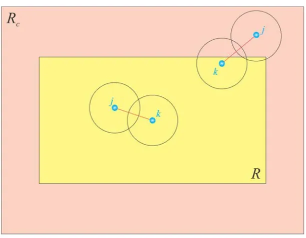
[image:7.595.145.451.264.501.2]The prerequisite of the derivation process of PD EOM is that the material points’ influence domain must be completely embedded in a material domain. For this reason, the PD EOM derived in Eq. (14) is valid only if the main material point, k and its family member, j have intact horizons which are fully embedded in an actual material domain, R, as shown in Fig. 3. However, near boundary points, k and j, can have incomplete influence domains. Therefore, the supplemental equations valid for the fictitious boundary layer, Rc, outside the boundary of the actual material domain, are necessary as explained in Madenci and Oterkus (2014). The width of this layer can be chosen as the double size of the horizon. The possible types of boundary conditions and their corrections are explained below for Kirchhoff plate theory from PD point of view.
Figure 3. The truncated horizons of k and j and the introduction of fictitious boundary layer
3.1 The clamped boundary condition
To implement clamped boundary condition (Fig. 4), a fictitious boundary layer is created outside the actual material domain. The horizon size can be chosen as 3 x in which the
discretization size is x. This horizon size is sufficient enough to represent macro-scale
displacements in plate problems (Diyaroglu et al, 2014). Hence, the width of the fictitious
region is chosen as 2 .
The clamped boundary condition for the vertical edges along the y-axis is obtained by imposing
zero displacements and zero rotation for the material points adjacent to the clamped end as
0 0w x and w x
0 0x
in which x0 is on the boundary line. Therefore, as shown in Fig. 4, the displacements of the material points close to the boundary line can be assumed as zero:
k 1 k 1 0 for 1, 2,...
w w k n (16)
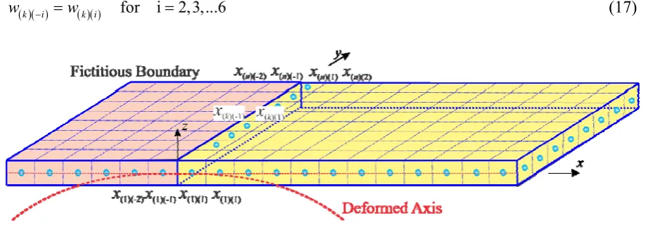
where the first subscript represents the number of rows along the y-direction and the second subscript is for the number of columns along the x-direction. The displacement field of material points near the boundary region are necessarily imposed to be symmetric to the clamped boundary as
k i k i for i 2,3,...6
[image:8.595.68.529.224.384.2]w w (17)
Figure 4. Clamped boundary condition.
Similarly, the horizontal direction edges parallel to the x-axis has constraint conditions of
0 0w y and w y
0 0 x
(18)
in which y0 is on the horizontal boundary line. The corresponding PD boundary conditions can be obtained as in Eqs. (16) and (17).
3.2. The simply supported boundary condition
To implement simply supported boundary condition, the fictitious boundary layer is again chosen to be equal to 2. The vertical direction boundaries (along the y-axis) are imposed to have zero displacements and curvatures as
0 0w x and
20
2 0
w x x
(19)
In the discretized form of PD formulation, these conditions can be achieved by enforcing anti-symmetrical displacement fields to the material points in the fictitious region as opposed to the actual displacement fields as shown in Fig. 5. Thus, it is defined as
k i k i for i 1, 2,...6 and 1, 2,...
Figure 5. Simply supported boundary condition. Similarly, the horizontal direction edges have the constraints of
0 0w y and
20
2 0
w y y
(21)
and in discretized form these conditions take a similar form as in Eq. (20).
4. Numerical Validation
To verify the validity of new PD formulation for a Kirchhoff plate, the PD solutions are compared with the corresponding finite element (FE) analysis results.
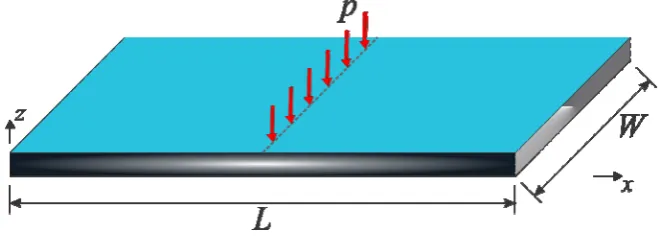
4.1. Clamped Plate
A clamped plate with a length and width of LW 1 m and a thickness of h0.01 m is considered as shown in Fig. 6. The Young’s modulus and Poisson’s ratio of the plate are
200 GPa
E and 0.3, respectively. The model is discretized into one single row of material points along with the thickness and the distance between material points is
0.01 m
x
. A fictitious region is introduced outside the edges as the external boundaries with a width of 2. The plate is subjected to a distributed transverse load of p100 N/m through the y-center line. The line load is converted to a body load of
5 10 N/m5 32 /
pW b
W x V
[image:9.595.129.462.567.685.2]and it is distributed to two columns of material volumes through the center line as shown in Fig. 7.
Figure 7. The PD discretization of a clamped plate.
[image:10.595.73.507.229.411.2](a) (b)
Figure 8. The comparison of the vertical displacement components of (a) FE and (b) PD results (unit: m).
(a) (b)
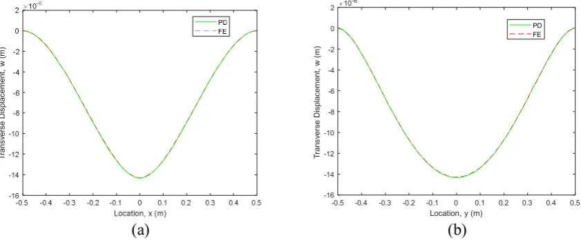
Figure 9. The comparison of the vertical displacements along a) x- and b) y- central axes
The FE model of the plate is created by using SHELL181 element in ANSYS. The PD and FE transverse displacement contours are compared in Fig. 8. They yield similar displacement variations. The maximum difference between PD and FE results is less than 0.5%. Moreover,
the vertical displacement components along central x- and y- axes are compared in Fig. 9. These
Tr
ans
ve
rs
e
Dis
plac
em
ent
,
w
(
m
)
-0.5 -0.4 -0.3 -0.2 -0.1 0 0.1 0.2 0.3 0.4 0.5
Location, y (m)
-16 -14 -12 -10 -8 -6 -4 -2 0 2
Tr
an
sv
er
se
D
is
pl
ac
em
en
t, w
(
m
)
10-6
[image:10.595.85.506.473.647.2]results verify the accurateness of the current PD formulation for a Kirchhoff plate theory under clamped boundary conditions.
4.2. Simply Supported Plate
A simply supported plate (Fig. 10) has the same geometrical and material properties as of the clamped plate case. Again, it is discretized with a single row of material points along the
thickness direction and the discretization size is x 0.01 m. A fictitious region is created
outside the region of boundaries and its width is equal to two times the size of the horizon, .
The plate is subjected to a distributed transverse line load of p100 N/m through the y-central
line. It is imposed to two columns of material points with a body load of 5 10 N/m5 3
[image:11.595.121.465.248.379.2]b as in
[image:11.595.77.498.439.621.2]Fig. 7.
Figure 10. The geometry of a simply supported Kirchhoff plate.
(a) (b)
[image:12.595.85.506.75.253.2]
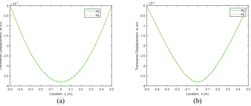
(a) (b)
Figure 12. The comparison of vertical displacements along a) x- and b) y- central axes. The transverse displacement components of FE and PD theory show very close variations as shown in Fig. 11. The maximum difference between PD and FE results is less than 0.5%. Furthermore, the displacement variations along central x- and y- axes are on top of each other for FE and PD results as shown in Fig. 12. This is to confirm the current PD formulation of Kirchhoff plate theory under simply supported boundary conditions.
5. Final remarks
This study presents a new state-based peridynamic formulation for Kirchhoff plate theory. The constitutive equation is obtained by utilizing the strain energy density of a material point in the form of curvatures and twist. Taylor series expansion up to the order of two is utilized to obtain PD form of strain energy density function. Due to the nonlocal characteristic of peridynamic theory, the boundary condition implementation needs extra care. Thus, implementation of two different type boundary conditions, clamped and simply supported, in the current formulation is presented. Two different numerical cases incorporating such boundary conditions are considered and very good agreement is observed between peridynamic and finite element analysis results.
References
Aguiar AR. On the determination of a peridynamic constant in a linear constitutive model. Journal of Elasticity 2016; 122(1): 27-39.
Amani J, Oterkus E, Areias P, Zi G, Nguyen-Thoi T and Rabczuk T. A non-ordinary state-based peridynamics formulation for thermoplastic fracture. International Journal of Impact Engineering 2016; 87: 83-94.
dell’Isola F, Andreaus U and Placidi L. At the origins and in the vanguard of peridynamics, non-local and higher-gradient continuum mechanics: An underestimated and still topical contribution of Gabrio Piola. Mathematics and Mechanics of Solids 2015; 20(8): 887-928.
De Meo D, Zhu N and Oterkus E. Peridynamic modeling of granular fracture in polycrystalline materials. Journal of Engineering Materials and Technology 2016; 138(4): p.041008.
Tr
an
sv
er
se
D
is
pl
ac
em
en
t, w
(
m
)
Tr
an
sv
er
se
D
is
pl
ac
em
en
t, w
(
m
Diyaroglu C, Oterkus E, Oterkus S and Madenci E. Peridynamics for bending of beams and plates with transverse shear deformation. International Journal of Solids and Structures 2015; 69-70: 152-168.
Ebrahimi S, Steigmann D and Komvopoulos K. Peridynamics analysis of the nanoscale friction and wear properties of amorphous carbon thin films. Journal of Mechanics of Materials and Structures 2015; 10(5): 559-572.
Gerstle W, Silling S, Read D, Tewary V and Lehoucq R. Peridynamic simulation of electromigration. Comput Mater Continua 2008; 8(2): 75-92.
Javili A, Morasata R, Oterkus E and Oterkus S. Peridynamics review. Mathematics and Mechanics of Solids 2018; p.1081286518803411.
Leissa AW and Qatu MS. Vibrations of Continuum Systems. 2011, McGraw-Hill.
Madenci E and Oterkus E. Peridynamic Theory and Its Applications. 2014, Springer, New York.
O’Grady J and Foster J. Peridynamic plates and flat shells: A Non-ordinary, state-based model.
International Journal of Solids and Structures 2014; 51(25): 4572-4579.
Oterkus E and Madenci E. Peridynamic theory for damage initiation and growth in composite laminate. Key Engineering Materials 2012; 488: 355-358.
Oterkus S, Madenci E and Agwai A. Fully coupled peridynamic thermomechanics. Journal of the Mechanics and Physics of Solids 2014a; 64: 1-23.
Oterkus S, Madenci E, Oterkus E, Hwang Y, Bae J and Han S. Hygro-thermo-mechanical analysis and failure prediction in electronic packages by using peridynamics. In 2014 IEEE 64th Electronic Components and Technology Conference (ECTC), 2014b, pp. 973-982. Oterkus S, Madenci E and Oterkus E. Fully coupled poroelastic peridynamic formulation for fluid-filled fractures. Engineering Geology 2017; 225:19-28.
Silling SA. Reformulation of elasticity theory for discontinuities and long-range forces.
Journal of the Mechanics and Physics of Solids 2000; 48:175-209.
Taylor M and Steigmann DJ. A two-dimensional peridynamic model for thin plates.
Appendix
The Taylor Series expansion up to the second order for the deflection ( )w x can be written as
2 2 2
2 2 2 2 2
2 2
cos sin
1 1
cos sin cos sin
2 2
w w
w w
x y
w w w
x y x y
x x x x
x x x (A.1a)
and rearranging its terms yield
2
2 2 2
2 2
2 2
cos sin
1 1
cos sin cos sin
2 2
w w w w
x y
w w w
x y x y
x x x x
x x x (A.1b)
Considering material point 𝐱 as fixed, multiplying each term in Eq. (A.1) with trigonometric functions gi
with i1, 2,... and integrating over a circular horizon with a radius 𝛿 results in
2 2 20 0 0 0
2
2 2
2 2
0 0 0 0
2 2 2 2
2 2
0 0 0 0
d d cos d d
1
sin d d cos d d
2
1 1
sin d d cos sin d d
2 2
i i
i i
i i
w w w
g g x w w g g y x w w g g
y x y
x x x
x x
x x
(A.2)
where gi
should be constructed based on orthogonality condition. By defining g1
1 and substituting into Eq. (A.2), the Laplacian term can be obtained as
2
2
2
2
2 2 2 2
0 0
4
d d
w w w w
w x y
x x x x
x (A.3)
Defining g2
cos
sin and substituting into Eq. (A.2) results in
2 2
2 2
0 0
4
2cos sin d d
w w w
x y
x x x
(A.4)
Defining
2
2
3 cos and sin
g and substituting into Eq. (A.2), respectively, result in
2
2
2 2 2
2
2 2 2
0 0
3
cos d d
16 16
w w w w
x y
2
2
2 2 2
2
2 2 2
0 0
3
sin d d
16 16
w w w w
x y
x x x x (A.5b)By solving Eqs. (A.5) simultaneously and performing some algebraic manipulations, the second order partial derivatives are obtained as
2
2 2
0 0
2 2 2
2 0 0
d d 2
2cos 2 d d
w w
w
x w w
x x
x
x x (A.6a)
2
2 2
0 0
2 2 2
2 0 0
d d 2
2 cos 2 d d
w w
w
y w w
x x
x