Optimal estimation of drift and diffusion coefficients in the presence of static localization error

Optimal estimation of drift and diffusion coefficients in the presence of static localization error

J. Devlin,1_{D. Husmeier,}2,*_{and J. A. Mackenzie} 1,†

1_{Department of Mathematics and Statistics, University of Strathclyde, Livingstone Tower, Glasgow G1 1XH, United Kingdom}

2_{School of Mathematics and Statistics, University of Glasgow, Glasgow G12 8QQ, United Kingdom}

(Received 19 December 2018; published 23 August 2019)

We consider the inference of the drift velocity and the diffusion coefficient of a particle undergoing a directed random walk in the presence of static localization error. A weighted least-squares fit to mean-square displacement (MSD) data is used to infer the parameters of the assumed drift-diffusion model. For experiments which cannot be repeated we show that the quality of the inferred parameters depends on the number of MSD points used in the fitting. An optimal number of fitting pointspoptis shown to exist which depends on the time interval between

framestand the unknown parameters. We therefore also present a simple iterative algorithm which converges rapidly towardpopt. For repeatable experiments the quality depends crucially on the measurement time interval

over which measurements are made, reflecting the different timescales associated with drift and diffusion. An optimal measurement time intervalTopt exists, which depends on the number of measurement points and the

unknown parameters, and so again we present an iterative algorithm which converges quickly towardToptand is

shown to be robust to initial parameter guesses.

DOI:10.1103/PhysRevE.100.022134

I. INTRODUCTION

Understanding the properties and dynamics of moving particles is of primary interest in a variety of disciplines. Examples include the study of cell movement in cell biology [1,2], elucidating the driving forces of metastasis in cancer re-search [3], understanding the causes of animal mass migration in ecology [4], monitoring crowd behavior in social science [5,6], and studying rumour diffusion in social networks [7].

Typically, the position of a particle is extracted from a sequence of digital images. The measured trajectory is the path observed using a device such as a microscope connected to a video camera. The measured trajectory can be subject to two different types of localization error, usually referred to as static error and dynamic error [8]. Static error is the difference between the measured and true position of an immobile particle or the instantaneous position of a moving particle. The source of static error therefore comes from the spatial resolution of the measuring instrument. Dynamic errors are inaccuracies which arise when measuring particles which move in time. An example of dynamic error is motion blur which can occur due to the camera shutter being left open to maximize the number of photons being recorded in any one frame. For transport by pure diffusion it has been shown [9] that the precision of determining the diffusion constant is negligibly effected by motion blur and hence in the main paper we will assume that it can be ignored (we do present

*_{[email protected]} †_{[email protected]}

Published by the American Physical Society under the terms of the Creative Commons Attribution 4.0 International license. Further distribution of this work must maintain attribution to the author(s) and the published article’s title, journal citation, and DOI.

some numerical simulations of motion blur in Sec. 6 of the Supplemental Material to investigate the effect of this assumption). We will, however, include the effects of static error in the calculations which follow.

a larger number of points. Surprisingly, Michalet found that if the number of fitting points was optimized using weighted and ordinary least squares, then there was very little difference in the optimal level of uncertainty in the parameters.

A related paper was published around the same time by Berglund [14], who proposed the use of a maximum like-lihood estimator (MLE) to infer the diffusion coefficient, also for single particles undergoing Brownian motion in the presence of static error. Following this work, Michalet and Berglund [15] provided theoretical Cramér-Rao lower bounds (CRLB) for the uncertainties in the estimates of both param-eters. Furthermore, they showed through simulations that the CRLB was attained using an MLE estimator as well as the optimized least-squares approach using ordinary least squares with the optimal number of fitting points. More recently, Vestergaard [9] considered the use of a simple covariance-based estimator (CVE) and experimental protocols for the determination of parameters for pure diffusion and showed that the CVE performed well in comparison to the CRLB.

The use of MSD has also been used for other models of particle transport. Savin and Doyle [8] derived a general formula for the MSD in the prescence of both static and dynamic errors, for any type of particle motion, and used this to study Maxwell and Voigt models of viscoelastic materi-als. Shanbhag [16] also looked at the determination of the diffusion coefficient for systems where long time diffusive behavior is preceeded by a short time nondiffusive behavior. A simple measure of the local curvature of the MSD curve was used to determine the nondiffusive regime which was then excluded from the fitting process used to determine the diffusion constant. For a persistent random migation model for self-propelled particles, Tang and Underhill [17] showed that accuracy and precision of the parameters defining the model depended on the timescale over which the MSD was fitted and that this should include the transition region from ballistic to diffusive behavior.

In this paper we extend the analysis of Michalet [13] to particles undergoing drift as well as diffusion in the presence of static error. Drift-diffusion or biased random-walk models have been used in many areas particularly in biology, for example, in the detection of biased motion of leukocytes [18] and T cells [19] and in animal movement [4]. The inclusion of drift gives rise to two timescales associated with the diffusive and transport processes, making the optimal determination of the model parameters more difficult compared to the diffusion only case. Qianet al. [10] looked at the variance present in the estimation of the MSD in a diffusion only model and the limit that this would impose on the detection of a drift velocity if the MSD curve was fitted by a quadratic polynomial. This study, however, did not explicitly look at the uncertainties in parameter estimations obtained from fitting the MSD to data from a drift-diffusion model with static error. Saxton [20] used the radius of gyration tensor in an attempt to measure the asymmetry of measured particle trajectories to determine the presence of directional bias. This work, however, did not consider the effect of static error or a quantification of the drift-diffusion model parameters. Here we show that by using weighted least-squares quadratic regression to fit the ensemble time-average MSD curve, the diffusion coefficient, drift mag-nitude, and strength of the static error can be estimated. This

can be done in two different ways depending on whether the experimental data can be recollected. If experiments cannot be repeated, following the work of Michalet [13], then an optimal number of fitting points can be found to best infer the parameters with the data at hand. If repeating experiments is possible, then an optimal measurement time interval is shown to exist which minimizes the uncertainty in inferring the parameters when using WLS on all the MSD points. Both quantities depend on the model parameters themselves and so iterative algorithms are presented for both approaches to obtain an estimate of the optimal number of fitting points and the optimal measurement time interval, along with estimates of the parameters in each. The cases of nonisotropic media and where the particles undergo multiple types of diffusion will not be considered in this paper. All mathematical derivations will be provided in the Supplemental Material [21].

The layout of the rest of the paper is as follows. In Sec.II we introduce the stochastic drift-diffusion equation (SDE) that the particles are assumed to follow and calculate a the-oretical expression for the mean and variance of the squared displacement and variance of the MSD. The parameters will be estimated using weighted least-squares regression and so expressions for the variance of the regression coefficients and the covariance of the MSD are presented. In Sec. III we present the results for nonrepeatable experiments, including the estimation of the optimal number of fitting points and use of an iterative algorithm to estimate the model param-eters. Similar results for repeatable experiments, including estimating the optimal measurement time interval and the corresponding iterative algorithm, are presented in Sec. IV. A discussion of the use of the results in this paper is given in Sec.Vand conclusions are given in Sec.VI.

II. STOCHASTIC DRIFT-DIFFUSION MODEL

We will assume that all the particles move in two dimen-sions. The true location of a particle at timetwill be denoted by the random variable ˜Xt and it will be assumed that it

evolves according to the drift-diffusion SDE,

dX˜t =αdt+

√

2D dWt. (1)

The drift velocityα=α[cos(θd),sin(θd)], whereαis the drift

magnitude and θd is the drift direction; for simplicity we

assume thatαandθd are fixed so do not depend on time. The

diffusion coefficient is denoted byDanddWt=(dW1,dW2), where dW1,2 are independent Wiener processes. We will as-sume that the measured position of a particle is subject to additive independent and identically distributed static error of the formN(0, η2I), whereη2is the variance of the static error andIis the identity matrix. Throughout this paper we assume that the static error is independent of time. Note that we do not consider experimental factors which affect the level of static error such as finite frame duration and pixelization of video images; the interested reader can find these issues addressed in Savin and Doyle [8].

A. The mean-squared displacement curve

displacement at timetis given by [22]

˜

p(˜x,t)= 1 4πDtexp

−|˜x−αt|2 4Dt

.

The observed displacement of a particle from the origin at time t will be denoted by the random variable Xot. Since Xot =X˜t+Z, where Z is the random variable denoting the

static error with PDF,

˜

pn(z)= 1 2πη2 exp

−|z|2

2η2

,

then the PDF ofXot can be shown to be

po(xo,t)= 1

2π(2Dt+η2₎exp _−|

xo_−αt|2 2(2Dt+η2₎

.

The measured displacements of the particles are made relative to the origin with the addition of static error. IfXtdenotes the

random variable for the measured displacement, then Xt = Xot −Z, and hence its PDF is given by

p(x,t)= 1

2π(2Dt+2η2₎exp

_−|

x−αt|2 2(2Dt+2η2₎

. (2)

The measured MSD is defined as

ρ(t)≡E(|Xt|2)=

R2

|x|2p(x,t)dx.

Using the PDF for the observed displacement (2) it can be shown (see Supplemental Material, section 1) that

ρ(t)=α2t2+4Dt+4η2. (3)

This result has been derived previously without the inclusion of static error; for example, by Qianet al.[10] and Codling et al. [22]. Note thatρ(t) is independent of the drift angle θd. If this is to be determined from experimental data, then

a separate procedure must be used and we outline such an approach in the Supplemental Material (section 7).

The variance of the measured square displacement

Var(|Xt|2)≡E(|Xt|4)−[E(|Xt|2)]2

can be shown (see Supplemental Material, section 1) to be

Var(|Xt|2)=4α2t2(2Dt+2η2)+4(2Dt+2η2)2. (4)

To our knowledge this result has not been explicitly stated before. In the absence of drift it is clear that Var(|Xt|2)=

[ρ(t)]2 _{as the PDF for the measured squared displacement} is an exponential distribution [13]. However, when drift is present then Var(|Xt|2)=[ρ(t)]2 and hence the PDF for the

squared displacements cannot be exponential. It is interesting to note that the variance of the squared displacement grows cubically in time when drift is present, whereas it only grows quadratically in the absence of drift. This observation has important implications when considering how to optimally infer the parameters of the model as time intervals which are too large may result in extremely noisy estimates of the MSD. In terms of the experimental data, we will assume that there are NS observed trajectories, each comprising of

par-ticle coordinates using equal time interval between frames

tn=nT/N=nt,n=0, . . . ,N, covering the measurement

time range [0,T]. The entire observed experimental data will therefore be denoted as

xn(j)=

xn(j),y(

j)

n

T

, 1nN+1, 1 jNS.

There are many possible ways to estimate the MSD [13] but the most widely used is the ensemble time-average overlap-ping MSD. This is constructed by first calculating NS

time-averaged MSDs

ρ(j)

n =

1 N+1−n

N₊1−n

i=1

x_i+(j_n)−x_i(j)2,

n=1, . . . ,N, j=1, . . . ,NS, (5)

then averaging over trajectories to obtain

ρn=

1 NS

NS

j=1

ρ(j)

n , n=1, . . . ,N. (6)

We will use a weighted least-squares fit to theρnvalues in the

next section to estimate the parameters in the model and this requires the varianceσ2

n ofρn. In the Supplemental Material

(section 2) we show that

σ2 n = ⎧ ⎪ ⎪ ⎪ ⎪ ⎪ ⎪ ⎪ ⎪ ⎪ ⎪ ⎪ ⎪ ⎪ ⎪ ⎪ ⎪ ⎪ ⎪ ⎪ ⎪ ⎪ ⎪ ⎨ ⎪ ⎪ ⎪ ⎪ ⎪ ⎪ ⎪ ⎪ ⎪ ⎪ ⎪ ⎪ ⎪ ⎪ ⎪ ⎪ ⎪ ⎪ ⎪ ⎪ ⎪ ⎪ ⎩ n

6K2(4n2K+2K−n3+n)(4Dt)2

+8α2_D(t)3n3

3K2(3Kn+1−n2)

+8η2 K2

(K−n)[η2−(αnt)2] nK

+K[(αnt)2_+4Dnt+2η2_]/N

S

1

6K(6n2K−4nK2+4n+K3−K)(4Dt)2

+8α2_D(t)3n2

3K(3nK−K

2_{+1) n>K}

+8η2

K [(αnt)2+4Dnt+2η2]

/NS,

(7)

1 2 3 4 0 20 40 60 80 100

20 40 60 80 100 0 2000 4000 6000 8000 10000 12000 14000

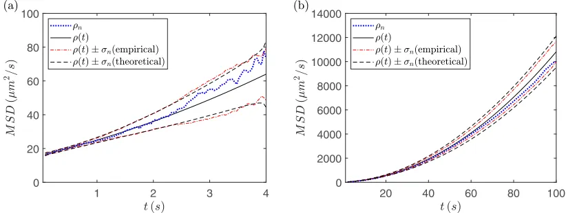
FIG. 1. A plot of the theoretical MSD curve (3) (solid black line), the ensemble time-averaged estimateρn (6) (dotted blue line), along withρ(t)±σn, whereσnis estimated empirically using 10 samples (dot-dashed red line) andρ(t)±σnwhereσnis given by (7) (dashed black line), for a measurement time interval ofT =4 s (a) andT =100 s (b). These experiments were forD=2μm2_{/s,α=1μm/s,η=2μm,} NS =10, andN=100.

To investigate the behavior of the MSD (3) as well as the quality of the ensemble time-averaged estimate (6), simulated data were obtained by solving numerically the drift-diffusion SDE (1) by the Euler-Maruyama method withNS =10

trajec-tories andN =100 time points. Figure1shows a plot of the theoretical MSDρ(t) compared with the estimate ρn. These

experiments were forD=2μm2_{/s,α=1μm/s,η=2μm.} To estimate the uncertainty inρn, Fig.1also includes plots of

ρn±σn. Both the theoreticalσngiven by (7) and an empirical

estimate ofσn, obtained using 10 independent sample values

ofρn, are shown. The plot on the left shows simulations with a

time interval ofT =4 s while the right plot shows simulations with the same parameter values but with a larger time interval T =100 s. We can see that as time increases the size of the uncertainty in ρn increases and for small times ρn does not

approximateρ(t) well. This suggests a sufficiently largeT is required in order to approximate the MSD accurately. We have also observed that choosingT too small lowers the accuracy of inferring the drift velocity, while taking the interval too large lowers the accuracy of inferring the diffusion coeffi-cient. This is due to the quadratic form of the MSD, giving rise to two different timescales for the diffusive and drift processes.

B. Variance of the regression coefficients

Since ρ(t)=a+bt+ct2_{, where a=4η}2_{, b=4D, and} c=α2_{, the coefficients can be inferred by quadratic} regres-sion [23]. Let σ2

n be the variance of ρn at the time point

tn =nT/N, 1nN, and σnm2 =E(ρnρm)−E(ρn)E(ρm)

be the covariance betweenρnandρm, where 1n,mN.

For a quadratic polynomial of the form μ(t)=a+bt+ ct2_{, the variance of the regression coefficients, calculated} by fitting the first p MSD points, can be estimated by [13]

σ2

a ≈

p

n=1

σ2 n ∂a ∂μn 2 +2 p

n=1

n₋1

m=1

σ2 nm ∂a ∂μn ∂a ∂μm ,

3 pN, (8)

σ2

b ≈

p

n=1

σ2 n ∂b ∂μn 2 +2 p

n=1

n₋1

m=1

σ2 nm ∂b ∂μn ∂b ∂μm ,

3pN, (9)

σ2

c ≈

p

n=1

σ2 n _∂c ∂μn 2 +2 p

n=1

n−1

m=1

σ2 nm _∂c ∂μn _∂c ∂μm ,

3pN, (10)

where

∂a

∂μn

=S2S4−S32−S1S4tn+S1S3tn2+S2S3tn−S2₂tn2

σ2

n

, (11)

∂b

∂μn =

S0S4tn−S0S3tn2−S1S4+S2S3+S1S2tn2−S22tn

σ2

n

,

(12)

∂c

∂μn =

S0S2tn2−S0S3tn−S₁2tn2+S1S2tn+S1S3−S22

σ2

n

,

(13)

and

Sk= p

n=1 (tn)k

σ2

n

, k=0, . . . ,4, 3 pN,

=

S0 S1 S2

S1 S2 S3

S2 S3 S4 .

(14)

101 102 10-1

100 101

101 102

0.1 0.2 0.3 0.4 0.5 0.6

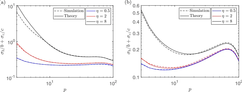
FIG. 2. A plot of the theoretical value ofσb/b+σc/c(solid lines) and its empirically estimated value using 1000 samples (dashed lines) when fit with the firstpMSD points forη=0.5μm, 2μm, and 8μm (from bottom to top, respectively, in both plots) fort=1 s giving

T =100 s (a) andt=10 s givingT =1000 s (b). These experiments were forD=2μm2_{/s,α=1μm/s,N}

S=10, andN=100. The optimal number of fitting points are 100 for all values ofηin (a) and 7, 8, and 100 forη=0.5μm, 2μm, and 8μm, respectively, in (b).

of the MSD is

σ2

nm=

⎧ ⎪ ⎪ ⎪ ⎪ ⎪ ⎪ ⎪ ⎪ ⎪ ⎪ ⎪ ⎪ ⎪ ⎪ ⎪ ⎪ ⎨ ⎪ ⎪ ⎪ ⎪ ⎪ ⎪ ⎪ ⎪ ⎪ ⎪ ⎪ ⎪ ⎪ ⎪ ⎪ ⎪ ⎩

16nD2_(t)2

6KP {−n3−2Pn2+[1−6m2+6(N+1)m]n+2P}

+8α2_(t)3_mn2_D

3KP {−n

2_+3[−m2_{+(N+1)m+1/3]} +}32η2_nDt K

+8η4_(−n+2P)

KP +

8α2_(t)2_mn2_η2 KP

/NS m+nN

8D2_(t)2

3K {−m

3_{+(3+3N−4n)m}2_{+[8(N+1)n−2−3N}2_−6N]m

−6n3+6(N+1)n2−(4N2+8N)n+N(N+2)(N+1)} +8α2_D(t)3_mn

3K [m

2_{−2(N+1)m+3n}2_−3(N+1)nN2_{+2N] m+n>N}

+8η2 K [α

2_(t)2_mn+4Dnt+η2_]/N

S,

(15)

where K=N+1−n and P=N+1−m. Again, in the absence of drift, the covariance (15) is exactly as stated in Michalet [13].

In this paper we are interested in the optimal estimation of the diffusion coefficientDand the drift magnitude α. Since these are related to the regression coefficients b and c, we look to minimizeσb/b+σc/c, the relative errors inbandc.

This can be done in two ways depending on the experimental protocol.

III. RESULTS USING THE OPTIMAL NUMBER OF FITTING POINTS

A. Determination of the optimal number of fitting points

If experiments cannot be repeated, then the optimal esti-mates of the model parameters may be obtained by fitting a subset of the MSD points. For this, we assume that the MSD is calculated using allN time points [as in Eqs. (5) and (6)] and then fit using a subset of these points (see Sec.II B). In the Supplemental Material (section 4.1) we look at optimizing the number of fitting points for different choices ofNS and

N, as well as results for inferring the diffusion coefficient, drift magnitude, and standard deviation of the static error. To investigate optimizing the number of fitting points, we look at the theoretical value of the uncertainty σb/b+σc/c

using (8)–(14) for different values ofpand compare this with an empirical estimate calculated from simulations. For the estimated uncertainty, we calculate the MSD data points then use WLS regression to obtain estimates forbandcby fitting with the first ppoints, where 3pN. This was repeated 1000 times to empirically estimate the values ofσb andσc.

Figure2shows the theoretical and simulated value ofσb/b+

σc/cas a function of the number of fitting points pfor two

differentt values forη=0.5μm, 2μm, and 8μm. These experiments were forD=2μm2_{/s,α=1μm/s,η=2μm,} NS=10, andN =100, witht =1sgivingT =100 s for

Algorithm 1Iterative algorithm to findpoptand estimates ofD,α, andη

Input: MSD data found atNfixed time points with time stept=T/N, and convergence parameterτ. Output: Estimates of optimal number of fitting pointspoptand parametersD,αandη.

1: Set the number of fitting pointsp0=Nand seti=0.

2: ifi=0then 3: σ2 (i)

n =1, 1npi, 4: else

5: σ2 (i)

n =σn2(Di, αi, ηi, t) using (7), 1npi. 6: end if

7: Use WLS regression with weights 1/σ2 (i)

n on the firstpipoints of the MSD to get the parameter estimatesDi,αiandηi. 8: Updatepi+1=popt(Di, αi, ηi, t,N).

9: if(pi+1−pi)/pi+1< τthen

10: end algorithm, 11: else

12: Seti=i+1 and go back to Step 2. 13: end if

that the value ofpopt depends on the model parametersD,α,

andη, as well as the size of the time interval between frames

tand the total number of time pointsN. In the Supplemental Material (section 4.2) we provide a MATLAB routine which determinespopt(D, α, η, t,N) given these input parameters.

B. Iterative algorithm to calculatepopt

The difficulty with using popt(D, α, η, t,N) to infer the model parameters is we require the values of D, α, and η themselves in order to calculate it. We therefore consider the following iterative technique for determining popt. The iterative algorithm initially estimatesD,α, andηby fitting all N MSD points. The weighting used in the fitting is initially taken to be uniform, and then, for all future iterations, we estimate the variance of the MSD by substituting the current parameter estimates into (7). The algorithm then adapts the number of fitting points according to Algorithm1.

The toleranceτ determines the stopping criterion depend-ing on the relative differences between two successive pi

values.

We tested the iterative algorithm for the parameter values

D=2μm2_{/s,α=1μm/s, andη=2μm for three different}

time steps,t =1 s,t =10 s, andt=100 s. Each simu-lation run usesN=1000 time points andNS =10 trajectories

to create the MSD data and a quadratic fit. Since simulations are likely to end after a different number of iterations, Steps 9– 11 of Algorithm1will be ignored and instead all simulations are stopped after 10 iterations. These simulations were then repeated 100 times. By denoting the mean value of a quantity by the angular brackets·we indicate the performance of the algorithm by plottingpi,|Di/D−1|, and|αi/α−1|in

Fig.3. The first thing to notice is that the algorithm converges to popt in a couple of iterations for the cases considered, with most being after just one iteration. We do not see much improvement in|αi/α−1|when fit with the optimal

number of fitting points, compared with all the MSD points, for any value of t. However, we do see a decrease in its value as we increase t. This is due to the value of the measurement time intervalT increasing as we increaset. This increase inT moves us into the drift timescale where the

inference ofαis better. The value of|Di/D−1|decreases

after one iteration in all cases, with a larger decrease for larger values oft. The final value of|Di/D−1|decreases

when t =1 s is increased tot=10 s but then increases fort =100 s. Here a small value oft, corresponding with a small value ofT, is likely to give data which is static error dominated. When we increaset we leave the noisy domain and so the inference of Dis improved. However, when we increaseT too much, we leave the diffusive timescale and so the inference ofDbegins to deteriorate. This example shows that the choice of t is important for the optimal inference of both the parameters. Additional experiments were run for different values ofD andα, which can be found in the Supplemental Material (section 4.3).

C. Single-particle parameter estimation usingpopt

While the analysis and results presented so far assume the availability of data for an ensemble of particles, in some situations only single-particle data are available. We now consider how the results we have perform in the single-particle case. An important point to note is that the optimal number of fitting points for both the single-particle case and ensemble of particles case are identical. This is because when calculating the variance and covariance of the MSD in the ensemble particle case, we simply take the single-particle variance and covariance and divide byNS, as stated in the Supplemental

Material (sections 2 and 3). Hence, when calculating the variance of the regression coefficients in (8)–(10), for the ensemble case, we can take out a factor of 1/NS fromσn2and

σ2

nm. Therefore, the value ofσb/b+σc/cin the ensemble case

will be a factor of√NS smaller than the single-particle case

2 4 6 8 10

Iteration

100 101 102 103

2 4 6 8 10

Iteration

10-4 10-3 10-2 10-1 100

Relative Error

2 4 6 8 10

Iteration

100 101 102 103

2 4 6 8 10

Iteration

10-4 10-3 10-2 10-1 100

Relative Error

2 4 6 8 10

Iteration

100 101 102 103

2 4 6 8 10

Iteration

10-4 10-3 10-2 10-1 100

Relative Error

FIG. 3. A plot of the value ofpifor each iteration with standard error bars [(a), (c), and (e)], along with a plot of the value of|Di/D−1| (red crosses) and|αi/α−1|(blue circles) for each iteration with standard error bars [(b), (d), and (f)] fort=1 s [(a) and (b)],t=10 s [(c) and (d)], andt=100 s [(e) and (f)]. These experiments were forD=2μm2_{/s,α=1μm/s,η=2μm,N}

S =10, andN=1000. The dashed line in the plots ofpicorrespond topopt=50 (a),popt=16 (c), andpopt =7 (e), while the dashed line in the plots of|Di/D−1| and|αi/α−1|correspond with the value 10−2, indicating a 1% error.

Figure4shows the results of the iterative algorithm for the same parameter values as in Fig.3but forNS =1. Since we

only have a single particle, we expect the relative errors to be higher. Therefore, in each right plot, the dashed line will now correspond to a 10% error. Notice that the value ofpitakes a

couple more iterations to converge but still does so in a small number of iterations. We often see the relative errors converge beforepi, which is a result of the shallow minimum around

popt in the right plot of Fig.2. We have also observed similar behavior for repeatable experiments; for example, Figs. 5

and 7. We see the same trend for |αi/α−1| as before,

namely that fitting with the optimal number of fitting points does not improve its value much, but using a large value of t does. However, we see that the value of |Di/D−1|

2 4 6 8 10

Iteration

100 101 102 103

2 4 6 8 10

Iteration

10-4 10-2 100 102

Relative Error

2 4 6 8 10

Iteration

100 101 102 103

2 4 6 8 10

Iteration

10-4 10-2 100 102

Relative Error

2 4 6 8 10

Iteration

100 101 102 103

2 4 6 8 10

Iteration

10-4 10-2 100 102

Relative Error

FIG. 4. A plot of the value ofpifor each iteration with standard error bars [(a), (c), and (e)], along with a plot of the value of|Di/D−1| (red crosses) and|αi/α−1|(blue circles) for each iteration with standard error bars [(b), (d), and (f)] fort=1 s [(a) and (b)],t=10 s [(c) and (d)], andt=100 s [(e) and (f)]. These experiments were forD=2μm2_{/s,α=1μm/s,η=2μm,N}

S=1, andN=1000. The dashed line in the plots ofpicorrespond topopt=50 (a),popt=16 (c), andpopt =7 (e), while the dashed line in the plots of|Di/D−1| and|αi/α−1|correspond with the value 10−1, indicating a 10% error.

IV. RESULTS USING THE OPTIMAL MEASUREMENT INTERVAL

A. Determination of the optimal measurement time interval

If experiments are able to be repeated then the optimization can be done with respect to the measurement time interval T rather than the number of MSD fitting points. This has the advantage that the optimal measurement time interval could help inform future experiments. For this method we

assume that the MSD is calculated from all N time points and that all ρn data points are used in the fitting process.

Note that since all the MSD points are used in the fitting, a new value ofT will correspond with a new value oft. As stated before we concentrate on the optimal inference of the diffusion coefficient and drift magnitude. In the Supplemental Material (section 5.1) we again present similar results for different choices ofNS andN, as well as results for inferring

100 105 10-1

100 101

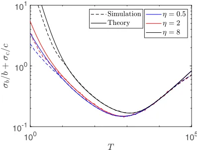
FIG. 5. A plot of the theoretical value of σb/b+σc/c (solid lines) and its empirically estimated value using 1000 samples (dashed lines) against many different values ofT forη=0.5μm, 2μm, and 8μm (bottom to top, respectively). These experiments were forD=2μm2_{/s,α=1μm/s, N}

S =10 andN=100. For

η=0.5μm, 2μm, and 8μm, the optimal measurement time inter-vals areTopt≈735 s, 780 s, and 1216 s, respectively.

Here, the theoretical uncertaintyσb/b+σc/cis calculated

over many different values ofT using (8)–(14) with p=N so that all the MSD points are used in the fitting, and is com-pared with simulations. The simulated result was found by calculating the MSD and using WLS regression to obtain es-timates ofbandc. This was repeated 1000 times to obtain es-timates ofσbandσc. Figure5shows the comparison between

the theoretical and simulated value ofσb/b+σc/cover many

different values ofT forη=0.5μm, 2μm, and 8μm. These experiment were for D=2μm2_{/s, α=1μm/s, N}

S =10,

andN =100. We denote the value ofT which minimizes the uncertaintyσb/b+σc/cbyTopt. We can see that we have good

agreement between the theory and simulated uncertainties, more so closer to Topt. We also see that for all the cases tested, there exists an optimal measurement time interval. For

η=0.5μm, 2μm, and 8μm these optimal measurement

time intervals are Topt≈735 s, 780 s, and 1216 s. In the Supplemental Material (section 5.2) we provide a MATLAB

routine which determines Topt(D, α, η,N) given the input parameters.

B. Iterative algorithm to calculateTopt

As before, the function to calculate Topt depends on the model parameters and so another iterative algorithm was cre-ated. Note that each new iteration corresponds with repeating the experiment with a new measurement time intervalTi. To

begin the iteration we need to provide an initial guess forTopt, which we denote by T0, with time interval between frames t0=T0/N. The algorithm then adapts the time according to Algorithm2.

The role of the under-relaxation parameterωiis to improve

the robustness of the algorithm by reducing oscillations; this is effectively a low-pass filter for the time series of adjustments. For example, if the initial guess T0 is far from the optimal valueTopt, then the valuesTi will quickly be adapted toward

the optimal time. Close to the optimal time the algorithm can display oscillations in the convergence behavior, i.e., (Ti+1− Ti)×(Ti−Ti−1)<0. When this occurs the relaxation param-eterωi is decreased to smooth out the difference between

it-erates. The toleranceτ determines when to stop the algorithm depending on the relative differences between two successive time points. The rate at which the value of ωi is decreased

in Step 10 is determined by the adjustment parameter ψ where 0< ψ 1. In the experiments that follow, the value of ψ=0.8 has been used but additional values ofψwere tested in the Supplemental Material (section 5.3).

Algorithm 2Iterative algorithm to findToptand estimates ofD,α, andη

Input: Initial estimate of measurement time intervalT0and measurement interval between framest0, number of time pointsN,

adaptation parameterψand convergence parameterτ.

Output: Estimates of optimal timeToptand parametersD,αandη.

1: Guess an initial timeT0with correspondingt0and set the relaxation parameterω0 =1 and seti=0.

2: ifi=0then 3: σ2 (i)

n =1, 1nN, 4: else

5: σ2 (i) n =σ

2

n(Di, αi, ηi, ti) using (7), 1nN. 6: end if

7: Calculate the MSD at theNtime points with intervaltiup toTiand use WLS on all the points with weights 1/σ2 (i)

n to get the parameter estimatesDi,αiandηi.

8: UpdateTi+1=(1−ωi)Ti+ωiTopt(Di, αi, ηi,N) and calculateti+1=Ti+1/N.

9: ifi2 and (Ti+1−Ti)×(Ti−Ti−1)<0then

10: ωi+1=ψ×ωi, 0< ψ1 11: else

12: ωi+1=ωi 13: end if

14: if(Ti+1−Ti)/Ti+1< τthen

15: end algorithm 16: else

2 4 6 8 10

Iteration

102 104 106

2 4 6 8 10

Iteration

10-4 10-2 100 102

Relative Error

2 4 6 8 10

Iteration

10-2 100 102 104

2 4 6 8 10

Iteration

10-2 100 102 104

Relative Error

FIG. 6. A plot of the value ofTifor each iteration with standard error bars [(a) and (c)], along with a plot of the value of|Di/D−1| (red crosses) and|αi/α−1|(blue circles) for each iteration with standard error bars [(b) and (d)]. These experiments were forD=2μm2/s,

α=1μm/s,η=2μm,NS =10, andN=100, with a starting time ofT0=107s [(a) and (b)] andT0=10−3s [(c) and (d)]. The dashed line

in the plots ofTicorrespond toTopt≈780 s, while the dashed line in the plots of|Di/D−1|and|αi/α−1|correspond with the value 10−1_{, indicating a 10% error.}

The iterative algorithm was tested for the two different ini-tial measurement time intervals,T0=107s andT0 =10−3s. Both experiments were for D=2μm2_{/s, α=1μm/s,} η=2μm, NS =10, and N=100; for these parameters

Topt≈780 s. Again, Steps 14–16 of Algorithm 2 will be ignored and instead all simulations are stopped after 10 itera-tions. These simulations were then repeated 100 times. The quantities Ti, |Di/D−1|and |αi/α−1| are shown in

Fig.6. Notice that the initial guessT0=107s significantly overestimates the true value ofTopt, but that the value ofTi

converges rapidly to a value close to Topt. While the value of |αi/α−1| becomes less accurate as we progress, the

value of |Di/D−1| quickly falls from around a 1000%

error to under a 10% error in a small number of iterations. When using a much smaller initial time ofT0=10−3s, we see that Ti still converges to Topt in a small number of iterations. Initially the value of |Di/D−1| is of the

or-der of magnitude 102 _{while |α}

i/α−1| is of the order of

magnitude 103_{, corresponding to a 10 000% and 100 000%} error, respectively. This highlights the fact that an incorrect choice ofT can lead to very large inaccuracies in the value of inferred parameters. However, using the adaptive algorithm we see that as theTivalues get closer toTopt, the errors both reduce to under 10%. This stresses the importance of using

Topt when inferringDandαusing all the MSD points in the fitting. Additional experiments were run for different values ofDandα, which can be found in the Supplemental Material (section 5.3).

C. Single-particle parameter estimation usingTopt

The results for Topt can also extend to the single-particle case for the same reasons as the popt method. The optimal measurement time interval will be the same for an ensemble of particles and the single-particle cases. Figure7 compares the performances using the same initial measurement time intervals, T0=107s and T0=10−3s, for the same param-eter values as those in Fig. 6 but with NS=1. The value

of Ti continues to converge in a small number of

itera-tions and we observe that the results for |Di/D−1| and

|αi/α−1| have similar dynamics to the ensemble case.

These show the strength of the iterative algorithm as they give good results even in the single-particle case where we have less information. Further experiments for different values of D and α can be found in the Supplemental Material (section 5.4).

2 4 6 8 10

Iteration

100 102 104 106

2 4 6 8 10

Iteration

10-4 10-2 100 102 104

Relative Value

2 4 6 8 10

Iteration

100 105

2 4 6 8 10

Iteration

10-2 100 102 104

Relative Value

FIG. 7. A plot of the value ofTifor each iteration with standard error bars [(a) and (c)], along with a plot of the value of|Di/D−1| (red crosses) and|αi/α−1|(blue circles) for each iteration with standard error bars [(b) and (d)]. These experiments were forD=2μm2/s,

α=1μm/s andη=2μm,NS =1 andN=100, with a starting time ofT0=107s [(a) and (b)] andT0=10−3s [(c) and (d)]. The dashed

line in the plots ofTicorrespond toTopt≈780 s, while the dashed line in the plots of|Di/D−1|and|αi/α−1|correspond with the value 10−1_{, indicating a 10% error.}

application domain. For instance, in environmental statistics, where the task is, e.g., to monitor the spread of pollutants and contaminants in ground water, it is common practice to repeatedly estimate the same physical quantities. This setting therefore naturally lends itself to the integration of the pro-posed iterative adjustment scheme. For other applications, like the study of collective cell movement with high-resolution microscopy, a change of the experimental protocol may be required to allow (and budget) for a series of experiments that enable iterative adjustments of the measurement time intervals.

V. DISCUSSION

A. Fitting method

Throughout the paper we assume that WLS regression is used to infer the parameters of the model. Michalet [13] showed that, in the absence of drift, the uncertainty in the parameters when using WLS and ordinary least squares (OLS) were similar as long as the optimal number of fitting points were used. When drift is included we find that WLS gives bet-ter results, both for using the optimal number of fitting points and the optimal measurement time interval, as shown in Fig.8. We can see that in all cases using WLS gives better results

than using OLS. When fitting with a subset of the MSD points, corresponding to the top plots, we do not have a big difference in the minimal uncertainty between WLS and OLS, but when optimizing the measurement time interval, corresponding to the bottom plot, we see a significant difference, with WLS being almost an order of magnitude better.

B. Initial parameter estimates

Our analysis has shown that the optimal number of fitting points or the optimal measurement time depend on the quan-tities of interest themselves—the diffusion coefficientDand the drift magnitudeα−via

popt=popt(D, α, η, t,N) and Topt = Topt(D, α, η,N). (16)

101 102 0.2

0.4 0.6 0.8 1 1.2 1.4

101 102

10-1 100

100 105

10-1 100 101 102

FIG. 8. A plot of an empirically estimated value ofσb/b+σc/cusing WLS (solid red line) and OLS (dashed black line) as a function of the number of fitting points [(a) and (b)] or fit with all the MSD points over a number of measurement time intervals (c). These experiments were forD=2μm2_{/s,α=1μm/s,η=2μm,N}

S=10, andN=100. For the plots using the number of fitting points we have thatt=1s givingT =100 s (a) andt=10 s givingT =1000 s (b).

and p(η). From this, we can derive the prior expectation of Topt:

T_opt0 =

Topt(D, α, η,N)p(D)p(α)p(η)dDdαdη,

which in practice can be estimated with a Monte Carlo sum:

T_opt0 = 1 M

M

i₌1

Topt(D, α, η,N),

where (αi,Di, ηi) are independent draws fromp(α)p(D)p(η)

with sample sizeM. This provides a good initial guess for the unknown optimal timeTopt. A similar procedure could be used to generate an initial estimate forpopt.

C. Practical considerations in applications

An implicit assumption on which the proposed methodol-ogy is based is that of complete observation. This may not be valid in a real experiment, with missing values caused, e.g., by fluorophore bleaching. If the proportion of missing values is small, and values are missing at random, then there are established statistical procedures based, e.g., on the

A further assumption has been that the advection-diffusion model of Eq. (1) provides an accurate mathematical descrip-tion of the true process under investigadescrip-tion. This may not be the case, e.g., due to inhomogeneities in the medium, leading to a more complex spatial distribution of the advection and diffusion parameters. In addition, there has recently been much interest in modeling animal movement (e.g., Hooten et al. [25]) and cell movement (e.g., Jones et al. [2]) with advection-diffusion type processes. However, in these cases we are not dealing with genuine physical processes but with more complex biological processes that merely exhibit similar characteristics. So an important question is that of model critique, i.e., to establish whether the assumed mathematical process provides an adequate description of the observed data. To this end, one can choose from a series of statistical techniques, ranging from computationally cheap asymptotic methods, like chi-square and G tests (e.g., McDonald [26]), to computationally more expensive nonasymptotic procedures, like the parametric bootstrap [27,28]. However, what all these methods have in common is the assumption of a reliable procedure for accurate parameter estimation in the assumed model, as otherwise a correct or adequate model may be rejected erroneously. Hence any form of model critique will greatly benefit from the improved parameter estimation pro-cedure proposed in the present paper.

There are many scenarios where we want to discriminate between alternative models based on the observed data. For instance, we may want to establish whether the system of interest is subject to advection as opposed to be driven by diffusion only. In other scenarios, we may want to know if there are significant other driving forces in the system in addition to advection and diffusion. Since these models are nested, one can fit the MSD data and then use an F-test to test the null hypothesis that the data have arisen from the simpler model. Again, the procedure is based on the assumption that the model parameters have been estimated accurately. As we

have shown, this depends strongly on how the MSD data are fitted, and the proposed procedure for variance reduction makes a important contribution here.

VI. CONCLUSIONS

When particles are assumed to undergo Brownian motion with drift, and the measured position of the particles is subject to static localization error, the accurate inference of model parameters is dependent on either the number of MSD points used in the WLS fitting or the measurement time interval, depending on the experimental protocol. In both cases, when T is too small we get inaccurate estimates for the drift magnitude, as well as the data being dominated by the static error, while larger values ofT result in inaccurate inference of the diffusion coefficient. For experiments which cannot be repeated, an optimal number of fitting points popt was found which optimized the inference of the model parameters. Sim-ilarly, for repeatable experiments, an optimal measurement time intervalTopt was found. Both popt andTopt depended on the parameters themselves and so an iterative algorithm was created for both procedures which gives optimally accurate estimates of the parameters. This depended on the calculation of an analytical form for the variance and covariance of the time-average overlapping MSD, particularly the variance as this could be used to perform WLS in the single-particle case.

ACKNOWLEDGMENTS

This work was funded by CRUK, Grant No. C22713/A21462, and the UK Engineering and Physical Sciences Research Council (EPSRC), Grant No. EP/N014642/1, as part of the SofTMech project. Dirk Husmeier is supported by a grant from the Royal Society of Edinburgh, Award No. 62335.

[1] E. A. Ferguson, J. Matthiopoulos, R. H. Insall, and D. Husmeier,J. Roy. Stat. Soc. C66,869(2017).

[2] P. J. Jones, A. Sim, H. B. Taylor, L. Bugeon, M. J. Dallman, B. Pereira, M. P. Stumpf, and J. Liepe,Phys. Biol.12,066001 (2015).

[3] E. A. Ferguson, J. Matthiopoulos, R. H. Insall, and D. Husmeier,J. Roy. Soc. Interface13(2016).

[4] M. B. Hooten, D. S. Johnson, B. T. McClintock, and J. M. Morales, Animal Movement: Statistical Models for Telemetry Data(CRC Press, Boca Raton, FL, 2017).

[5] D. Helbing, A. Johansson, and H. Z. Al-Abideen,Phys. Rev. E 75,046109(2007).

[6] C. Burstedde, K. Klauck, A. Schadschneider, and J. Zittartz, Physica A295,507(2001).

[7] M. T. Thai, W. Wu, and H. Xiong,Big Data in Complex and Social Networks(CRC Press, Boca Raton, FL, 2017).

[8] T. Savin and P. Doyle,Biophys. J.88,623(2005). [9] C. L. Vestergaard,Phys. Rev. E94,022401(2016).

[10] H. Qian, M. Sheetz, and E. Elson,Biophys. J.60,910(1991). [11] M. Saxton and K. Jacobson, Annu. Rev. Biophys. Biomol.

Struct.26,373(1997).

[12] M. Saxton,Biophys. J.72,1744(1997). [13] X. Michalet,Phys. Rev. E82,041914(2010). [14] A. J. Berglund,Phys. Rev. E82,011917(2010).

[15] X. Michalet and A. J. Berglund, Phys. Rev. E 85, 061916 (2012).

[16] S. Shanbhag,Phys. Rev. E88,042816(2013).

[17] E. M. Tang and P. T. Underhill, Langmuir 34, 10694 (2018).

[18] H. Taylor, J. Liepe, C. Barthen, L. Bugeon, M. Huvet, P. Kirk, S. Brown, J. Lamb, M. Stumpf, and M. Dallman,Immunol. Cell Biol.91,60(2013).

[19] E. Banigan, T. Harris, D. Christian, C. Hunter, and A. Liu,PLoS Comput. Biol.11,1(2015).

[20] M. Saxton,Biophys. J.67,2110(1994).

[21] See Supplemental Material athttp://link.aps.org/supplemental/ 10.1103/PhysRevE.100.022134 for all mathematical deriva-tions, further experiments with different parameter choices, and results with the inclusion of motion blur and inferring the drift angle.

[23] P. Bevington and D. Robinson, Data Reduction and Error Analysis for the Physical Sciences(McGraw–Hill, New York, 2003).

[24] A. P. Dempster, N. M. Laird, and D. B. Rubin,J. Roy. Stat. Soc. B39,1(1977).

[25] M. B. Hooten, D. S. Johnson, B. T. McClintock, and J. M. Morales, Animal Movement: Statistical Models for Telemetry Data(CRC Press, Boca Raton, FL, 2017).

[26] J. H. McDonald, Handbook of Biological Statistics, Vol. 2 (Sparky House Publishing, Baltimore, MD, 2009), pp. 53–58.

[27] B. Efron and R. J. Tibshirani,An Introduction to the Bootstrap

(CRC Press, Boca Raton, FL, 1993).