Data Abstraction for Visualizing Large Time Series

City, University of London Institutional Repository

Citation:

Shurkhovetskyy, G., Andrienko, N., Andrienko, G. & Fuchs, G. (2017). Data

Abstraction for Visualizing Large Time Series. Computer Graphics Forum, doi:

10.1111/cgf.13237

This is the accepted version of the paper.

This version of the publication may differ from the final published

version.

Permanent repository link:

http://openaccess.city.ac.uk/17818/

Link to published version:

http://dx.doi.org/10.1111/cgf.13237

Copyright and reuse: City Research Online aims to make research

outputs of City, University of London available to a wider audience.

Copyright and Moral Rights remain with the author(s) and/or copyright

holders. URLs from City Research Online may be freely distributed and

linked to.

Eurographics Conference on Visualization (EuroVis) 2016 K-L. Ma, G. Santucci, and J. J. van Wijk

(Guest Editors)

(2016),

Data Abstraction for Visualizing Large Time Series

G. Shurkhovetskyy1,N. Andrienko2,3,G. Andrienko2,3,and G. Fuchs2

1_{University of Bonn, Germany} 2_{Fraunhofer Institute IAIS, Germany}

3_{City University London, UK}

Abstract

Numeric time series is a class of data consisting of chronologically ordered observations represented by numeric values. Much of the data in various domains, such as financial, medical, and scientific, are represented in the form of time series. To cope with the increasing sizes of datasets, numerous approaches for abstracting large temporal data are developed in the area of data mining. Many of them proved to be useful for time series visualization. How-ever, despite the existence of numerous surveys on time series mining and visualization, there is no comprehensive classification of the existing methods based on the needs of visualization designers. We propose a classification framework that defines essential criteria for selecting an abstraction method with an eye to subsequent visualiza-tion and support of users’ analysis tasks. We show that approaches developed in the data mining field are capable of creating representations that are useful for visualizing time series data. We evaluate these methods in terms of the defined criteria and provide a summary table that can be easily used for selecting suitable abstraction methods depending on data properties, desirable form of representation, behavior features to be studied, required accu-racy and level of detail, and the necessity of efficient search and querying. We also indicate directions for possible extension of the proposed classification framework.

Categories and Subject Descriptors (according to ACM CCS): I.3.3 [Computer Graphics]: Picture/Image Generation—Line and curve generation

1. Introduction

Time series are a type of data that can be found frequently in observation of real world phenomena in financial, medi-cal, engineering, scientific, social and military applications. Interest in time series analysis has been present for several decades, if not centuries.

In many settings, the human eye is the most reliable tool for analyzing large data [Kei02]. Therefore, appropriate rep-resentation of time series is the foundation for efficient task solving. Many data mining tasks can be facilitated by vi-sualization of the data. There is a bidirectional relationship between visualization of time series and corresponding data mining tasks. The majority of tasks mentioned in a survey on time series mining [Fu11] and associated methods de-signed to solve them are helpful in creating efficient visu-alizations. At the same time, efficient visualizations enhance the task solving process for many of the known mining tasks. For instance, visualization and interaction with data facil-itates search for optimal parameterization of complex

sys-tems, and increases chances of arriving at results that are close to optimal [CRC03]. This is particularly the case when advanced analytical algorithms are applied, whose tuning is only possible with good understanding of their work princi-ples [SK13].

However, the massive size of many contemporary data sets pose significant challenges to both visualization and analysis [DSP∗17,Fek13]. Often, time series data are so large that it becomes either infeasible or useless to display them all. Attempts to do so result either in unresponsive dis-plays or in cluttered visualizations that are impossible to read and do not allow extracting any meaningful informa-tion. Analysis algorithms, in turn, might degrade in perfor-mance. One way to diminish such effects is to rely on data abstraction. Representing datasets at hand in a form that is significantly smaller in size while preserving features impor-tant for the user is the ultimate goal of abstraction of any type of data, including temporal.

principal approaches to data abstraction, aggregation- and feature-based. The former assumes calculating aggregated data values for portions of data and visualizing these ag-gregates. The latter is based on showing only those parts of the data that satisfy certain preset criteria, which supposedly characterize chunks of data the user deems interesting, or that are important in the context of the analysis task at hand. The task of time series abstraction for visualization has been addressed by many researchers who introduced diverse methods for solving the problem. In general, the problem can be addressed in two ways: reducing the length (from here on, by length we refer to the number of time steps in a single series), and reducing the number of time series in cases when there are multiple series to be dealt with.

Time series mining is an active area of research in data mining and knowledge discovery that produced, among oth-ers, numerous abstraction methods for time series. To the best of our knowledge, there have yet been no attempts to systematically review these methods from the perspective of visualization and visual analytics. Logically, the first step to good visualization design for large time series is the se-lection of a suitable abstraction algorithm that can facilitate users’ perception and analysis. This work aims at laying the foundations for such a selection.

Achieving this aim involves two sub-goals: first, deter-mine the relevant criteria for the selection of an abstraction method, and second, evaluate the existing abstraction meth-ods in terms of these criteria. A starting point towards the first sub-goal is the consideration of two aspects: the possi-ble properties of thedata(i.e., time series) that need to be abstracted, and the intendedanalysis tasks. The first aspect relates to the applicability of methods while the second as-pect refers to the utility of method results, i.e., whether the transformed data can effectively support the intended tasks.

The main contribution of this paper is providing navi-gation for visual analysts through a systematic inventory of available abstraction methods. Systematization driven by user analysis goals and informed by requirements for en-abling visualization tasks is exactly what the visualization community has been advocating [BL10,AMM∗08a,BL09,

KMS∗08].

This paper is organized as follows. In Section2, we in-troduce the problem of visualizing large time series, explain the need for using abstraction, and define the scope of our work. Section3provides an overview of the related work. Section4describes our classification framework. We intro-duce and substantiate the proposed criteria for classifying and choosing abstraction techniques. In Section5, represen-tative methods for time series abstraction resulting from re-search in the field of data mining are evaluated in terms of these criteria. We continue with a discussion of how analysts can benefit from our classification framework and method survey in Section6. Section7suggests possible research di-rections for extending the proposed framework with

addi-tional potentially relevant criteria. It is followed by a con-clusion in Section8.

2. Background 2.1. Time Series

A time series in general form is a data type represented by an ordered sequence of observations, where an observation is represented by a specific value of some attribute or a combi-nation of values of several attributes, orvariables, the latter term being typically used in statistics and data mining. In this paper, we focus on numeric-valued variables. A time series comprising values of a single variable is calledunivariate. A univariate time series of lengthT can be represented as

x(t) =x(1)...x(t)...x(T). A time series comprising values of several variables is calledmultivariate. A multivariate time series withNvariables can be represented byNper-variable univariate time series with a common temporal domain. In literature, data with multiple variables are also referred to as

multidimensional, the variables are calleddimensions, and the number of variables in data is called thedimensionality

of the data.

Multivariate (multidimensional) time series need to be distinguished from multiple univariate time series sharing the same variable. For example, a time series of weather pa-rameters, including the temperature, wind speed, wind di-rection, and precipitation, is a multivariate time series in which each weather parameter is represented by one vari-able. Multiple time series of measurements of the same pa-rameter, such as the temperature, taken at different locations is an example of multiple univariate time series with a com-mon variable. These two cases require different approaches to the analysis and to the abstraction. Thus, multiple univari-ate time series can be clustered by similarity, which makes no sense for time series with the variables differing in their meanings, measurement units, and value ranges.

Numeric time series make a subclass of a larger class of data calledtime-oriented[AMST11] ortime-referenced

[AA05]. The latter term indicates that data consist of items referring to moments or intervals in time. The data items may not only be scalar values but also events [DSP∗17], graphs [vdEHBvW16], images [BSH∗16a], spatial distribu-tions [AAB∗10], or positions of moving objects [AA17]. Time-referenced data characterize processes and phenomena that vary in time and may be thus calledtime-variant.

oldest example dates back to the tenth century. The set of techniques used to visualize time series has been notably expanded in recent decades by sophisticated approaches like ThemeRiver [HHWN02], calendar-based visualizations [VWVS99], spiral visualizations [WAM01], stacked graphs [BW08], horizon graphs [HKA09], time curves [BSH∗16b], to name a few. A visual survey of time series visualiza-tions compiled by Aigner et al. [AMM∗08a] can be found athttp://survey.timeviz.net.

2.2. Need and Requirements for Time Series Abstraction

When it comes to visualization, there are several conditions that must be taken into consideration when dealing with large time series. First, displaying the entire raw data on a commodity screen (rarely larger than 32 inches diagonally or having resolution greater than 4K) almost certainly re-sults in a cluttered view, which will be of very little utility to a user whose understanding of the data will be hindered. For instance, using a FullHD display that has a horizontal res-olution of 1920 pixels to visualize time series of more than 1920 time steps as a line chart creates the problem of accom-modating more than one time step in every pixel column.

Second, massive amounts of data, if presented in their raw form, may overtax computing resources resulting in unac-ceptably slow responsiveness of the system. Abstraction is used to avoid or at least mitigate these issues [EF10].

The main goal of creating an abstraction is simplification, which means removing unnecessary details and/or extract-ing only important information (i.e., relevant to the analy-sis goals). Simplification involves generating a new, usually smaller in size, representation of given time series. Esling and Agon [EA12] define such a representation as "a model of original time series of reduced dimensionality such that the model closely approximates original time series", where the term ’dimensionality’ refers to the length of the time series, i.e., the number of time steps in it. Simplification is done with the aim to ease processing, querying, and ultimately, visualization.

Shahar [Sha97a] defines temporal abstraction as "a pro-cess which, given a set of time-stamped parameters, exter-nal events and abstraction goals, produces abstractions of the data and interpret past and present states and trends that are relevant for the given set of goals". This definition empha-sizes two things: (1) an abstraction must preserve important features, such as states and trends; (2) what features are im-portant depends on the goals (in other words, analysis tasks). The general requirements for data algorithms aimed at dealing with large data sets and use approximate representa-tions of original data have been outlined by Faloutsos et al. [FRM94] as follows:

• they must be accurate despite the constraint of working with approximate representation of data;

• they must be carried out in main memory thus avoiding disk I/O overhead which is the principal bottleneck of any data-intense operation;

• they must be fast (i.e., computationally efficient). The same requirements must hold in the context of visu-alization. That is, an abstracted data representation must not limit users in their actions required for analysis, nor nega-tively affect their interpretation of data. As stated by Falout-sos et al. [FRM94], it is acceptable for an algorithm (and thus potentially for a visualization, too) to result in false ini-tial findings since they can (hopefully, rapidly) be discarded in later steps. But it is unacceptable if an algorithm or ab-stracted data visualization results in missing potentially use-ful findings.

The latter problem is of particular importance when pro-ducing aggregated or abstracted visualizations of data. It also strongly affects the choice of algorithms one would use for achieving this very abstraction. For instance, in some appli-cations it might be necessary to preserve peaks of time series in their original form, or at least so that maximal values are never altered even in an aggregated view.

2.3. Data Space vs Visual Space Abstractions

Cui et al. [CWRY06] classify abstraction approaches into two groups, namely, abstraction indata spaceand abstrac-tion invisual space. Their classification corresponds to the notion of an Information Visualization Pipeline [CMS99,

Chi00]. Abstraction methods that operate in visual space are zooming [BSH94] and distortion [KLS00].

Keim [Kei02] provides a overview of various abstraction techniques including those operating in visual space.

Our focus is on abstraction in data space. Generally, data abstraction approaches include sampling [DE02], clustering [DGM97], segmentation [cFlCCm06], projection [Tor52], dimensionality reduction (i.e., reducing the number of vari-ables) [YYS05], and others. However, these generic classes of methods may not be straightforwardly applicable to time series. Abstraction of time series requires specific ap-proaches that respect the nature of this data type, partic-ularly, the presence of temporal ordering relationships be-tween the data items. Such approaches are developed in the field of data mining with the aim on generating representa-tions of time series that are to be processed and analyzed by algorithms. In visualization, they can be used to per-form abstraction of data prior to its visual mapping and dis-play [LKL05].

2.4. Scope

In this paper, we review and systematize data abstraction methods that generate simplified representations of time se-ries (the termstime series simplificationandtime series ab-stractionare used interchangeably), which can be useful for visualization purposes. We do not attempt to survey visual-ization methods or visual mappings of time series data. Thus, our focus is on transformations that occur in the early stages of the InfoVis Pipeline [CMS99,Chi00]. We pay particular attention to the temporal nature of time series critical for visualizing and analyzing such temporal data [AMM∗08b]. Figure1summarizes the scope of our paper. In the next sec-tion we discuss other research in the area covered, and ex-plain differences to, and contribution of, our paper. 3. Related Work

We structure the overview of the related works according to the topics and different foci of the publications:

• papers discussing the use of abstraction for visualization in general;

• papers proposing conceptual frameworks for time and time-referenced data;

• papers focusing primarily on visualization of time series but mentioning the use of abstraction;

• papers describing methods for time series transformation. 3.1. Data Abstraction in Visualization

A taxonomy for abstraction in information visualization is proposed by Ellis and Dix [ED07]. The authors do not distin-guish between approaches that operate in data space versus visual space and devote more attention to visual methods. They give an overview of benefits and drawbacks of vari-ous clutter reduction techniques, but consider only general methods and not any data type-specific transformations.

Elmqvist and Fekete [EF10] propose a formal model for data abstraction in visualization, survey existing techniques, and derive guidelines for designing new ones. However, their focus is on hierarchical data aggregation rather than all pos-sible abstractions in data space. Since only one abstraction technique is considered (aggregation), no mapping between techniques and data properties or user tasks is provided.

Du et al. [DSP∗17] introduce an empirically derived tax-onomy of analytical focusing strategies, that is, the ways in which users of visualization tools can interactively simplify the contents of a visual display and extract relevant informa-tion from it. The strategies include extracinforma-tion of data sub-sets, pattern simplification (e.g., by grouping and merging), and partitioning. This work differs from ours mainly in two respects. First, it deals with a different type of data, namely, sequences of events, rather than numeric time series. The simplification methods described are not directly applicable to time series. Second, it describes interactive methods of

simplification, which are applied by users manipulating a vi-sual display. Our paper discusses automatic methods of time series abstraction. The abstraction is supposed to be made prior to visualization by a visualization designer rather than end users.

3.2. Conceptualization of Time

Frank [Fra98] proposes a conceptual model that distin-guishes between different types of time:

• ordinal time:time points happening one after another.

• interval time:every time point (event) is measured on an interval scale and has a length (duration).

• cyclic time:description of cyclic processes for whom ap-plication of an ordered relation is meaningless.

• branching time: events (even same ones) can occur in different branches (alternatives) that describe several sce-narios or processes.

Although Frank suggests different approaches to visual-ize and analyze data based on their types, and his taxonomy provides a solid foundation of categorizing methods for an-alyzing temporal data, it is too general and falls short in the attempt to further classify types of tasks and possible meth-ods in each of the derived categories. Despite the fact that the majority of approaches for visualizing time-referenced data consider ordered time (according to Frank’s taxonomy), his work does not investigate this type any deeper than less com-mon types of time that he describes.

3.3. Visualization of Time-referenced Data

Figure 1:Scope of this survey with regard to the main stages of the information visualization pipeline [CMS99,Chi00]. In contrast to previous state of the art reports (STAR) [LMW∗15], we provide a refined view of a specific stage of the visualization generation process, specifically, the data transformation stage as shown on the diagram. We further narrow our focus by selecting time series data as the source, and develop our systematization according to properties of temporal data.

when elaborating on analytical methods the authors distin-guish between temporal data abstraction, principal compo-nent analysis and clustering, leaving out a variety of other approaches to obtaining abstracted representations of time series data, such as polynomials, spectral methods, segmen-tation, etc. When describing temporal data abstraction ap-proaches, the authors admit that each of these have differ-ent levels of complexity and implications for data properties preservation. However, only a few examples of what they call complex temporal abstraction approaches are given.

The book by Aigner et al. [AMST11], which combines the classifications and descriptions from the previous works [AMM∗07,AMM∗08b], presents a survey of over one hun-dred time series visualizations. Some of these visualiza-tions involve abstraction, but the book does not systematize the abstraction methods used. There is a general discus-sion regarding temporal data abstraction, by which the au-thors mean transformation of raw data to qualitative values, classes, or concepts. Vertical abstraction considers multiple variables over a particular time point and combines them into a qualitative value or pattern. Horizontal abstraction infers a qualitative value or pattern based on values from several con-secutive time steps. Aigner et al. refer to some other works discussing qualitative abstraction, e.g., [CKPS10]. Our sur-vey is not limited to qualitative abstraction but includes methods producing different types of representations.

Miksch and Aigner [MA14] propose a “design triangle” framework to be used in the creation of visual analytics methods for time-referenced data. They emphasize the im-portance of considering three main aspects: (1) the charac-teristics of the data, (2) the users, and (3) the users’ tasks.

Examples of visual analytics systems designed for different data, users, and tasks are given, but no general guidelines regarding how to address these aspects. McLachlan et al. [MMKN08] describe a design process of a system for time series visualization where abstraction in the visual space is applied to show data at multiple levels of detail. Bernard et al. [BDF∗15] apply user-centered design to create a system for visual search and exploration in a large set of time se-ries in which abstraction in the data space (by means of time series clustering) is applied to facilitate the exploration.

Tominski [Tom11] proposes a general framework for user-centered visualization, called “event-based visualiza-tion”, where the term ’event’ refers to anything that can be of interest to a user. The main idea is that users specify their interests as event types, which are formally represented us-ing predicate logic, and a computer system searches for in-stances of these event types in data and represents the results in visualizations tailored to the users’ needs. The framework is not specific to time-referenced data but encompasses any data type; however, examples of detection and visualization of events in temporal data are provided. Extraction of events from data can be viewed as a kind of data abstraction; how-ever, the author focuses on the visualization and does not provide references to specific event extraction methods.

pro-posed categorization appears to be on a very general level. They classify methods in accordance to the InfoVis Pipeline in its entirety. For instance, they put color blending meth-ods [KGZ∗12,HSKIH07] into the group of methods appli-cable on theView Transformationstage of InfoVis Pipeline, while dimensionality reduction [Jol02] is categorized into theData Transformationstage. They further group methods based on their algorithmic nature, e.g. Subspace Clustering, Regression Analysis, etc. Although explanations for several algorithms in each group are given, no unified picture of the effects of selecting a particular approach is shown.

3.4. Transformation of Time-referenced Data

In time series mining literature [WL05,EA12] analytical methods are surveyed and classified, but with little to no mention of implications for visualization. Fu [Fu11] dedi-cates a section in the paper to visualization of time series data but does not draw any connections between mining methods that are mentioned and their effect on visualization tasks the end-user might need to perform.

Dozens of methods for simplified time series representa-tion have been proposed in the field of database manage-ment and knowledge discovery [DTS∗08,WMD∗13]. Their design historically was mainly driven by the need to perform two essential operations in data mining, namely, querying and measuring similarity between objects [LKLC03].

Stacey and McGregor [SM07] consider complexity of pat-terns that temporal abstraction techniques are capable of conveying. Höppner [Höp02] classifies time series abstrac-tion approaches into inductive (grouping similar parts), de-ductive (fixing shapes of interest in advance), and multiscale, which generate multiple abstractions at multiple levels. In this work, important implications on how abstraction tech-niques affect time series data are mentioned, but only few examples are provided, which do not allow for a unified pic-ture of the rich variety of methods that exist. Roddick and Spiliopoulou [RS02] provide a survey of knowledge discov-ery approaches for temporal data and propose a classification framework based on identification of similarities. Classifica-tion dimensions include data type (scalar, unordered signals, etc), mining paradigm (algorithmic nature of the method), and temporal ordering. Existing methods are surveyed from the perspective of knowledge discovery rather than data ab-straction.

Keogh et al. [LKLC03] proposed a classification of time series representation approaches which is shown in Figure2. This classification organizes methods according to their al-gorithmic nature and type of output, but not by the analysis tasks for which these methods are suitable. It is also not clear what features of the original data are preserved by the meth-ods and what could be lost.

Temporal abstraction has been an active area of re-search in medicine and clinical systems [VSP∗07,

SG-BBT06,MS09]. Stacey and McGregor [SM07] provide a framework for classifying temporal abstraction methods based on the following criteria: data (medical sources like diabetes records, or heart rate), complexity of abstraction (whether abstraction is capable of preserving trends or more complex patterns like spikes in heart rate), number of vari-ables (whether a temporal abstraction algorithm is capa-ble of abstracting multivariate patterns), and reasoning (how knowledge is represented and conveyed to the clinician). Al-though the authors characterize temporal abstraction meth-ods by their ability to preserve complex patters of time se-ries and other features that we consider important for visu-alization, their survey only covers a handful of abstraction techniques. In fact, the authors admit that their work is not meant to be a complete coverage of temporal abstractions, but rather a guide for research directions in clinical intelli-gent data analysis systems.

Possible transformations of time series data are not lim-ited to abstraction. It may be necessary to apply some trans-formations prior to abstraction to improve the quality of data and make them suitable for analysis [KHP∗11,BRG∗12]. Bernard et al. [BRG∗12,Ber15] describe an interactive vi-sual system for composing time series data preprocessing pipelines from a set of operations for data cleaning, reduc-tion, normalizareduc-tion, segmentareduc-tion, etc. The user can imme-diately observe the result of applying each operation to the time series. However, the paper does not propose a formal classification or taxonomy of methods, nor does it provide guidelines as to when the available methods would be suit-able to use on the data and analysis tasks at hand.

3.5. Summary

To summarize, plenty of research has been done on cat-egorizing time series visualizations and time series min-ing/abstraction techniques. Many works have proposed cri-teria for systematization of abstraction methods which could be useful to a visual analyst. However, there is no unified framework that would guide a visualization designer through the rich set of abstraction techniques. Our paper is aimed at filling this gap and providing guidelines for visual analysts who tackle the problem of visualizing large time series data. We characterize the existing temporal abstraction methods based on criteria driven by visualization tasks and end-user needs with regard to properties of data.

Time Series Representations Data Adaptive

Sorted Coefficients Piecewise Polynomial

Piecewise Linear Approximation Interpolation

Regression

Adaptive Piecewise Constant Approximation Singular Value Decomposition

Symbolic

Natural Language Strings

Lower Bounding Non-lower Bounding Non-data Adaptive

Wavelets Orthonormal

Haar Daubechies Bi-orthonormal

Coiflets Symlets Random Mappings Spectral

Discrete Fourier Transform Discrete Cosine Transform Piecewise Aggregate Approximation

Figure 2:Classification of time series representations based on Lin et al. [LKLC03]. The leaf nodes are representations and the internal nodes are classes.

critical step in the design of visualization and analytic meth-ods. Let us consider to what extent each of these aspects may be relevant to choosing an abstraction method.

4.1. Data

According to the existing frameworks [AMM∗07,

AMM∗08b, AMST11, MA14], the essential character-istics of temporal data include scale (quantitative vs. qualitative),frame of reference(abstract vs. spatial),kind of data(events vs. states),number of variables(univariate vs. multivariate), time arrangement(linear, cyclic, or branch-ing), and time primitives (instant, interval, or span). Not all of these characteristics are relevant to the scope of our survey, which considers abstraction methods applicable to numeric time series, that is, where the scale is quantitative, the frame of reference is abstract, and the kind of data is states. The distinction according to the number of variables is important. As we are not aware of time series abstraction methods that specifically address cyclic or branching time, the distinction according to time arrangement does not apply. The same refers to the nature of the temporal primitives: the existing abstraction methods are agnostic of this characteristic. Most of the methods even do not take

into account the temporal references as such but treat time series as mere linearly ordered sequences of values. It is very hard to evaluate the existing abstraction methods with regard to the distinction between time instants and intervals because the papers describing the methods do not discuss this issue. That is why we do not include this characteristics in our classification framework.

There are other characteristics of data that appear essential for choosing appropriate abstraction methods. One of them is whether all data are available at once (stationary data) or new data arrive over time (streaming data). The latter case requires special algorithms that process data incrementally, while most of the existing methods can only be applied to a whole dataset.

original time series. Aris et al. [ASP∗05] take the most re-cent value. In data mining and time series analysis, very few methods exist that can specially deal with uneven time series [Eck14,Eck17]. This also refers to the time series abstrac-tion methods, which mostly implicitly assume equal time spacing between observations and, as we mentioned earlier, typically take into account only the value ordering but not the temporal references. Before applying these methods, un-even time series need to be transformed to equally spaced. A common approach is to apply some method of interpola-tion. The interpolation methods for time series are surveyed by Adorf [Ado95]. These methods, however, can introduce biases in the data. Beygelzimer et al. [BEMR05] propose in-stead approaches to representing uneven time series by sta-tistical models, which can then be used for reconstructing values at equal time intervals.

Since only very few time series abstraction methods ex-plicitly deal with uneven spacing of time series, we do not in-clude this aspect in the overall framework for method classi-fication but instead refer to these few methods directly here. The main recommended method is exponential moving aver-age (EMA) [Mül91,DGM∗01], as cited by Eckner [Eck17]. The latter proposes several other techniques belonging to the class of so-called rolling time series operators, which allow to extract a certain piece of local information about a time series within a rolling time window of a fixed length. Essen-tially, the author proposes a generalization of the simple and exponential moving average operators.

The other time series abstraction methods surveyed in our paper assume even spacing of time series. They can be applied to uneven time series after re-sampling by means of the existing interpolation or modeling methods [Ado95,

BEMR05].

An aspect also requiring consideration is data quality: poor quality can affect not only the applicability of abstrtion and analysis methods but also the possibility of ac-complishing user tasks [SLW97]. For instance, if record-ings are corrupt, correlations between different observed variables might be distorted and lead to wrong conclu-sions [HSW07]. Gschwandtner et al. [GGAM12] give a comprehensive overview of types of data problems that may occur, including missing data, duplicates, implausible or out-dated values, etc. Most of these possible problems are not directly relevant to selecting methods of abstraction, visual-ization, and analysis. They rather need to be fixed at a prior stage by changing formats, aligning fields, removing dupli-cates, correcting implausible values, finding up-to-date data, etc. Methods used to deal with data issues are mostly me-chanical, or low-level. It is admitted that the connection be-tween simplification and the ability to notice or detect dirty data is rather doubtful [KHP∗11,HSW07]. Instead, it is vi-sualization of raw data that can help identify problems with it [KHP∗11] rather than simplification or abstraction meth-ods applied prior to visualization.

Data quality issues are, of course, important in any real-world analysis setting. We see dealing with such quality is-sues as a distinct and prior phase of analysis, i.e., exploratory data analysis where the analyst wants to confirm expected patterns, but may also wish to discover unexpected patterns. We uphold that exploration of data quality issues entails searching for particular kinds of patterns [KHP∗11,AAF16], such as temporal gaps with missing data. Obviously, simpli-fication must not eliminate such patterns, e.g., by using in-terpolating methods that fill holes in data coverage – or, if they do, visual mapping should at least ensure that artificial values are recognizable as such.

A special note needs to be made concerning the noise in data. In time series analysis, it is acknowledged that data may have irregular fluctuations (e.g., [DB16]), that is, noise is treated as an indispensable component of time series. Methods for time series analysis, including the abstraction methods, are developed under the assumption that irregular fluctuations may be present. Hence, it can be expected that the existing abstraction methods will generally cope with noise in data. Moreover, abstraction reduces the amount of noise and thus helps to reveal trends and regularities. Still, if the noise results from frequently reoccurring measurement errors, the revealed trends and regularities can hardly be trusted. Therefore, significant errors in data need to be de-tected and corrected before applying abstraction.

Methods and workflows for data preprocessing, in partic-ular, resolving data quality issues are proposed in several works [KHP∗11,BRG∗12,Ber15]. Assuming that data qual-ity issues have been previously resolved, the distinguishing characteristics of data that affect the choice of an abstraction method aredimensionality(univariateormultivariate)and whether the data arestationaryorstreaming.

4.2. Users

The aspect “users” refers to the necessity of accounting for the users’ capabilities, mental models, as well as estab-lished practices and conventions in the application domain [MA14]. By its essence, data simplification addresses users’ capabilities as its main goal is to facilitate users’ perception and understanding of large data. However, simplified data do not go to the end user directly but they need to be represented visually. Therefore, there is no direct link between the user characteristics and the choice of an abstraction method. The primary choice to be made by a visualization designer is a suitable method for the visual representation of time series, which should correspond to the needs, characteristics, and expectations of the users. Only then the designer selects a time series abstraction method that supports the chosen vi-sual representation.

benumeric,symbolic, or have the form of afunctional model

orrules; the latter may describe relationships between sev-eral variables (e.g., what values of different variables tend to occur together) or temporal relationships between pat-terns occurring in time series (e.g., what patpat-terns frequently occur one after another). The computer-oriented tion must be compatible with the chosen visual representa-tion. Thus, transformation to the symbolic form or rules does not allow subsequent visualization of abstracted time series by line plot, bar graph, and similar methods [AMST11]. Generally, the visualization methods that involve mapping of numeric values to display dimensions or retinal visual variables [Ber83] require a representation that either con-sists of numeric values or, as a functional model, allows obtaining such values for given time references. Symbolic representation is compatible with display types similar to EventFlow [DSP∗17], where categories are encoded by col-ors, or SparkClouds [LRKC10], where text labels are ac-companied by sparklines (tiny line plots) showing the times of occurrence of the texts. Representation by rules is com-patible with visualizations that focus on showing relation-ships, such as node-link diagrams, arc diagrams, and ma-trix views [HBO10]. Such displays do not explicitly in-volve time. Rules describing re-occurring pattern sequences in time series are suitable for visualization in the form of state transition graphs [BBG∗09,AA17].

One more type of output of an abstraction method is clus-tersof similar time series. This kind of abstraction is ap-plied when the user is supposed to explore a large number of univariate time series with a common variable. It has also been applied to bivariate time series where two variables have comparable value ranges [SBvLK09] and to multivari-ate time series after transforming the original values of the variables, which were incomparable, to z-scores [AAB∗10]. Multiple time series may result from dividing one very long time series into segments of equal length, e.g., by daily or weekly time intervals [VWVS99,SBvLK09]. Clustering re-duces a large number of time series to a much smaller num-ber of representative time series of the clusters, which can be easier explored by users. The visualization needs to be designed so that the users are able to see the representa-tive time series and the distribution of the clusters over the whole dataset. For example, a calendar display [VWVS99] shows the temporal distribution of clusters over a year, a matrix display [SBvLK09] shows the distribution over a long time period and a set of objects, and geographic maps [AAB∗10,vLBR∗16] can show the distribution of the clus-ters in the geographic space.

4.3. Users’ Tasks

In order to perform simplification in an appropriate way, a visualization designer needs to know what is important to the user so that valuable information that is essential for analysis is not lost [EA12]. The answer to this question lies in tasks

that the user plans to perform on simplified data [AMST11]. User’s ability to accomplish them should not be impeded by the simplification.

Numerous task taxonomies exist, e.g., [Shn96,AES05,

BM13]. We are particularly interested in those where tasks are defined in terms of data (since our focus is abstraction in the data space) rather than in terms of user’s activities performed through a visual display. First of all, we have looked for task taxonomies dedicated specifically to time-referenced data. In the book by Aigner et al. [AMST11], the following groups of tasks are proposed:

• Classification: Given a predefined set of classes, deter-mine which class a data item belongs to.

• Clustering: Grouping data into clusters based on some measure of similarity.

• Search and retrieval: Locate exact or approximate matches to a given example in a large collection of data.

• Pattern discovery:Find interesting patterns, such as se-quential, periodic, or associative, without having any a priori assumptions.

This list can be supplemented with additional groups of tasks that can be found in the literature on time series analy-sis [LKLC03,Moe06,Fu11,EA12]:

• Segmentation: Divide time series into segments (inter-nally homogeneous continuous sets of observations).

• Subsequence searching:Find continuous sets of obser-vations that correspond to some constraints.

• Motif discovery:Find repeated occurrences of similar in-dividual time series or subsequences.

• Anomaly detection: Find observations that are rare and stand out excessively among the neighboring observa-tions.

All these tasks have been originally defined for automated analysis using methods of data mining and machine learn-ing. Not all of them can be treated also as users’ tasks. Thus, clustering is an important instrument of analysis and a tool for data abstraction, but this can hardly be a task that an end user may primarily wish to perform. In other words, cluster-ing may be the means but not the goal of analysis. Similar considerations refer to segmentation. Classification is meant for automatic assignment of data items to classes rather than for helping users to understand data; hence, this is also not a typical task of a user.

The remaining classes of tasks refer, in this or that way, to

human capabilities when there is no predefined similarity measure that can be computed. In fact, motif discovery is a subtype of the pattern discovery task type, where it is nec-essary to discover re-occurring patterns. Anomaly detection can also be considered as discovery of a particular kind of pattern, namely, dissimilarity of some observations to others. Hence, it can be concluded that notion ofpatternis key for the tasks of pattern discovery, motif discovery, and anomaly detection, and it is also relevant to search tasks.

The event-based visualization framework by Tomin-ski [Tom11] assumes that users specify their interests as ’event types’, and computer searches for instances of these event types in data; hence, the framework focuses basically on search tasks. In a more general taxonomy of tasks in exploratory data analysis [AA05], users’ tasks are defined based on data structure. Data components are categorized into independent and dependent variables, called references and attributes, respectively. The authors propose to view data as a representation of a function that matches references to attributes. The general aim of data analysis is studying the behavior of this function. There are four classes of synoptic analysis tasks (i.e., addressing the function behavior rather than individual data items):

• Behavior characterization: describe the behavior of one or more attributes.

• Pattern search:locate a particular behavior, i.e., find sub-sets of references where attributes have this behavior.

• Behavior comparison: identify similarities and differ-ences between two or more behaviors.

• Relation seeking:find subsets of references for which a particular relation (’same’, ’different’, ’opposite’, etc.) ex-ists between the behaviors of two or more attributes. The authors of the taxonomy also use the notion of pat-tern, which is defined as a construct reflecting essential fea-tures of a behavior in a parsimonious manner, i.e., substan-tially shorter and simpler than describing each individual data item. Thus, “to characterize a behavior” means to rep-resent it by one or several patterns (which corresponds to the pattern discovery task in the previously discussed tax-onomies); the other classes of tasks can also be related to the notion of pattern. The definition of a pattern is similar to that adopted in data mining, where a pattern is defined as an expression in some language describing a subset of facts without enumerating all these facts [FPSS96]. The definition proposed for exploratory data analysis [AA05] has a broader scope, also including representations in human’s mind.

In both definitions, ’pattern’ is a representation (con-structed by a human or a computer) of something that ob-jectively exists in the studied behavior, i.e., “essential fea-tures of a behavior” [AA05]. Accordingly, if a task needs to be fulfilled by a human with the help of visualization, the visualization must convey these essential features for en-abling the human to construct appropriate patterns. Conse-quently, if data transformation, such as abstraction, is

per-formed prior to visualization, the essential features must be preserved. Some transformation methods may ruin this or that kind of features. A visualization designer must be aware of this when selecting an abstraction method. The designer needs either to anticipate the kinds of features that may exist in the studied behavior and choose a method that preserves them, or needs to provide several methods that preserve dif-ferent features.

Please note that we use the term ’feature’ to refer to prominent parts or essential characteristics of real-world phenomena and processes. This is different from the more technical usages of the term in machine learning, such as ’feature vector’, ’feature space’, and ’feature engineering’.

Hence, by considering the types of users’ tasks that re-quire visualization support, we came to the conclusion that all these tasks involve generation of patterns, which need to faithfully represent essential features of the studied behav-ior. Therefore, preservation of features that can exist in a be-havior is a paramount criterion for selecting appropriate data abstraction methods, whereas the types of tasks that need to be fulfilled are not directly relevant to the method choice.

The essential features of time-variant behaviors that are most frequently referred to in literature on time series anal-ysis [EA12,Kle15,DB16] aretrendsandseasonality(a.k.a.

periodicityorcyclical variation). A trend is a long-term in-crease or dein-crease of values. Cyclical variation means regu-lar re-occurrence of some behavior along with repetition of some time cycle, such as daily, weekly, annual, or a domain-specific cycle (e.g., in astronomy or in economy). The term ’seasonality’ usually refers to the annual cycle.

In the context of visualization, important features of time-variant behaviors are alsoevents, that is, significant changes [AMM∗08b,AAM∗10], including peaks, drops, and trend changes.Outliers, oranomaliesare a specific kind of events when some observations greatly differ from the preceding and following observations. Outliers need to be considered as a separate type of feature since many abstraction meth-ods involve data smoothing, which destroys outliers. Hence, if users are interested in detecting outliers, such methods should not be used.

To summarize, in selecting abstraction methods, it is nec-essary to take into account what features may exist in the studied behavior and which of these features the users are interested to detect and analyze. The types of features are:

trend,cyclical variation,event, andoutlier. It is important to choose methods that do not destroy essential features ex-pected to be present in the studied behavior and/or are rele-vant to the goal of analysis. Further, it may be beneficial to use methods that detect andextractthe features of interest. 4.4. Properties of Algorithms

the data, produce a representation matching the users’ men-tal models and established practices, and preserve essential features of the behavior that will be studied. However, for an informed selection of a method, it is also necessary to understand some internal characteristics of the algorithms. We do not attempt to evaluate the complexity or execution speeds of algorithms, as these depend on implementation de-tails often omitted in original papers [KK03]. Instead, we consider two properties: involvement or possibility of index-ing, which helps speed up data access, and involvement of partitioning of the time series. In data mining and in the con-text of our paper, the termindexingdenotes creation of spe-cial data structures that facilitate and speed up searching and retrieval of information in response to queries. This is dif-ferent from some usages of this term in visualization litera-ture [Ber83,HBO10,AKMM11].

Indexing is very important in data mining because it al-lows efficient similarity search, which, in turn, is a subrou-tine to other data mining tasks, such as clustering and classi-fication. From the perspective of visualization, indexing may be beneficial for efficient implementation of interactive op-erations, such as dynamic querying and highlighting. Hence, when these operations need to be enabled, it may be reason-able to choose an abstraction algorithm that builds an index structure. Another possible approach is application of a com-mon indexing method, such as R-tree, SB-tree, etc., to the output of an abstraction method. In this case, the form of the output must be suitable for applying the indexing method.

A simplified representation of a time series produced by an abstraction algorithm is often called amodelin data min-ing literature. A model of a time series can represent the time series in its entirety, or a model may consist of parts repre-senting segments of the time series. The latter type of model is calledpiecewise. For obtaining a piecewise model, a time series may be divided into segments of equal length, which is simpler, more efficient, and better suited for indexing, or into segments of variable length, which enables more accu-rate representation of behavior features but is more complex in terms of indexing and querying. The involvement of par-titioningand the way of partitioning (equal or variable seg-ment length) affects, on the one hand, model accuracy, and on the other hand, algorithm complexity and efficiency. A vi-sualization designer should choose a method depending on the required level of detail in representing time series as well as on characteristics of the display device, particularly, pix-els resolution. It may be required to vary the level of detail in response to interactive zooming. In this case, the designer may consider using different abstraction methods for differ-ent zoom levels, or choose such a method where the level of detail of the output can be regulated through parameter settings. For this purpose, piecewise equi-length modeling methods can be more convenient since the number of seg-ments in which they will divide time series is specified as a parameter.

Hence, we include in our classification framework the fol-lowing two properties of the abstraction methods: (1) in-volvement or possibility ofindexingand (2) involvement and the way ofpartitioning.

5. Methods Classification

Based on the previous argumentation, we classify time series abstraction methods according to the following facets:

• Data properties:

dimensionality: univariate vs. multivariate form of availability: stationary vs. streaming

• Users’ mental models and practices: representation form

• Users’ tasks:

preservation and extraction ofbehavior features

• Algorithm properties: indexing

partitioning

For the ease of navigation among the papers included in the survey, we also pay attention to thetype of paper in which a method is described.System papers present ab-straction techniques as parts of analysis or visualization sys-tems. These papers are not entirely focused on the abstrac-tion methods they use but dedicate significant part of the de-scription to other topics.Methodpapers are dedicated en-tirely to the problem of proposing novel approaches to mod-eling, representing or abstracting time series.

5.1. Data Properties 5.1.1. Dimensionality

Univariate. A majority of the abstraction methods focus on singular univariate time series and attempt to derive their models by considering one series at a time. In principle, this does not disqualify these methods from applying to multi-variate time series. As we noted earlier, multimulti-variate time series can be represented as combinations of univariate time series, one per variable. An abstraction method can be ap-plied to each of these time series. The performance can be improved by parallelizing this process.

When there is a large number of time series sharing the same variable (univariate time series) or the same combina-tion of variables (multivariate time series), clustering may be applied to reduce the number of time series by grouping sim-ilar series and taking a representative time series from each group. K-means [GSBO13] and spectral clustering [NJW02] methods have been utilized for this purpose and resulted in much simpler representations although the choice of appro-priate parameter settings may be difficult.

a PCA-based approach that aims at preserving correlation between the variables of the time series. On top of these methods, an efficient k-nearest neighbor search approach over multivariate time series [YS07] is built. Smyth [Smy97] proposes clustering sequences of time series with Hidden Markov Models.

5.1.2. Form of Data Availability

Stationary. The majority of algorithms can only be applied to the whole dataset. It is not appropriate to apply them straightforwardly to portions of streaming data because the algorithms would treat them independently and ignore con-tinuity of the data.

Streaming. Some algorithms are capable of abstracting data as it arrives. In most cases, data items from a certain interval are buffered and continuously incorporated into a currently existing approximation obtained from previously processed items.

5.2. Representation Form

Numeric values.A simplified model of a time series is a se-quence of numeric values of a shorter length than the original sequence. Methods producing such abstractions include, for instance, Piecewise Aggregate Approximation [KCPM01].

Symbolic.A numeric time series is represented by a se-quence of symbolic strings. This representation enables the use of some analysis methods that cannot be applied to other representations [LKLC03], for example, derivation of deci-sion trees.

Functional Model.A time series is approximated by a linear combination of several representative functions. The more functions are used, the more accurate the model is; however, the complexity increases and the degree of abstrac-tion decreases. An example of this approach is singular value decomposition [KJF97].

Rules. Rules derived from temporal data can represent relationships between multiple variables [Sha97a,VSP∗07,

ACD∗06,Sta09]. For example, in clinical data several vari-ables can be combined to create an abstraction that describes the state of a patient [SM96]. Such representations can be automatically processable and also directly readable by end-users (e.g., physicians).

Clusters.Clusters of time series are generated by group-ing together sequences that are similar in respect to a prede-fined similarity measure.

Besides these primary forms of the output, many meth-ods compute various statistical characteristics of time series, which may be useful in analysis. Therefore, our summary table (Table2) includes a column labelled’Statistics’, in which the methods producing statistical descriptors of time series are marked.

5.3. Feature Preservation and Extraction

Trends.This label refers to algorithms that can detect and extract trends and generate models that consist entirely or mainly of the trends derived from the original time series.

Events.This label refers to approaches that produce mod-els based on events of interest, usually user-predefined.

Outliers.The group of algorithms suitable for outlier de-tection somewhat intersects with the previous group but is conceptually different, because its parameter setting is of different nature. In case of event extraction, the user is ex-pected to specify criteria for defining events, while for out-liers detection the user specifies the normal behavior, and the algorithm extracts data that do not qualify as such.

Cyclic variation. Detection and analysis of periodicity in time series is important in many fields [EAE05,RAA11,

HDY99]. Wang et al. [WMD∗13] claim that spectral meth-ods (DFT [AFS93], DCT [KJF97], etc) are slightly better at grasping periodicity of data and allow more compact and more accurate representation for abstraction of time series in comparison to polynomial methods such as SAX [LKLC03] or APCA [CKMP02].

5.4. Method Properties 5.4.1. Indexing

Full-fledged indexing.Many algorithms produce represen-tations that are easily indexed by common indexing struc-tures like R-trees, SB-trees, Binary trees, etc. Some methods build index structures during the approximation phase.

Limited indexing. It is possible that an abstraction method is only capable of approximating series of certain lengths, or produces outputs that cannot be indexed in an ef-ficient way. For example, discrete wavelet transform [CF99] can only be applied to time series with a lengths of integral powers of two.

No indexing.Abstraction methods may produce models that cannot be mapped to any index structure.

5.4.2. Time Series Partitioning

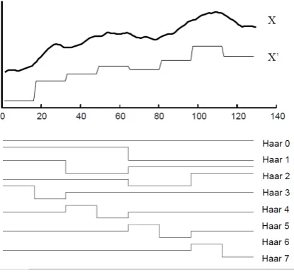
Entire-length.This label refers to methods that apply sim-plification or feature extraction on the entire length of time series and derive a model accordingly. For instance, Discrete Wavelet Transform decomposes the entire signal into a com-bination of Wavelet bases (Fig.3).

Figure 3:The first eight wavelet bases and their linear com-bination X0to represent the original data X . [CF99]

Figure 4: Visual output of the Piecewise Aggregate Approx-imation algorithm [CKMP02]

[KCPM01] is one of the most intuitive and simplistic ap-proaches that produce equi-length segments. The idea be-hind the algorithm is to divide data of lengthnintom equi-sized frames, where 1<m<n. The mean value of the values that fall within boundaries of each frame form the vector of lengthmwhich becomes the reduced representation of the original data. Piecewise Constant Approximation [KP00] al-gorithm is ultimately the same approach towards reduction that has different implications in indexing.

Piecewise Adaptive-length. A more precise representa-tion of the original data is possible if segments of variable length are allowed. However, these approaches may result in approximations that are more difficult to index and query. Adaptive Piecewise Constant Approximation presented in [CKMP02] approximates the time series by segments of constant values with varying lengths (Fig.4). The authors demonstrate that the algorithm provides accurate represen-tation and is indexable, that is, capable of finding neighbors.

6. Detailed Summary

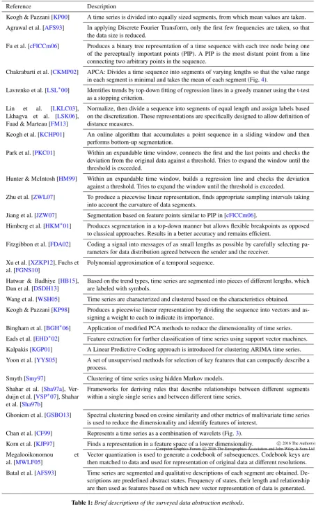
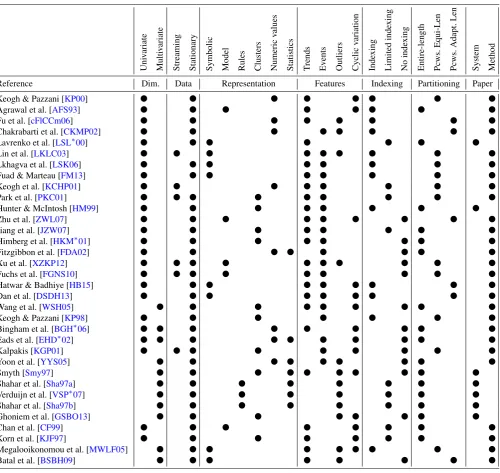
Table1gives a brief overview of the surveyed abstraction methods. Table2summarizes the abstraction methods in re-spect to the properties, which are organized into groups, or facets, according to the classification scheme presented in Section5. This view fulfills several purposes.

1. Allows fast and easy selection of abstraction algo-rithms.

The visualization designer needs to consider the aspects dis-cussed in Section4and then choose an algorithm that satis-fies most or all of the requirements in terms of the data prop-erties, output representation, feature preservation and extrac-tion, and method properties. For example, if the goal is to design an event-driven visualization system with interactive querying capabilities and line chart representation, the visu-alization designer should look for algorithms that satisfy the

Eventsproperty, withSymbolicorReal-valued representa-tion, preferably ofPiecewise-Adaptive Lengthtype and with

Indexingsupport. It may happen that some facets are not im-portant for a particular design and can be ignored. For exam-ple, in case of designing a system for offline analysis, both batch and online algorithms are suitable.

2. Provides examples for classification of new algorithms. The proposed table can be easily extended to include ap-proaches that are not covered in this survey as well as new approaches that continuously appear. A method that is added needs to be evaluated with regard to each group of properties specified in the table header. Note that several properties at once could be satisfied within each facet.

3. Shows principles behind the organization of the prop-erties into groups.

Understanding these principles is a prerequisite for introduc-tion of new meaningful dimensions in the future. We identify two key requirements for including a new group of proper-ties into the framework. First, the properproper-ties in the group must be inclusive, that is, every algorithm must satisfy at least one of the properties in each group. Second, they must be informative. A visualization designer should be able to clearly understand what they lose or gain when they select an abstraction algorithm that satisfies particular properties and fails for others.

7. Future Work

Reference Description

Keogh & Pazzani [KP00] A time series is divided into equally sized segments, from which mean values are taken. Agrawal et al. [AFS93] In applying Discrete Fourier Transform, only the first few frequencies are taken, so that

the data size is reduced.

Fu et al. [cFlCCm06] Produces a binary tree representation of a time sequence with each tree node being one of the perceptually important points (PIP). A PIP is the most distant point from a line connecting two arbitrary points in the sequence.

Chakrabarti et al. [CKMP02] APCA: Divides a time sequence into segments of varying lengths so that the value range in each segment is minimal and takes the mean of each segment (Fig.4).

Lavrenko et al. [LSL∗00] Identifies trends by top-down fitting of regression lines in a greedy manner using the t-test as a stopping criterion.

Lin et al. [LKLC03], Lkhagva et al. [LSK06], Fuad & Marteau [FM13]

Normalize, then divide a sequence into segments of equal length and assign labels based on the discretization. These representations are specifically designed to allow definition of distance measures.

Keogh et al. [KCHP01] An online algorithm that accumulates a point sequence in a sliding window and then performs bottom-up segmentation.

Park et al. [PKC01] Within an expandable time window, connects the first and the last points and checks the deviation from the original data against a threshold. Tries to expand the window until the threshold is exceeded.

Hunter & McIntosh [HM99] Within an expandable time window, builds a regression line and checks the deviation against a threshold. Tries to expand the window until the threshold is exceeded.

Zhu et al. [ZWL07] To produce a piecewise linear representation, finds appropriate sampling intervals taking into account the curvature of data segments.

Jiang et al. [JZW07] Segmentation based on feature points similar to PIP in [cFlCCm06].

Himberg et al. [HKM∗01] Produces segmentation in a top-down manner but allows flexible breakpoints as opposed to classical approaches. Results in a better accuracy and remains efficient.

Fitzgibbon et al. [FDA02] Coding a signal into messages of as small lengths as possible by carefully selecting pa-rameters for data distribution agreed between the sender and the receiver.

Xu et al. [XZKP12], Fuchs et al. [FGNS10]

Polynomial approximation of a temporal sequence. Hatwar & Badhiye [HB15],

Dan et al. [DSDH13]

Based on the trend types, time series are segmented into pieces of different lengths, which are labeled with symbols.

Wang et al. [WSH05] Time series are characterized and clustered based on the characteristics obtained. Keogh & Pazzani [KP98] Produces a piecewise linear representation by dividing the sequence into vectors and

as-signing a weight to each to indicate its importance.

Bingham et al. [BGH∗06] Application of modified PCA methods to reduce the dimensionality of time series. Eads et al. [EHD∗02] Feature extraction for further classification of time series using support vector machines. Kalpakis [KGP01] A Linear Predictive Coding approach is introduced for clustering ARIMA time series. Yoon et al. [YYS05] A set of unsupervised methods for selection of key features that can compactly describe a

process.

Smyth [Smy97] Clustering of time series using hidden Markov models. Shahar et al. [Sha97a],

Ver-duijn et al. [VSP∗07], Shahar et al. [Sha97b]

Frameworks for deriving rules that describe relationships between different segments within a single single series and between different time series.

Ghoniem et al. [GSBO13] Spectral clustering based on cosine similarity and other metrics of multivariate time series is used to reduce the dimensionality and identify features of interest.

Chan et al. [CF99] Represents a time series as a combination of wavelets (Fig.3). Korn et al. [KJF97] Finds a representation in a feature space of a lower dimensionality. Megalooikonomou et

al. [MWLF05]

Vector quantization is used to generate a codebook of subsequences. Codebook keys are then matched to data and used for representation of original data at different resolutions. Batal et al. [AFS93] Time series are segmented and qualitative descriptions of each segment are obtained.

De-scriptions are predefined abstract states. Frequency of states, their length and relationship are then used as features based on which new vector representation of data is generated.

c

Uni

v

ariate

Multi

v

ariate

Streaming Stationary Symbolic Model Rules Clusters Numeric

v

alues

Statistics Trends Ev

ents

Outliers Cyclic

v

ariation

Inde

xing

Limited

inde

xing

No

inde

xing

Entire-length Pcws.

Equi-Len

Pcws.

Adapt.

Len

System Method Reference Dim. Data Representation Features Indexing Partitioning Paper

Keogh & Pazzani [KP00] l l l l l l l l

Agrawal et al. [AFS93] l l l l l l l l

Fu et al. [cFlCCm06] l l l l l l l l

Chakrabarti et al. [CKMP02] l l l l l l l l

Lavrenko et al. [LSL∗00] l l l l l l l

Lin et al. [LKLC03] l l l l l l l l l

Lkhagva et al. [LSK06] l l l l l l l l

Fuad & Marteau [FM13] l l l l l l l l

Keogh et al. [KCHP01] l l l l l l l l

Park et al. [PKC01] l l l l l l l l l

Hunter & McIntosh [HM99] l l l l l l l l

Zhu et al. [ZWL07] l l l l l l l l l

Jiang et al. [JZW07] l l l l l l l l

Himberg et al. [HKM∗01] l l l l l l l l

Fitzgibbon et al. [FDA02] l l l l l l l l

Xu et al. [XZKP12] l l l l l l l l l l

Fuchs et al. [FGNS10] l l l l l l l l l

Hatwar & Badhiye [HB15] l l l l l l l l l

Dan et al. [DSDH13] l l l l l l l l l

Wang et al. [WSH05] l l l l l l l l l

Keogh & Pazzani [KP98] l l l l l l l

Bingham et al. [BGH∗06] l l l l l l l l l

Eads et al. [EHD∗02] l l l l l l l l l l

Kalpakis [KGP01] l l l l l l l l l

Yoon et al. [YYS05] l l l l l l l l l

Smyth [Smy97] l l l l l l l l l l

Shahar et al. [Sha97a] l l l l l l l l

Verduijn et al. [VSP∗07] l l l l l l l l

Shahar et al. [Sha97b] l l l l l l l l

Ghoniem et al. [GSBO13] l l l l l l l l

Chan et al. [CF99] l l l l l l l l

Korn et al. [KJF97] l l l l l l l l

Megalooikonomou et al. [MWLF05] l l l l l l l l l

Batal et al. [BSBH09] l l l l l l l l

7.1. Error Boundaries

Our study of the literature has revealed that a lot effort is being put in deriving quality metrics for data abstractions [BTK11,CWRY06]. It is important to be informed about the degree of abstraction to avoid oversimplification and loss of important features. An error bound guarantee is achieved by assuring that an algorithm will not produce approximations differing from the original data by more than a specified value.

Global error boundary.This is a guarantee that the sum of all errors across the entire length of a time series will not exceed a given value. Piecewise Polynomial Represen-tation [FGNS10] approximates time series segments with polynomials of arbitrary degree. By resorting to the least squares approximation over a sliding/growing time window, the authors achieve an online algorithm with a global error boundary.

Individual error boundary.This is a guarantee that any point in the approximated data will not differ from the corre-sponding point in the original data by more than a specified value. Discrete Fourier Transform [AFS93] was proved to hold the lower bounding condition for its approximation.

No error boundary.In some cases, it turns out to be dif-ficult to provide a proven error boundary although an algo-rithm may perform remarkably well compared to other ap-proaches for which error boundaries have been stated.

One aspect that is often considered as a quality measure is how accurately the model preserves the distances between objects. However, some researchers claim that this measure is not sufficient for temporal data [LP11]. A deeper investi-gation and evaluation of quality measures for temporal data should be carried out.

7.2. Parameters

Algorithms might require some parameterization that strongly affects the output.

Number of segments.Determines the level of accuracy of the output for algorithms involving time series partition-ing. Piecewise Constant Approximation [KP00] proposed by Keogh et al. takeskas the only input to determine the num-ber of equi-sized segments the mean values from which will be taken for the representation.

Resolution. In a case when an algorithm produces a global approximation of time series, the user has to provide, instead of the number of segments, the number of the first coefficients, or the degree of polynomials, or the number of eigenwaves to be used in modeling the original data. This parameter can be referred to as the resolution of the abstrac-tion.

Error bound.This is often an additional parameter, but it may also be the only parameter required by an algorithm.

Approaches that consider the total error bound calculate the sum of residues at all data points. If it exceeds the speci-fied value, the previous approximation is refined so that the the bound is met. Unlike a total error bound, that consid-ers the sum of all errors, an individual error bound is aimed at preserving the distance between each original data point and its approximation at a certain value which must not be exceeded.

Non-parametrized.Some algorithms do not take any pa-rameters and can produce approximation with default set-tings or derive such in an automated manner by heuristics.

As noted by Aigner et al. [AMM∗08a], the user’s ability to tune parameters is an important aspect of the usability of a system or method. At the same time, it is difficult to evaluate how easy or difficult is each approach for different groups of users in different contexts.

7.3. Temporal Characteristics

Aigner et al. [AMM∗08a] emphasize that time should be re-spected as an independent dimension when visualizing tem-poral data; however, the authors admit that even those meth-ods that do not respect time as an independent dimension can be applicable to time series data. An example is Prin-cipal Component Analysis [Jol02], which has been success-fully applied to time series without extracting time as a sep-arate dimension [BDA11]. Hence, even though time should be dealt with in a special way, analytical methods that do not do this may still be capable of producing meaningful re-sults. Consequently, this work could be extended by consid-ering abstraction techniques from the domains of data min-ing other than time series minmin-ing.

8. Conclusion

We have described the challenges of large time series visu-alization and substantiated the need for abstraction. We have discussed the requirements that need to be considered to find a suitable abstraction method for time series visualization.

Our contribution is two-fold. First, we propose a frame-work for the classification of time series abstraction algo-rithms that specifies and justifies the essential criteria for informed method selection. Second, we provide a classifi-cation of a large number of existing abstraction methods, which can be practically used for method selection. It is chal-lenging to make an exhaustive survey of all time series ab-straction methods. However, we believe that the framework we presented, along with the proposed directions for its ex-tension (Section7), provides a good opportunity for obtain-ing a unified picture of data abstraction for large time series and will prove useful for visualization designers, who would be able to either use our model as is or customize/extend it based on their vision.