Cluster-based Vulnerability Assessment of Operating Systems and Web Browsers

City, University of London Institutional Repository

Citation

:

Movahedi, Y., Cukier, M., Andongabo, A. and Gashi, I. ORCID:

0000-0002-8017-3184 (2018). Cluster-based Vulnerability Assessment of Operating Systems and Web

Browsers. Computing, doi: 10.1007/s00607-018-0663-0

This is the published version of the paper.

This version of the publication may differ from the final published

version.

Permanent repository link:

http://openaccess.city.ac.uk/id/eprint/20519/

Link to published version

:

http://dx.doi.org/10.1007/s00607-018-0663-0

Copyright and reuse:

City Research Online aims to make research

outputs of City, University of London available to a wider audience.

Copyright and Moral Rights remain with the author(s) and/or copyright

holders. URLs from City Research Online may be freely distributed and

linked to.

https://doi.org/10.1007/s00607-018-0663-0

Cluster-based vulnerability assessment of operating

systems and web browsers

Yazdan Movahedi1_{·Michel Cukier}1_{·Ambrose Andongabo}2_{·Ilir Gashi}2

Received: 25 September 2017 / Accepted: 15 September 2018 © The Author(s) 2018

Abstract

Organizations face the issue of how to best allocate their security resources. Thus, they need an accurate method for assessing how many new vulnerabilities will be reported for the operating systems (OSs) and web browsers they use in a given time period. Our approach consists of clustering vulnerabilities by leveraging the text information within vulnerability records, and then simulating the mean value function of vulner-abilities by relaxing the monotonic intensity function assumption, which is prevalent among the studies that use software reliability models (SRMs) and nonhomogeneous Poisson process in modeling. We applied our approach to the vulnerabilities of four OSs (Windows, Mac, IOS, and Linux) and four web browsers (Internet Explorer, Safari, Firefox, and Chrome). Out of the total eight OSs and web browsers we analyzed using a power-law model issued from a family of SRMs, the model was statistically adequate for modeling in six cases. For these cases, in terms of estimation and fore-casting capability, our results, compared to a power-law model without clustering, are more accurate in all cases but one.

Keywords Vulnerability assessment·Nonhomogeneous Poisson process· Clustering·Software reliability models·Software reliability growth·Security growth models

Mathematics Subject Classification 62H30·68M15

B

[email protected]

Yazdan Movahedi [email protected]

Michel Cukier [email protected]

Ambrose Andongabo

[email protected]

1 _{University of Maryland, College Park, USA}

1 Introduction

Security decision makers often use public data sources to help make better decisions on, for example, selecting security products, checking for security trends, and estimat-ing when new vulnerabilities that affect their installations will be publicly reported. Several studies have applied software reliability models (SRMs) to estimate times between public reports of vulnerabilities [1–6]. The studies we are aware of estimate all vulnerabilities together. We postulate that such analysis may miss some insights that apply to separate categories of vulnerabilities, rather than all vulnerabilities together. Moreover, SRMs assume vulnerability detection to be an independent process. How-ever, this might not be the case due, for example, to the discovery of a new type of vulnerability that might prompt attackers to look for similar vulnerabilities [7]. This may lead to less accurate predictions on the next reporting date of vulnerability, or the total number of new vulnerabilities reported in the next time interval. One way to mitigate these issues is to split vulnerabilities into separate clusters and test whether the clusters are independent.

In this paper we present an approach that does the following:

– Uses existing clustering techniques to group vulnerabilities into distinct clusters, using the textual information reported in the vulnerabilities as a basis for con-structing the clusters;

– Uses existing SRMs to make predictions on the number of new vulnerabilities that will be discovered in a given time period for each cluster for a given OS/web browser;

– Superposes the SRMs used for each cluster together into a single model for pre-dicting the number of vulnerabilities that will be discovered in a given time period for a given OS/web browser.

We have applied our approach on vulnerabilities of four different OSs (Windows (Microsoft), Mac (Apple), IOS (Cisco) and Linux) and four web browsers [Internet Explorer (Microsoft), Safari (Apple), Firefox (Mozilla), and Chrome (Google)]. For these OSs, our approach when compared to a power-law model without clustering issued from a family of SRMs, gives more accurate curve fittings and predictions in all cases we analyzed. For these web browsers, in all the cases where the power-law model is statistically adequate for modeling (at least one of the models has apvalue greater than 0.05), our approach provides more accurate or more conservative curve fitting and forecasting results.

The rest of the paper is structured as follows. Section2presents the related work. Section3 details the dataset and how we processed the data. Section 4details the analysis. Section5presents the obtained results. Section6discusses the results and lists the limitations. Finally, Sect.7concludes the paper.

2 Related work

(SRMs) can be considered similar based on the fault detection processes. Thus, the intensity function can represent the detection rate of vulnerabilities [8]. Research has been conducted to create a link between the fault discovery process and the vulner-ability discovery process for modeling purposes [9]. Several studies have proposed new SRMs/ VDMs or applied existing models to estimate software security indicators such as total number of residual vulnerabilities in the system, time to next vulnerability (TTNV), vulnerability detection rate [1–4,7–13].

Rescorla [2,3] proposed a VDM to find the number of undiscovered vulnerabilities. In [4–6], Alhazmi and Malaiya proposed regression models to simulate the vulner-ability disclosure rate and predict the number of vulnerabilities that may be present but may not yet have been found. Some studies have tried to increase the accuracy of vulnerability modeling. Joh and Malaiya [14] proposed a new approach for modeling the skewness in vulnerability datasets by modifying common S-shaped models like Weibull and Gamma. These models assume that the software under study has a finite number of vulnerabilities to be discovered [8]. Note that, releasing new patches might be accompanied by introducing new vulnerabilities and dynamically change the num-ber of vulnerabilities. The mentioned models provide better curve fitting results than prediction ones. This is because a model may provide an excellent fit for the available data points, but if the detection trends are not consistent with the model, the model doesn’t lead to accurate prediction results [14].

In addition to the vulnerabilities publication dates, software source code has been used for vulnerability assessment in the context of VDMs. Kim et al. [15] introduced a VDM based on shared source code measurements among multi-version software systems. In [16], Ozment and Schechter employed a reliability growth model to analyze the security of the OpenBSD OS by examining its source code and the rate at which new code has been introduced. However, source code has proved not to be an accurate measure in terms of prediction [7].

Clustering is a method of structuring data according to similarities and dissimi-larities into natural groupings [17]. Clustering for vulnerabilities has been used for splitting real-world exploited vulnerabilities from those which were exploited during software test (proof-of-concept exploits) [18], as well as for detecting exploited vul-nerabilities versus non-exploited ones when there is not enough information about some vulnerabilities [19]. Lee et al. [20] investigated a distributed denial of service (DDoS) attack detection method using cluster analysis. Shahzad et al. [21] conducted a descriptive statistical analysis of a large software vulnerability dataset employing clustering on type-based vulnerability data. Huang et al. [22] classified vulnerabilities employing several clustering algorithms to create a relatively objective classification criterion among the vulnerabilities.

3 Dataset and data processing

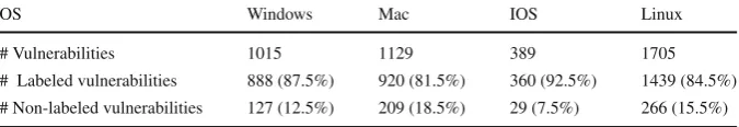
Table 1 Number of vulnerabilities per OS

OS Windows Mac IOS Linux

# Vulnerabilities 1015 1129 389 1705

# Labeled vulnerabilities 888 (87.5%) 920 (81.5%) 360 (92.5%) 1439 (84.5%)

# Non-labeled vulnerabilities 127 (12.5%) 209 (18.5%) 29 (7.5%) 266 (15.5%)

identifier. We used the CVE ID to compare the reporting date of each vulnerability in NVD, with the dates in other public repositories on vulnerabilities.1We then updated the reporting date on our database to the earliest date that a given vulnerability was known in any of these databases. Details of the tool (vepRisk) we developed to gather the data is given in [23]. For the rest of the paper, we will focus on four OSs (Windows, Mac, IOS, and Linux) and four web browsers (Internet Explorer, Safari, Firefox, and Chrome).

3.1 Operating systems

We will focus on the vulnerabilities reported for four well-known OSs: Windows (1995–2016), Mac (1997–2016), IOS (the OS associated with Cisco) (1992–2016), and Linux (1994–2016). We chose these OSs as they are most widely used, and had the most vulnerabilities in NVD. For each OS, we included all the vulnerabilities reported for any of its versions. For instance, all the vulnerabilities reported for mac-os, mac-os-server, mac-os-x, and mac-os-x-server were put together to create a dataset for Mac. We did this to have enough data for each OS. The total number of vulnerabilities in NVD for these OSs is 4238. We used text information within vulnerabilities reports to then label the vulnerabilities. The keywords for labeling (e.g., denial, injection, buffer, execute) were extracted from these reports. Table1 shows the total number of vulnerabilities as well as the number of labeled and non-labeled (vulnerabilities without any associated text information in the database) vulnerabilities for these OSs. For the labeled vulnerabilities, we indicate the number and proportion of vulner-abilities associated with a specific keyword. Note that vulnervulner-abilities can be labeled with more than one keyword. Details for OSs are in Table2.

We treated each keyword as a binary variable. Thus, each vulnerability is repre-sented as a matrix with a binary vector; if a keyword is present in the textual information of a given vulnerability, the value of that keyword is “1” otherwise, the values is “0”. We excluded non-labeled vulnerabilities from our clusters. For cluster analysis, we need to ensure that the features (keywords) are not correlated. Therefore, we checked the Pearson correlation coefficient for every two keywords per OS. When we found statistically significant correlation, we merged the correlated keywords with a title which included both terms. For instance, due to the high correlation of 0.99 (pvalue < 0.001,H0 :p=0) between “Execute” and “Code” for all OSs, these terms were treated as “Execute Code”. The same applied for the keywords “SQL” and “Injec-tion”. No other significant correlation was observed.

Table 2 Number of vulnerabilities per type and OS

Keywords Windows Mac IOS Linux

Denial of service 242 (27.25%) 412 (44.8%) 296 (82.2%) 860 (59.8%)

Execute code 289 (32.5%) 458 (49.8%) 24 (6.7%) 161 (11.2%)

Overflow 174 (19.6%) 338 (36.7%) 29 (8.1%) 298 (20.7%)

SQL injection 0 0 0 4 (0.3%)

Obtain information 49 (5.5%) 113 (12.3%) 9 (2.5%) 229 (15.9%)

Gain privileges 325 (36.6%) 116 (12.6%) 4 (1.1%) 205 (14.25%) Bypass restriction or similar 62 (7.0%) 115 (12.5%) 38 (10.6%) 112 (7.8%)

Directory traversal 2 (0.2%) 12 (1.3%) 4 (1.1%) 8 (0.6%)

Cross site scripting 10 (1.1%) 15 (1.6%) 2 (0.6%) 11 (0.8%)

Http response splitting 0 2 (0.2%) 0 1 (0.07%)

CSRF 0 2 (0.2%) 1 (0.3%) 0

Memory corruption 59 (6.6%) 145 (15.8%) 5 (1.4%) 70 (4.9%)

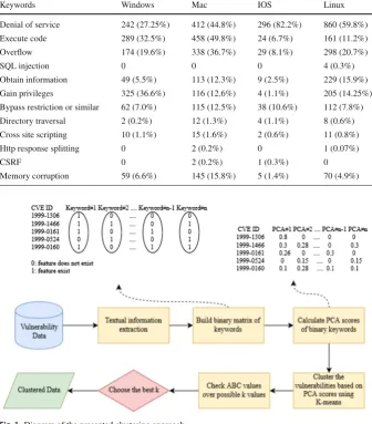
Fig. 1 Diagram of the presented clustering approach

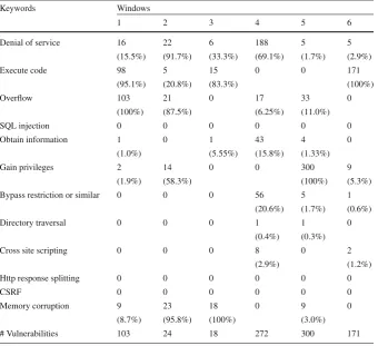
Table 3 Number of vulnerabilities per type, cluster (Windows)

Keywords Windows

1 2 3 4 5 6

Denial of service 16 22 6 188 5 5

(15.5%) (91.7%) (33.3%) (69.1%) (1.7%) (2.9%)

Execute code 98 5 15 0 0 171

(95.1%) (20.8%) (83.3%) (100%)

Overflow 103 21 0 17 33 0

(100%) (87.5%) (6.25%) (11.0%)

SQL injection 0 0 0 0 0 0

Obtain information 1 0 1 43 4 0

(1.0%) (5.55%) (15.8%) (1.33%)

Gain privileges 2 14 0 0 300 9

(1.9%) (58.3%) (100%) (5.3%)

Bypass restriction or similar 0 0 0 56 5 1

(20.6%) (1.7%) (0.6%)

Directory traversal 0 0 0 1 1 0

(0.4%) (0.3%)

Cross site scripting 0 0 0 8 0 2

(2.9%) (1.2%)

Http response splitting 0 0 0 0 0 0

CSRF 0 0 0 0 0 0

Memory corruption 9 23 18 0 9 0

(8.7%) (95.8%) (100%) (3.0%)

# Vulnerabilities 103 24 18 272 300 171

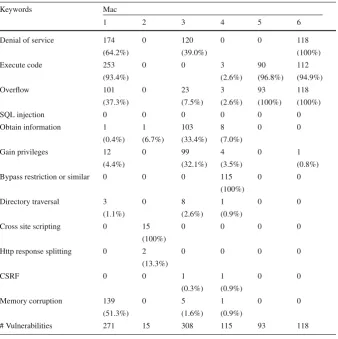
Table 4 Number of vulnerabilities per type, cluster (Mac)

Keywords Mac

1 2 3 4 5 6

Denial of service 174 0 120 0 0 118

(64.2%) (39.0%) (100%)

Execute code 253 0 0 3 90 112

(93.4%) (2.6%) (96.8%) (94.9%)

Overflow 101 0 23 3 93 118

(37.3%) (7.5%) (2.6%) (100%) (100%)

SQL injection 0 0 0 0 0 0

Obtain information 1 1 103 8 0 0

(0.4%) (6.7%) (33.4%) (7.0%)

Gain privileges 12 0 99 4 0 1

(4.4%) (32.1%) (3.5%) (0.8%)

Bypass restriction or similar 0 0 0 115 0 0

(100%)

Directory traversal 3 0 8 1 0 0

(1.1%) (2.6%) (0.9%)

Cross site scripting 0 15 0 0 0 0

(100%)

Http response splitting 0 2 0 0 0 0

(13.3%)

CSRF 0 0 1 1 0 0

(0.3%) (0.9%)

Memory corruption 139 0 5 1 0 0

(51.3%) (1.6%) (0.9%)

# Vulnerabilities 271 15 308 115 93 118

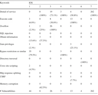
We assumed that the keywords which covered at least 60% of vulnerabilities in each cluster can be good representatives of relative clusters. Since none of the keywords reached the weight threshold of 0.6 in the third cluster associated with Mac, the keyword with the greatest weight (Denial of Service) was selected as the cluster’s label. There is only one common cluster name among all the OSs. There are also clusters with similar names within some OSs.

However, analyzing their linear correlation, we did not find any significant rela-tionship based on the Pearson correlation test. Table7shows the cluster summaries for the OSs.

3.2 Web browsers

Table 5 Number of vulnerabilities per type, cluster (IOS)

Keywords IOS

1 2 3 4 5 6 7

Denial of service 0 8 19 3 4 0 262

(100%) (73.1%) (100%) (30.8%) (100%)

Execute code 3 0 8 0 13 0 0

(6.8%) (30.8%) (100%)

Overflow 1 2 26 0 0 0 0

(2.3%) (25%) (100%)

SQL injection 0 0 0 0 0 0 0

Obtain information 6 3 0 0 0 0 0

(13.6%) (37.5%)

Gain privileges 1 0 0 0 3 0 0

(2.3%) (23.1%)

Bypass restriction or similar 35 0 0 3 0 0 0

(79.5%) (100%)

Directory traversal 0 0 0 0 0 4 0

(100%)

Cross site scripting 2 0 0 0 0 0 0

(4.5%)

Http response splitting 0 0 0 0 0 0 0

CSRF 0 0 0 0 1 0 0

(7.7%)

Memory corruption 0 5 0 0 0 0 0

(62.5%)

# Vulnerabilities 44 8 26 3 13 4 262

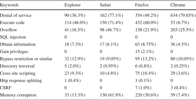
(2008–2016). These browsers were selected since they are widely used and had the highest number of vulnerabilities in the database. Similar to what we did for OSs, we considered, for each browser, all the vulnerabilities reported for any of its versions. As an example, all the vulnerabilities reported for ie, ieexplorer, and ie-for-macintosh were combined under Internet Explorer. Thus, we had enough data for each browser. The total number of vulnerabilities for these browsers is 2434. The process of extract-ing text information from vulnerability reports and labelextract-ing vulnerabilities is the same as for the OSs. The total number of vulnerabilities as well as the number of labeled and non-labeled vulnerabilities for the selected browsers are presented in Table 8. Table9shows the number and proportion of vulnerabilities associated with a specific keyword for the labeled vulnerabilities. As previously mentioned, vulnerabilities can be labeled with more than one keyword.

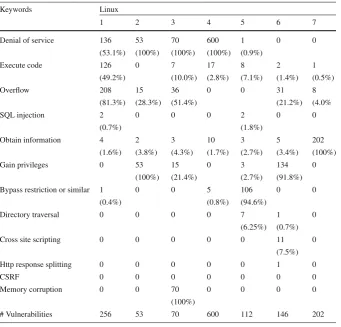
Table 6 Number of vulnerabilities per type, cluster (Linux)

Keywords Linux

1 2 3 4 5 6 7

Denial of service 136 53 70 600 1 0 0

(53.1%) (100%) (100%) (100%) (0.9%)

Execute code 126 0 7 17 8 2 1

(49.2%) (10.0%) (2.8%) (7.1%) (1.4%) (0.5%)

Overflow 208 15 36 0 0 31 8

(81.3%) (28.3%) (51.4%) (21.2%) (4.0%

SQL injection 2 0 0 0 2 0 0

(0.7%) (1.8%)

Obtain information 4 2 3 10 3 5 202

(1.6%) (3.8%) (4.3%) (1.7%) (2.7%) (3.4%) (100%)

Gain privileges 0 53 15 0 3 134 0

(100%) (21.4%) (2.7%) (91.8%)

Bypass restriction or similar 1 0 0 5 106 0 0

(0.4%) (0.8%) (94.6%)

Directory traversal 0 0 0 0 7 1 0

(6.25%) (0.7%)

Cross site scripting 0 0 0 0 0 11 0

(7.5%)

Http response splitting 0 0 0 0 0 1 0

CSRF 0 0 0 0 0 0 0

Memory corruption 0 0 70 0 0 0 0

(100%)

# Vulnerabilities 256 53 70 600 112 146 202

that the keywords which covered at least 60% of vulnerabilities in each cluster can be good representatives of relative clusters. For those clusters, for which none of the keywords reach the weight threshold (i.e., cluster #2 in Safari), the keyword with the greatest weight becomes the cluster’s label. The cluster summaries for the browsers are shown in Table10. More details about the clusters and frequency of the keywords associated with the clusters are provided in the following report online2(we had to remove them from the paper due to space constraints).

4 Analysis

A nonhomogeneous Poisson process (NHPP) is often used when modeling the mean cumulative number of failures (MCF) for repairable systems and for software reliabil-ity evaluations. The core assumption is that the number of detected failures follows a

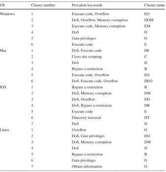
Table 7 Cluster composition for operating systems

OS Cluster number Prevalent keywords Cluster name

Windows 1 Execute code, Overflow EO

2 DoS, Overflow, Memory corruption DOM

3 Execute code, Memory corruption EM

4 DoS D

5 Gain privileges G

6 Execute code E

Mac 1 DoS, Execute code DE

2 Cross site scripting C

3 DoS D

4 Bypass a restriction B

5 Execute code, Overflow EO

6 DoS, Execute code, Overflow DEO

IOS 1 Bypass a restriction B

2 DoS, Memory corruption DM

3 DoS, Overflow DO

4 DoS, Bypass a restriction DB

5 Execute code E

6 Directory traversal DT

7 DoS D

Linux 1 Overflow O

2 DoS, Gain privileges DG

3 DoS, Memory corruption DM

4 DoS D

5 Bypass a restriction B

6 Gain privileges G

7 Obtain information O

Table 8 Number of vulnerabilities per web browser

Web browser Explorer Safari Firefox Chrome

# Vulnerabilities 379 248 890 917

# Labeled vulnerabilities 248 (65.4%) 210 (84.7%) 720 (80.8%) 796 (86.8%) # Non-labeled vulnerabilities 131 (34.6%) 38 (15.3%) 170 (19.2%) 121 (13.2%)

nonhomogeneous Poisson process. In the case of NHPP-based repairable systems, the intensity functionλ(t)=d E[Λ(t)]/dtis often assumed to be a monotonic function of t. Similarly, in NHPP-based software reliability models (SRMs), the intensity function (the detection rate of software errors) is considered to be a monotonic function [28].

Table 9 Number of vulnerabilities per type and web browser

Keywords Explorer Safari Firefox Chrome

Denial of service 90 (36.3%) 162 (77.1%) 354 (49.2%) 634 (79.65%)

Execute code 114 (46.0%) 150 (71.4%) 432 (60.0%) 53 (6.7%)

Overflow 41 (16.5%) 98 (46.7%) 158 (21.9%) 203 (25.5%)

SQL injection 0 0 0 0

Obtain information 18 (7.3%) 17 (8.1%) 63 (8.75%) 36 (4.5%)

Gain privileges 0 0 15 (2.1%) 0

Bypass restriction or similar 32 (12.9%) 19 (9.05%) 95 (13.2%) 80 (10.05%)

Directory traversal 5 (2.0%) 2 (0.95%) 6 (0.8%) 2 (0.25%)

Cross site scripting 23 (9.3%) 10 (4.8%) 75 (10.4%) 29 (3.6%)

Http response splitting 1 (0.4%) 0 1 (0.1%) 0

CSRF 0 0 7 (1.0%) 3 (0.4%)

Memory corruption 33 (13.3%) 130 (61.9%) 220 (30.6%) 59 (7.4%)

Table 10 Cluster composition for web browsers

Web browser Cluster number Prevalent keywords Cluster name

Internet Explorer 1 DoS D

2 Execute code, Memory corruption, DoS EMD

3 Bypass a restriction B

4 Execute code E

5 Cross Site Scripting C

Safari 1 Execute code, Memory corruption, DoS EMD

2 DoS (0.29), Bypass a restriction (0.29) DB

3 Execute code, Memory corruption, DoS, Overflow EMDO

Firefox 1 Execute code, Overflow EO

2 Execute code, Memory corruption, DoS EMD

3 Bypass a restriction (0.34) B

4 Execute code, Memory corruption, DoS, Overflow EMDO

5 Execute code E

Chrome 1 Bypass a restriction B

2 Memory corruption, DoS, Overflow MDO

3 Memory corruption, DoS MD

4 DoS, Overflow DO

5 DoS D

to be compromised, then the superposition model represents the software failures. Let us assume that we are dealing with vulnerabilities classified into independent clusters. LetΛj(t)denote the NHPP for the vulnerabilities from the jth cluster in

(0 t] with intensity functionλj(t|αj, βj)where the function form ofλj(t|αj, βj)is

number of vulnerabilities from any jth clusterΛj(t),j =1,2. . .J is independent.

A processΛ(t)=J_j=1Λj(t),which counts the total number of vulnerabilities in

the interval (0 t] for the superposition model, is also a non-homogeneous Poisson process with an intensity functionλ(t|α, β) = λ1(t|α1, β1)+ · · · +λ1(t|αJ, βJ),

whereα= {α1, . . . , αJ},β = {β1, . . . , βJ}. Since the superposition model remains

an NHPP (all intensity functions are NHPPs), the associated superposition model can be applicable [28]. Two important cases of NHPPs consist of the related intensity function following a power-law and log linear (exponential) function of time [29,30]. In such case, the equations become:

λj(t|αj, βj)= αj

βj

t

βj _αj−1

=αjtαj−1

βαj

j

(1)

Λ(t)= t

0 J

j=1

λj(t|αj, βj)dt, αj >0, βj >0 (2)

In this paper, we expect to obtain better assessment results when relaxing the mono-tonicity assumption of the intensity function that is prevalent in SRMs and VDMs. We created independent clusters that can be modeled using separate NHPPs. In this paper, we selected the power-law model since Allodi [31] showed that vulnerabilities may follow a power-law distribution. In addition, the power-law model has been widely used in research on software reliability analysis [32–34]. We considered two models for this paper. The first model is a NHPP-based SRM, which uses non-clustered data (including all the labeled and non-labeled vulnerabilities). The second model is the superposition of the NHPPs fitted to the clustered data (only the labeled vulnerabilities can be used to create the clusters), which relaxes the monotonicity assumption of the intensity function. The purpose of both models is to fit and predict the total number of reported vulnerabilities (labeled and non-labeled).

The analysis was done in two steps. First, we used the time difference between vulnerability report dates to find the model parameters from the process of fitting NHPPs to the data (clustered and non-clustered). The models were fitted to the datasets using a non-linear regression method described in [35] that uses a minimiza-tion algorithm called “Levenber g−Mar quar dt” to estimate the parameter values. Non-homogeneity of the clusters were also validated by looking at Laplace-trend test results provided by MiniTab 16 to see whether there were meaningful trends in the clusters. Second, we used the estimated parameters and the models, and simulated corresponding MCFs (one MCF for clustered data, and one for non-clustered data) starting fromt0=0 and time interval of 30 days.

5 Results

the data). We first discuss the results obtained for the four OSs and then for the four web browsers.

5.1 Operating systems

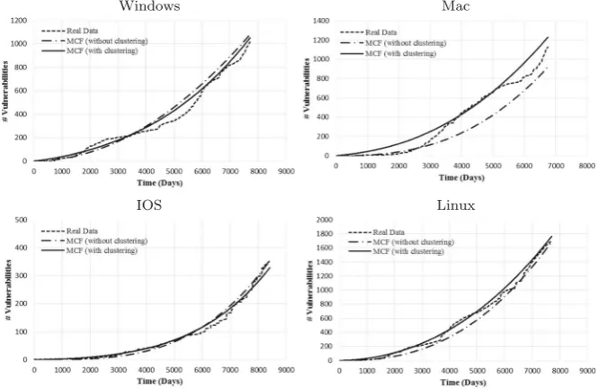
Figure2shows the observed vulnerability data, the MCF obtained without clustering the data and the superimposed MCF when clustering is applied for the four OSs. For Windows, the MCF with clustering is more conservative during roughly the first 3000 days then the MCF without clustering becomes more conservative. The real data crosses the estimates between roughly 2000 and 3000 days. Besides this period, the MCF with and without clustering provide more conservative estimates. For IOS, the MCF with and without clustering as well as the real data are almost overlapping. For Mac and Linux, the MCF with clustering is above the MCF without clustering, providing a more conservative estimation. The real data is above the MCF without clustering and for a short period above the MCF with clustering. Thus for Mac and Linux, the MCF with clustering provide more conservative and accurate estimates.

The analysis of forecasting is done for the final third of the time period from the beginning of the vulnerability discovery process. During the training period (first two thirds of the time period), all the available data are used to estimate model parameters. Figure 3 shows the forecast of the number of vulnerabilities based on the MCFs calculated with and without clustering compared to the observed vulnerabilities. For the vulnerabilities associated with Windows, the forecast with clustering leads to more conservative and more accurate estimates compared to non-clustering. In addition, the forecast without clustering remains below the observed vulnerability data (real data) for the prediction time period which started after day 5088. Both models lead to more conservative predictions for the vulnerabilities associated with Mac. However, the clustering-based MCF trajectory provides more accurate predictions. For IOS the forecast without clustering is more conservative compared to the forecast with clustering. When the MCF without clustering remains above the real data (which is good), it is not the case of the forecast with clustering where the real data crosses the forecast after day 7500. For Linux, the predictions with clustering and the real observed data are close but the forecast remains above the real data and thus provides conservative estimation (which is good). The clustering-based MCF is, however, more accurate than that of the non-clustering MCF.

We applied the Chi-square (χ2_{) goodness of fit test [14] to see how well each} model fits the datasets for both estimation and forecasting. The Chi-square statistic is calculated using the following equation:

χ2₌ N

i=1

(Si −Oi)2

Oi (3)

Windows Mac

IOS Linux

Fig. 2 Comparison of clustered and non-clustered MCFs with vulnerability data

Windows Mac

IOS Linux

Fig. 3 Comparison of clustered and non-clustered forecasts with vulnerability data

R2is another fitting statistic widely used in regression analysis [17,36].R2values close to 1 indicates a good fit. We also considered an additional error indicator to compare the accuracy of the results derived from both models. The normalized root mean square error (NRMSE) is often used. However, Mentaschi et al. [37] showed that for some applications (e.g., high fluctuation of real data) the higher values of NRMSE are not always a reliable indicator of the accuracy of simulations. To remedy the situation, a corrected estimator HH was proposed by Hanna and Heinold [38]:

H H =

N

i=1(Si−Oi)2 N

i=1SiOi

(4)

where Si is theith simulated data,Oi is theith observation and N is the number of observations (the time blocks used for simulation). The closer to zero HH is, the more accurate the model.

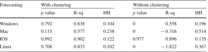
Table11contains the Chi-square goodness of fit test for the clustering-based MCF and the MCF without clustering, the values of R2, and HH for the vulnerabilities of the four OSs in our study. We considered the entire dataset for analyzing estimation accuracy. When considering the entire dataset, both estimations (with/without clus-tering) are statistically sound for all OSs but one (Mac, without clusclus-tering) with p

values greater than 0.05. The Chi-square test results indicate that both fits are reason-ably good in most cases except the case associated with the non-clustered based MCF on Mac data. The R2statistics show that estimations based on clustering are more accurate than the ones without clustering. HH results also show that clustering based estimations came up with smaller errors compared with non-clustering. For the four OSs, the estimations based on clustering were more accurate in all cases. In addition, the MCF model without clustering was not statistically adequate to model the vulner-ability data in one case (Mac). Table12contains the Chi-square goodness of fit test for prediction values of the clustering and non-clustering-based MCF, theR2and HH prediction values for the vulnerabilities of the four OSs. We considered the common 66% splits between training and forecasting which means all the available data in the first two thirds of the study time period were used to estimate model parameters.

Table 11 Estimation accuracy for the four operating systems

Estimation With clustering Without clustering

pvalue R-sq HH pvalue R-sq HH

Windows 1 0.975 0.098 1 0.945 0.145

Mac 0.052 0.851 0.242 0.028 0.837 0.326

IOS 1 0.987 0.084 1 0.972 0.098

Linux 1 0.995 0.06 1 0.992 0.099

Table 12 Forecasting accuracy for the four operating systems

Forecasting With clustering Without clustering

pvalue R-sq HH pvalue R-sq HH

Windows 0.792 0.838 0.104 0 0.558 0.196

Mac 0.115 0.577 0.238 0 −0.316 0.514

IOS 0.992 0.902 0.122 0.977 0.896 0.135

Linux 0.708 0.833 0.102 0 −1.822 0.367

5.2 Web browsers

Figure4shows the observed vulnerability data, the MCF obtained without clustering the data and the superimposed MCF when clustering is applied for the four web browsers. For Internet Explorer, the observed number of vulnerabilities almost leveled off after 4000 days which means the relative vulnerability detection rate decreased. Both MCFs with and without clustering seem inadequate in modeling Internet Explorer data since they are power-law based equations and are designed to model data with constant or increasing discovery rate. Thus, both MCFs show high deviations from the real data. The number of vulnerabilities associated with Chrome also experiences a similar condition after day 1500, and both MCFs seem inappropriate for modeling such S-shaped data. However, in the first 1500 days the MCF with clustering is more conservative than the MCF without clustering. For Safari, despite large fluctuation at day 3400, both MCFs are capable of providing good fits to the real data. However, the MCF with clustering seems to be closer to the observed data, most of the time, but is less conservative. For Firefox, which has almost constant discovery rate, the MCF with clustering is more accurate and more conservative than the MCF without clustering, especially after day 1500. In summary, the MCF with clustering provides more accurate estimations for Safari and Firefox. However, for Internet Explorer and Chrome, the power-law model is not adequate for curve-fitting purposes.

Explorer Safari

Firefox Chrome

Fig. 4 Comparison of clustered and non-clustered MCFs with vulnerability data

For the vulnerabilities associated with Internet Explorer and Chrome, similar to what we observed for estimation, both MCFs forecasting results are distant from the real data. Since both MCFs (with/without clustering) for Internet Explorer and Chrome highly deviate from the real data, we observe that the power-law model is not suitable for modeling this data. For Safari, the forecast with clustering provides more accurate predictions compared to the forecast without clustering. The MCF without clustering was unable to provide accurate forecasts after day 3300. For Firefox, both MCFs provide very accurate forecasts until day 3530. Starting from day 3530, both MCFs provide conservative but less accurate forecasts, (the MCF with clustering provides slightly conservative results).

Table13contains the Chi-square goodness of fit test for the clustering-based MCF and the MCF without clustering, the values ofR2, and HH for the vulnerabilities of the four web browsers. When analyzing estimation accuracy, both MCFs (with/without clustering) are statistically significant for two browsers (Safari and Firefox) with p

values greater than 0.05. The Chi-square test results indicate that both MCFs are not statistically significant for Internet Explorer and Chrome which means that the selected power-law model is not suitable for modeling the data with such attributes (i.e., data with decreasing discovery rate in their overall discovery trend). TheR2statistics/values for Safari and Firefox are almost equal per case, and indicate that both models have provided good fit to the real data. The HH results show that clustering based estimations have smaller errors compared with non-clustering for Safari and Firefox.

Explorer Safari

Firefox Chrome

Fig. 5 Comparison of clustered and non-clustered forecasts with vulnerability data

Table 13 Estimation accuracy

for the four Web Browsers Estimation With clustering Without clustering pvalue R-sq HH pvalue R-sq HH

Explorer 0 0.92 0.31 0 0.95 0.21

Safari 0.96 0.98 0.12 0.90 0.97 0.13

Firefox 1 0.99 0.084 0.98 0.99 0.15

Chrome 0 0.88 0.455 0 0.88 0.295

Table 14 Forecasting accuracy for the four Web Browsers

Forecasting With clustering Without clustering

pvalue R-sq HH pvalue R-sq HH

Explorer 0 0.89 0.16 0 0.89 0.39

Safari 1 0.94 0.11 0 0.90 0.54

Firefox 0.98 0.98 0.071 0.98 0.98 0.057

Chrome 0 0.94 0.51 0 0.94 0.315

For the vulnerabilities associated with Internet Explorer and Chrome, all considered forecasting results using both clustered/non-clustered data lead topvalues less than 0.5. However, it will not be a problem since due to high fluctuation of vulnerability data, HH values are recommended to compare the modeling strategies in terms of prediction. Almost all the research in this area used normalized predictability metrics like HH, NRMSE, and average error (AE) for making predictability comparisons between SRMs/VDMs.

the MCF with clustering is also smaller than that without clustering. For Firefox, both models lead to statistically significant results. The forecasts are very close based on the R-squared values. However, the HH values show that the model without clustering provides more accurate results than the model with clustering.

6 Limitations

The main limitation of the work we present in the paper is with regard to using SRMs as VDMs. Software reliability models usually assume that the time between failures represents total usage time of that product. What we are using is calendar time, which may not be a good proxy for usage. Crucially the difference in security is the difficulty in estimating the “attacker effort”—the total amount of time that an attacker spends in finding a vulnerability—which is something that is not needed for reliability (we assume the users accidentally encounter faults that lead to failures, hence usage time is a good enough proxy for time between failures). A useful discussion of this is given in [39]. Note that this limitation is not only for our work, but applies to research that uses SRMs as VDM and utilizes vulnerability data. However, attacker effort is something that is very difficult to estimate and quantify. The purpose of our research is hence to make as good a use as possible of the publicly available security data to help with decision making. But at the same time to be clear about the limitations on what we can conclude from this analysis. The best we can say from the analysis we present is “the total number of vulnerabilities that will be reported in the NVD over an interval t for product x is y with confidence z”. And we show that we can do this prediction better with clustering than without clustering for four of the largest and most commonly used operating system and web browsers families. For some decision makers this may be a valuable piece of additional information, which they can use in conjunction with data they have from their own installations, when deciding on security operating system/web browser/product choices, and provisioning of security support services to deal with new vulnerabilities.

We have only applied the approach to four well-known operating systems and web browsers that had the largest number of vulnerabilities compared to others. We do not know yet how well this works for other operating systems and web browsers or other applications like databases, though we plan to extend this work in the future.

7 Conclusions

We provided results from applying our approach to vulnerabilities of four different OSs (Windows, Mac, IOS, and Linux) and four web browsers (Internet Explorer, Safari, Firefox, and Chrome), and comparisons of the predictive accuracy of our approach compared with an NHPP model (with monotonic intensity function) that does not use clustering. For the OSs, we found that our approach with clustering, compared with the same modeling mechanism without clustering:

– Is statistically adequate in terms of model fitting and forecasting based upon the Chi-squared goodness of fit test results for all cases we analyzed, while the model without clustering was not statistically sound in 4 out of 8 cases analyzed – Gives more conservative forecasting results in all cases while the model without

clustering was not conservative for Windows

– Gives more accurate results for all the cases analyzed compared to non-clustering. For the web browsers, we found that our approach with clustering, compared with the same modeling mechanism without clustering:

– Gives more accurate results in terms of curve-fitting for all cases where the power-law model was statistically sound to model the data (i.e., Safari and Firefox) – Leads to statistically insignificant results in terms of prediction for two browsers

with or without clustering . For Firefox, the forecasting results are less accurate but slightly more conservative for non-clustering compared to clustering. These results look encouraging, especially as they have been applied for some of the most widely used software products (operating systems and web browsers) which tend to have the highest number of vulnerabilities reported.

Acknowledgements This research is supported by NSF Award #1223634, and the UK EPSRC project D3S (Diversity and defence in depth for security: a probabilistic approach) and the European Commission through the H2020 programme under Grant Agreement 700692 (DiSIEM).

Open Access This article is distributed under the terms of the Creative Commons Attribution 4.0 Interna-tional License (http://creativecommons.org/licenses/by/4.0/), which permits unrestricted use, distribution, and reproduction in any medium, provided you give appropriate credit to the original author(s) and the source, provide a link to the Creative Commons license, and indicate if changes were made.

References

1. Lyu MR (ed) (1996) Handbook of software reliability engineering. IEEE Computer Society Press, Los Alamitos; McGraw Hill, New York

2. Rescorla E (2003) Security holes... Who cares? In: Proceedings of the 12th conference on USENIX Security Symposium, pp 75–90

3. Rescorla E (2005) Is finding security holes a good idea? IEEE Secur Priv Mag 3:14–19

4. Alhazmi O, Malaiya Y (2005) Quantitative vulnerability assessment of systems software. IEEE, pp 615–620

5. Woo S, Alhazmi O, Malaiya Y (2006) Assessing Vulnerabilities in Apache and IIS HTTP Servers. IEEE, pp 103–110

6. Alhazmi O, Malaiya Y (2008) Application of vulnerability discovery models to major operating sys-tems. IEEE Trans Reliab 57:14–22

9. Verissimo P, Neves N, Cachin C, Poritz J, Powell D, Deswarte Y, Stroud R, Welch I (2006) Intrusion-tolerant middleware: the road to automatic security. IEEE Secur Priv Mag 4:54–62

10. Okamura H, Tokuzane M, Dohi T (2013) Quantitative security evaluation for software system from vulnerability database. J Softw Eng Appl 06:15

11. Arbaugh WA, Fithen WL, McHugh J (2000) Windows of vulnerability: a case study analysis. Computer 33:52–59

12. Frei S, May M, Fiedler U, Plattner B (2006) Large-scale vulnerability analysis. In: Proceedings of the 2006 SIGCOMM workshop on large-scale attack defense, LSAD ’06, New York, NY, USA. ACM, pp 131–138

13. Frei S, Schatzmann D, Plattner B, Trammell B (2010) Modeling the security ecosystem—the dynamics of (in)security. In: Pym DJ, Ioannidis C (eds) Economics of information security and privacy. Springer, Boston, pp 79–106

14. Joh H, Malaiya YK (2014) Modeling skewness in vulnerability discovery: modeling skewness in vulnerability discovery. Qual Reliab Eng Int 30:1445–1459

15. Kim J, Malaiya YK, Ray I (2007) Vulnerability discovery in multi-version software systems. In: 10th IEEE high assurance systems engineering symposium. HASE ’07, pp 141–148

16. Ozment A, Schechter SE (2006) Milk or wine: does software security improve with age? In: Proceedings of the 15th USENIX Security Symposium. USENIX Association, Berkeley, CA, USA

17. Johnson RA, Wichern DW (2007) Applied multivariate statistical analysis, 6th edn. Pearson Prentice Hall, Upper Saddle River, OCLC: ocm70867129

18. Sabottke C, Suciu O, Dumitras T (2015) Vulnerability disclosure in the age of social media: exploiting twitter for predicting real-world exploits. In: USENIX security symposium, pp 1041–1056 19. Younis A, Malaiya YK, Ray I (2016) Assessing vulnerability exploitability risk using software

prop-erties. Softw Qual J 24:159–202

20. Lee K, Kim J, Kwon KH, Han Y, Kim S (2008) DDoS attack detection method using cluster analysis. Expert Syst Appl 34:1659–1665

21. Shahzad M, Shafiq MZ, Liu AX (2012) A large scale exploratory analysis of software vulnerability life cycles. In: Proceedings of the 34th international conference on software engineering, ICSE ’12, Piscataway, NJ, USA. IEEE Press, pp 771–781

22. Huang S, Tang H, Zhang M, Tian J (2010) Text clustering on national vulnerability database. In: 2010 Second international conference on computer engineering and applications, vol 2, pp 295–299 23. Andongabo A, Gashi I (2017) vepRisk—a web based analysis tool for public security data. IEEE,

pp 135–138

24. Gower JC (1966) Some distance properties of latent root and vector methods used in multivariate analysis. Biometrika 53:325–338

25. SAS Institute Inc (2016) SAS® Enterprise MinerTM14.2: high-performance procedures. SAS Institute Inc., Cary, NC

26. Sarle WS (1983) Cubic clustering criterion. SAS Technical Report A-108. SAS Institution Inc., Cary, NC

27. Tibshirani R, Walther G, Hastie T (2001) Estimating the number of clusters in a data set via the gap statistic. J R Stat Soc Ser B (Stat Methodol) 63:411–423

28. Yang TY, Kuo L (1999) Bayesian computation for the superposition of nonhomogeneous poisson processes. Can J Stat 27:547–556

29. Modarres M, Kaminskiy MP, Krivtsov V (2016) Reliability engineering and risk analysis: a practical guide. CRC Press, Boca Raton

30. Zhao Z, Zhang Y, Liu G, Qiu J (2017) Statistical analysis of time-varying characteristics of testability index based on NHPP. IEEE Access 5:4759–4768

31. Allodi L (2015) The heavy tails of vulnerability exploitation. In: Engineering secure software and systems. Lecture notes in computer science. Springer, Cham, pp 133–148

32. Yoo T-H, Lee J-K, Seo Y-J (2016) A relative research of the software NHPP reliability based on weibull extension distribution and power law model. Indian J Sci Technol 9(46).https://doi.org/10.17485/ijst/ 2016/v9i46/107199

33. Tae-Hyun Y (2015) The infinite NHPP software reliability model based on monotonic intensity func-tion. Indian J Sci Technol 8(14).https://doi.org/10.17485/ijst/2015/v8i14/68342

35. Nguyen VH, Dashevskyi S, Massacci F (2016) An automatic method for assessing the versions affected by a vulnerability. Empir Softw Eng 21:2268–2297

36. Gujarati DN, Porter DC (2009) Basic econometrics. McGraw-Hill Irwin. Google-Books-ID: 6l1CPgAACAAJ

37. Mentaschi L, Besio G, Cassola F, Mazzino A (2013) Problems in RMSE-based wave model validations. Ocean Model 72:53–58

38. Hanna SR, Heinold DW, A. P. I. H. a. E. A. Dept, E. R. T. Inc (1985) Development and application of a simple method for evaluating air quality models. American Petroleum Institute. Google-Books-ID: lKrpAAAAMAAJ