City, University of London Institutional Repository
Citation:
Broom, M. & Rychtar, J. (2016). Ideal Cost-Free Distributions in Structured
Populations for General Payoff Functions. Dynamic Games and Applications, doi:
10.1007/s13235-016-0204-4
This is the published version of the paper.
This version of the publication may differ from the final published
version.
Permanent repository link:
http://openaccess.city.ac.uk/15857/
Link to published version:
http://dx.doi.org/10.1007/s13235-016-0204-4
Copyright and reuse: City Research Online aims to make research
outputs of City, University of London available to a wider audience.
Copyright and Moral Rights remain with the author(s) and/or copyright
holders. URLs from City Research Online may be freely distributed and
linked to.
City Research Online:
http://openaccess.city.ac.uk/
[email protected]
DOI 10.1007/s13235-016-0204-4
Ideal Cost-Free Distributions in Structured Populations
for General Payoff Functions
Mark Broom1 ·Jan Rychtáˇr2
© The Author(s) 2016. This article is published with open access at Springerlink.com
Abstract The important biological problem of how groups of animals should allocate them-selves between different habitats has been modelled extensively. Such habitat selection models have usually involved infinite well-mixed populations. In particular, the model of allocation over a number of food patches when movement is not costly, the ideal free dis-tribution (IFD) model, is well developed. Here we generalize (and solve) a habitat selection game for a finite structured population. We show that habitat selection in such a structured population can have multiple stable solutions (in contrast to the equivalent IFD model where the solution is unique). We also define and study a “predator dilution game” where unlike in the habitat selection game, individuals prefer to aggregate (to avoid being caught by predators due to the dilution effect) and show that this model has a unique solution when movement is unrestricted.
Keywords Structured populations·IFD·Multi-player games·Best response dynamics
1 Introduction
Animals of many types interact in groups in a number of ways [21]. These might be long-standing social groups, as in the case of many species of primate [41], or packs of wild dogs [45,46]. Alternatively, they might be more transitional in nature, for instance foragers gathering at a food patch, see Krijger and Sevenster [22] for the case of insects and Steele and Hockey [39] for the case of birds. In long-standing groups, there can be complex social relationships and the individuals often form themselves into dominance hierarchies. In more
B
Mark Broom[email protected] Jan Rychtáˇr
1 Department of Mathematics, City, University of London, Northampton Square, London EC1V 0HB, UK
transitional groups, relationships will generally be simpler if the members of the group have no prior information about the others. This is the case for the foraging examples that we mentioned above, but also in the case of egg laying as in Prokopy and Roitberg [36]. It is this more transitional type of interaction that is the focus of this paper.
For patch foraging, assuming that individuals are free to move between any of the available food patches, at effectively no cost, animals should follow the ideal free distribution (IFD) over the patches. The simplest single species model was developed by Fretwell and Lucas [14], Fretwell [13] (see also [10]), with a closely related model developed by Parker [35]. More complex cases, including for multi-species [15,23], individuals with different abilities [19,40] and for more complex payoff functions, including the Allee effect [12,25], have also been considered.
It has been shown [9,11,23] that the IFD is an evolutionarily stable strategy [30]. In all of the models above, the population has been infinite, and all foraging patches are reachable by all individuals. Real populations are finite, of course (although large populations can be well modelled as being infinite), but they generally also contain structure. For instance in the case of the wild dogs of Woodroffe et al [45], individuals will only be able to access a subset of the available places (at least without paying a significant cost). Recently, models of populations which are not well mixed, but have some structure, have been developed to take this into account. Evolutionary graph theory models [1,2,5,26–28,42,43] embed standard games such as the prisoner’s dilemma within a graph structure [17,34,37]. The interactions within such a structure are restricted to be pairwise, however, and so are unsuited to the type of aggregated situations that we envisage. A more general framework of interactions of populations with restricted movement was introduced in Broom and Rychtáˇr [6]. In that paper, a finite population of individuals distributed themselves over available places subject to their individual restrictions, leading to interactions within the groups on those places, with rewards depending upon the composition of the group, and potentially also on the composition of the groups at other places. More generally the paper introduced a new framework for modelling the evolution of structured populations using multiplayer games (see also [4,8]). In the current paper, we build upon this model by analysing an important class of models, where an individual’s movements are strategically chosen and its rewards depend only upon the size of its own group.
2 The Territorial Movement Game
2.1 Game Setting
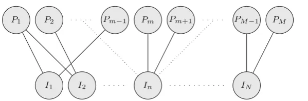
We consider a population ofNindividualsI1, . . . ,INwho can move between and potentially
interact on a number of Mdistinct places P1, . . . ,PM. The scenario can be illustrated as
bipartite graphs as in Fig.1where a link connects an individual In and a placePm if and
only if the place Pm can be visited by individual In [6]. A collection of all places Pm
that can be visited by an individual In will be called theterritoryof In and denoted by Pn = {m;Incan go toPm}. LetIm denote the set of individuals that can go to placePm,
i.e.Im = {n;Incan go toPm}, which we shall call the (potential)visitorsto Pm. If every
individual can go everywhere, we will call the populationunstructured.
The individuals play the game as follows. Each individualIn chooses a place Pm in its
I1 I2 In IN
P1 P2 Pm−1 Pm Pm+1 PM−1 PM
Fig. 1 General situation represented as a bipartite graph. A link connects an individualInand a placePmif
and only if the placePmcan be visited by individualIn
Pm, it receives a rewardRm(km)(sometimes later denoted just byRm) that, for the purpose
of this paper, depends solely on the place,Pm, and the (total) number of individuals,km,
occupying the place. Specifically, the reward does not depend on which individuals share the place and how the other individuals are distributed on the other places; we shall call this the
local aggregationassumption.
Unpacking this assumption, we are assuming the following. Places can be different of differing quality and of differing accessibility to individuals. Individuals, however, can differ only in the fact that different individuals can (potentially) access different places. This means that once on a particular place, which individuals are there does not affect the payoffs, except through the size of the group. Individuals are only concerned about their immediate payoff, i.e. about what is happening at their current place (and not about what is/or is not happening at other places).
The strategic element of the game involves the movement of the different individuals; each can employ different moving strategies and their aim is to maximize their payoff.
2.2 Game Theoretical Definitions
In the setting of the Territorial Movement Game, we will use the following definitions which are just the appropriate modification of the usual game theoretical notions (see for an example [7]).
An individualpure strategyis the choice of a particular place in a territory.
Given the territorial restrictions, different individuals may have different sets of available strategies to employ.
Theoccupancy functionis a functionO: {1,2, . . . ,N} → {1,2, . . . ,M}wherePO(n)for
O(n)∈Pnis a place to which an individualInhas moved. For every such occupancy function,
we define itsdistribution functionas an orderedM-tuplekmmM=1withkm= |{n;O(n)=m}|
being the number of individuals at placePm.
We say that two occupancy functionsO1 andO2areone move apart (by an individual
In0) ifO1(n)=O2(n)for alln=n0whileO1(n0)=O2(n0), i.e. if the difference between the occupancies is exactly in one individual changing its position.
The occupancy functionOis termedstableif any individual would receive a lower payoff when it unilaterally changes its position (given the fixed positions of other individuals); i.e. if for everyn
RO(n)(kO(n)) >Rm(km+1), for allm ∈Pn\O(n). (1)
[image:4.439.76.376.50.149.2](i) if O,O∈O, then there is a sequenceO = O1,O2, . . . ,Ok = Oof elements inO
such that each pairOiandOi+1is one move apart.
(ii) for allO,O ∈ O that are one move apart by an individual In0, RO(n0)(kO(n0)) =
RO(n0)(kO(n0)),
(iii) for allO∈OandO∈/Othat are one move apart, there must be at least one individual
In0such thatOandOare one move apart byIn0andRO(n0)(kO(n0)) > RO(n0)(kO(n0)).
In general it does not make sense to talk about a stable distribution function, as opposed to a stable occupancy function. Two occupancy functions can have the same distribution function, but one may be stable and the other not, because the possible moves depend upon the sets of territories of the individuals at each of the places, which will be different for each occupancy function. The exception is for the well-mixed population, where the territory of each individual is the full set of places, and consequently if an occupancy function is stable, so is any other occupancy function with the same distribution. Thus for the well-mixed population we say that a distribution function isstableif any occupancy function with that distribution function (and hence all of them) is (are) stable.
Often when considering evolutionary game theory, we assume that we have so-called
generic games(see for example [3,7]). Essentially, assuming that payoffs are derived from the natural world with its underlying variation, we can treat each payoff as if it is the realisation of a random variable, and so we ignore special sets of parameters that would occur with probability 0. This is useful, as the most problematic mathematical cases often occur on such parameter sets. In particular, equalities of distinct payoffs can cause problems. Here we shall call a gamegenericif
Rm(km)=Rm(km), if and only ifkm=km andm=m (2)
i.e. if different patches yield different payoffs (irrespective of the group size) and the same patch yields different payoffs for different group sizes. In subsequent sections, we give results that hold for both generic and non-generic games where we can, but sometimes it has proved necessary to restrict ourselves to consideration of generic games only. We clearly indicate at the appropriate point whether generic games are assumed.
A stable occupancy function is always a stable set (of one element). If payoffs are constant and the population is unstructured, the set of all occupancies is a stable set. If the payoffs are generic, a stable set has only one element, and this element is a stable occupancy function.
In Sect.2.3, we shall see that there is always at least one stable occupancy function for our game, providing that the local aggregation assumption holds. This is not generally true if it does not hold, as we see in the following example.
Example 1 A stable occupancy function may not exist without the local aggregation assump-tion. Consider two individuals, a predator and its prey, both of whom can go to one of two available places. The first individual, the predator, wants to be with the prey, but the prey wants to avoid the predator. The predator receives payoff 1 (0) if it is (not) at the same place as the prey, the prey receives 0 (1) if it is (not) at the same place as the predator. Note that the payoffs depend on who else is on the place, not only on the number of occupants. Clearly, no pair of pure strategies form a stable occupancy function.
2.3 Existence of a Stable set for the Territorial Movement Game
Here we show that there is always at least one stable set for the Territorial Movement Game. We will consider two Markov processes on the set of all occupancy functions. For thestrong
kmmM=1) to an occupancyO(with a distribution functionkmmM=1) to be allowable if they are one move apart byn0and the individual In0 would improve its payoff. Thus, there is a
potential transition if and only if there arem1,m2∈ {1, . . . ,M}such that (i) Im1∩Im2= ∅, i.e. there is an individual that could go to bothPm1andPm2,
(ii) km1 =km1−1, i.e. the individual is (potentially) leavingPm1,
(iii) km2 =km2+1, i.e. the individual is (potentially) coming toPm2,
(iv) Rm1(km1) < Rm2(km2), i.e. the payoff the individual gets atPm2is higher than the one
it got atPm1and
(v) km=kmfor allm=m1,m2, i.e. nobody else has changed their position.
Note that for the strong process, there cannot be transition from the stateOtoOand from
OtoOfor any pair of states. Furthermore in the generic case, there is no potential transition under the strong process if and only ifOis stable.
For theweakMarkov process, we will consider a transition to be allowable if the conditions (i)–(v) are satisfied, but the inequality in (iv) is not strict. Note that in either process we do not specify the probability of a transition occurring, except that any allowable transition has probability greater than zero.
We shall show the existence of a stable set in two stages.
(a) Let us first defineAsto be the set of all absorbing states of the strong Markov process. We claim thatAs= ∅.
Suppose thatAs = ∅. Then we could easily find a cycle
O1,O2,O3, . . . ,OT = O1 such that transitions can occur fromOi toOi+1 in the strong Markov process. This yields the existence of the sequencesm1,tTt=−11andm2,t+1Tt=−11such that
Rm1,t(km1,t,t) <Rm2,t+1(km2,t+1,t+1) (3)
corresponding to the fact that at timet there werekm1,t,tindividuals in place Pm1,t and one
of them was able to improve its position by moving to place Pm2,t+1. For every transition
at stept, we will have one inequality (3). Let us now look at the sequencekm,ttT=1for a specificm. The sequence is generally constant with occasional jumps by±1. Any time an individual leaves a place Pm, we havekm,t > km,t+1 = km,t −1, and the term Rm(km,t)
appears on the left-hand side of an inequality (3). Similarly, any time an individual moved to placePm,km,t <km,t+1=km,t+1, the termRm(km,t+1)appears on the right-hand side of an inequality (3). Since the sequencekm,tTt=1begins and ends atkm,1, the term Rm(km,t)
has to appear on the left-hand side of (3) as many times as on the right-hand side of (3). So adding those inequalities together (for allt) yields a contradiction.
So, we have shown that there is at least one occupancyO ∈As. IfO,O ∈As are one move apart by an individualIn0, there is no transition fromO to O or from O toO in
the strong Markov process and thus condition (ii) for a stable set is satisfied for all pairs of elements inAs. Consequently, whenO,O∈As, there is a transition (both ways) under the weak Markov process betweenOandO.
(b) Now, letBw ⊂ As be the set of occupancies that cannot, after any finite number of transitions in the weak Markov process, reach the setAcs, the complement ofAs. As above, there must be an occupancy functionO ∈Bw; otherwise, we would again get a cycle (and although we could now potentially have equalities in (3), we would have at least one strict inequality).
SinceBw ⊂As,Bwsatisfies condition (ii) for a stable set. Now assume that it does not satisfy condition (iii), i.e. that there isO∈BwandO∈/Bw, i.e.OandOare one move by
fromOtoOin a weak Markov process, and thus, there is a sequence of transitions fromO
throughOto an element ofAc
s, a contradiction with the fact thatO∈Bw.
A maximal “connected” component ofBw(i.e. the set of occupancies which one can get from any element ofBwby a sequence of changes) is then a stable set.
Remark 1 Here we illustrated with an example the concept of the setsAs andBwfrom the proof above. Consider 80 individuals with unrestricted movements that can go to two patches with payoffsR1(80) = R2(80)=1 andR1(k)= R2(79−k) =0 for 0 ≤k ≤79. Then
As corresponds to the set of all states but79,1or1,79andBwconsists of80,0and
0,80.
Whilst the above results hold for generic and non-generic games, the results from here until the end of Sect.2.3apply to generic games only.
Remark 2 For the generic territorial movement game, consider the algorithm “start with any occupancy function, and make transitions as in the strong Markov process until no further moves can be made”. As previously noted, for the generic case this yields a stable occupancy function. However, there may be of the order of MN occupancy functions and thus the
algorithm can take a long time to finish. We note that whichOis chosen next will in general depend upon the transition probabilities of the strong Markov process, which would need to be specified.
Unfortunately, it is not the case that the maximum improvement decreases every step and it cannot thus be used as an indicator of the fact that the process is already converging to the stable state. For example, consider a population of two individuals. IndividualI1, currently atP1can go toP1andP2, individualI2, currently atP2can go toP2andP3. Let the payoffs beR1(1)=0.5,R2(1)=1,R2(2)=0.51,R3(1)=0.99. The only improvement that can be made is that individual I1 moves from place P1 to place P2, increasing its payoff by 0.01. That move, however, sharply decreases the payoff of individualI2fromR2(1)=1 to
R2(2)=0.51. The next move would be by individualI2fromP2toP3, increasing its payoff by 0.48 toR3(1)=0.99.
Remark 3 An alternative way to show the existence of a stable occupancy function in the special case of the predator dilution game is shown in Sect.4.3.
We have shown here that there is at least one stable occupancy function, but in general there may be many, as we see in the following example.
Example 2 Consider a game where individuals prefer to be in groups of even numbers, and the payoff to an individual is 1 (0) if it is (not) in a group of even-numbered size. Let there be 2nindividuals andmplaces such that all individuals can go to all places. The number of distributions of individuals over the places is2nm+−m1−1(see [7] Exercise 9.1). The number of stable distributions can be obtained by sending individuals to places in pairs, yieldingn+mm−−11 stable states. Ifnm, then the number of distributions is roughly(2n)m−1/((m−1)!)and the number of stable distributions is(n)m−1/((m−1)!)so the proportion of stable distributions is 21−m.
3 A Habitat Selection Game
3.1 Game Setting
ConsiderMplacesP1,P2, . . . ,PMandNindividualsI1, . . . ,IN. If there arekmindividuals
at placePm, the payoff to each of these individuals will be
Rm(km)=Bm− fm(km) (4)
whereBm >0 is the basic suitability of placePmand fm is a nonnegative, increasing and
continuous function, with fm(0)=0. This corresponds to selecting a habitat to forage on,
and as the number of individuals on a given patch increases, the actual yield of the patch decreases. However, the yield does not depend on the particular occupants of the patch. In the unstructured population case where every individual can go everywhere, the game has been described for example in Cressman et al. [10], see also Kˇrivan et al. [23].
3.2 A Unique Distribution in an Unstructured Population
The following reasoning, up until the end of Sect.3, applies to both generic and non-generic games; note, however, that as shown in Remark 4 below, we do not necessarily have unique-ness in non-generic cases. A known solution to this game for effectively infinite populations is the so-called ideal free distribution [14] (ideal = rational individuals, free = no cost or restric-tion on movement). Typically, condirestric-tional on being at a particular place, the individuals want to be with as few other individuals as possible.
(a) Firstly, we show how to find a solution to the habitat selection game in finite unstruc-tured population. Rather than assuming that individuals all make their choice at the same time, let the individuals choose sequentially. The first individual will choose a placePm1that
yields the highest payoff; i.e.
Rm1(1)≥ max m=m1
{Rm(1)}. (5)
Clearly, individualI1cannot do any better; and if no other individual arrives, we have the stable occupancy function if there is a strict inequality in (5), i.e. a unique place with best reward. If there arek places which satisfy (5), then there will be a stable set includingk
distinct occupancy functions. In this case, assuming thatN ≥k, the firstkindividuals must choose thek solutions to (5), since after each choice, the value of the chosen place will decrease, and no longer yield the highest payoff to subsequent individuals. Now, assume that individualsI1,I2, . . . ,Ii made their choices in a sequence, so that there arekmindividuals
at placePmand that no individual could do better by unilaterally moving to a different place.
The individualIi+1will pickPmi+1such that
Rmi+1(kmi+1+1)≥ max m=mi+1
{Rm(km+1)}. (6)
Clearly, in addition to individualIi+1being unable to increase its reward, none of the other individualsIj forj <i+1 can increase their reward by unilaterally moving to a different
place either. Indeed, ifIi+1went to the same place asIj, thenIjmust be at the best possible
position it could now be (otherwise,Ii+1would have chosen a different one). Also, ifIj is
I1 I2 I3
P1 P2 P3 P4
1st 2nd 3rd
I1 I2 I3
P1 P2 P3 P4
3rd 2nd 1st
I1 I2 I3
P1 P2 P3 P4
1st 3rd 2nd
(c) (b)
(a)
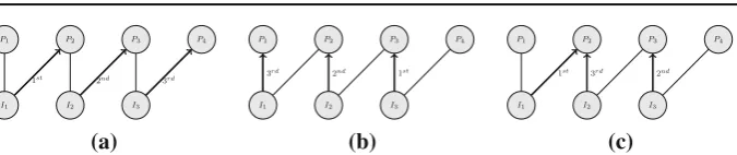
Fig. 2 Method showing the existence for the habitat selection game in an unstructured population cannot
be adopted for structured populations. In all instances, we assume that the payoffs are such thatR2(1) >
R3(1) >R4(1)> R1(1) > R2(2) >R3(2).aandbshow different stable occupancy functions for different orders at which individuals choose their places.cShows that there is an order under which no stable occupancy is reached (one can still follow the procedures from Sect.2.3to reach a stable occupancy function in several steps)
at other places have not changed). In this way, we can continue to place the individuals until all have made a choice.
(b) Now we show that while there will usually be many stable occupancy functions (depending on the sequence in which the individuals will make their choice), in unstruc-tured populations and generic games, these will all yield the same distributionkmMm=1.
To see the last statement, assume to the contrary that two stable occupancy functionsO
andOyield different distributionsk = kmMm=1andk= kmmM=1. Becausek=kand
mkm=
mkm, there must bem1andm2such thatkm1 >km1andkm2 <k
m2. Since the
payoffsRm1andRm2are monotone, we have
Rm2(km2+1)≥Rm2(km2 ), (7)
Rm1(km1+1)≥Rm1(km1). (8)
SinceOandOare stable occupancy functions, we have
Rm1(km1) >Rm2(km2+1), (9)
Rm2(km2) >Rm1(km1 +1). (10)
Thus, by (7), (8), (9), and (10), we get Rm1(km1) > Rm1(km1)which is a contradiction.
Consequently, the stable occupancy functionsOandOmust yield the same distributionsk
andk.
Remark 4 In a non-generic game, different occupancies (even in the same stable set) may yield different distributions. For example, consider an unstructured population of three indi-viduals and two places withR1(1) > R1(2) > R1(3) = R2(1) > R2(2) > R2(3). Then occupancies yielding a distribution3,0and a distribution2,1are both in the same stable set.
Remark 5 It seems that the same method as presented above would work for the case where individuals could visit only some of the places; the only modification needed being to take the maximum in (5) and (6) only over the allowable places. This is not the case, however, as shown in Fig.2. Consequently, we have seen that even the well-understood habitat selection game can get more complex if we put restrictions on individual movements.
[image:9.439.54.392.44.115.2]4 A Predator Dilution Game
4.1 Game Setting
ConsiderMplacesP1,P2, . . . ,PMandNindividualsI1, . . . ,INeach of which can move to
some (but potentially not all) of the places where the payoffsRm(km)are increasing functions
ofkm. This corresponds to the following scenario. Each day each individual selects a place. At
some point during the day, a predator arrives in the general area, picks a place at random (i.e. with probability 1/M) and attempts to eat one individual that is on that place. Each individual at the chosen placePmis equally likely to be eaten, with probabilityλm/(1+λmkm), using
the Holling type II predation function Kˇrivan [18], whereλmcorresponds to the rate at which
the predator finds any given prey (assuming unit available searching time). If there is no individual present, the predator stays hungry. Note that we assume that, unlike in [24], there is no refuge, i.e.λm>0 for allm.
The individual payoff for staying at placePmis thus
Rm(km)=Bm−
1
M
λm
1+λmkm,
(11)
whereBmis a baseline payoff. Many other payoff functions are possible, as long asRmare
all increasing functions ofkm.
In contrast to the habitat selection game, the individuals are now better off if they aggregate (although this would not be the case for a Holling type III function, see for example Garay and Móri [16]). In particular, in the special case where all places are of identical quality and individuals can go to all places, there can beMstable occupancy functions (each with a unique distribution), corresponding to all individuals being at a single place (in contrast to the habitat selection game when different stable occupancy functions yield the same distribution). Note that if we assumed that the predator keeps searching until it finds an occupied patch, the payoff to an individual could depend on the positions of others and thus violate the local aggregation assumption. For example, consider the case with largeN andMwithN ≤M, and a focal individual being alone. The payoff to the focal individual would be different if the others are all together (it will be killed with probability 1/2) or if they are all alone (it would be killed with probability 1/N). For our game defined above, this probability is 1/M
irrespective of the distribution of the others (as long as they are at different places to the focal individual).
4.2 All Solutions to the Predator Dilution Game
Here we present a method of finding all possible stable occupancy functions of the predator dilution game. The methodology in this section applies to generic games only. The fundamen-tal feature of the payoffs is that they increase with group size. Consequently, the individuals will want to aggregate as much as possible. In other words, they will try to fill up an already occupied place to its maximal capacity.
(a) Let us pick a permutationπon indices 1,2, . . . ,Mand define the occupancy function
Oby filling the places to the maximum in the order prescribed by the permutation as follows. We partition{1,2, . . . ,N}into a disjoint union of{UmI;m=1, . . . ,M}where
UI
UI
m=Iπ(m)\ m−1
m=1
Iπ(m);1<m≤M. (13)
In the above,U1I corresponds to all individuals that can go toPπ(1)andUmI corresponds to
all individuals that can go toPπ(m)but not to anyPπ(m)form<m. Define
O(n)=π(m); whenevern∈UmI (14) This yields a distributionkπ(m) = |UmI|. To check for the stability of O, first note that an
individual inPπ(j)cannot physically move to Pπ(i)fori < j (since ifO(n)=π(j), then
n∈UIj and thusn∈/Iπ(i)). Consequently, an occupancyOwill be stable if and only if
Rπ(i)(kπ(i)) >Rπ(j)(kπ(j))wheneveri< jandIπ(i)∪Iπ(j)= ∅. (15) (b) We claim that by going through all the permutationsπ, identifying the partitions{UmI}, defining the occupancy functions by (14) and discarding any non-stable ones (those that do not satisfy (15)), we will get all the stable occupancy functions.
First, it is clear that any occupancy function we get by the above procedure is stable. Conversely, ifO is a stable occupancy function with the distributionkmmM=1, consider a permutationπso that the sequenceRπ(m)(kπ(m))mM=1is decreasing. The placePπ(1)must be fully occupied; otherwise, any individual inIπ(1)but not currently at Pπ(1) would do better by moving toPπ(1)since for allm
Rπ(1)(kπ(1)+1) >Rπ(1)(kπ(1))≥Rm(km). (16)
Consequently, all individuals withPπ(1)in their territory must go there. Similarly, the remain-ing individuals with Pπ(2)in their territory have to go to Pπ(2) and so on. So, the above procedure with the permutationπindeed recovers the stable occupancy functionD, and any stable distribution which satisfies (15) must have an occupancy function defined by (12) and (13).
4.3 Existence of Stable Occupancy Functions for the Predator Dilution Game
Following Sect.2, we know that there is at least one stable set (a stable state for the generic game) for the general territorial movement game, and so in particular for the predator dilution game. In Sect.4.2, we have seen a way of finding all solutions to the predator dilution game, but there may be few or many, and each case needs to be searched one by one. Here we show a method to efficiently find at least one solution to the predator dilution game (particularly useful for large populations/ structures).
The existence of stable occupancy functions for the Territorial Movement Game has been already shown in Sect.2.3. However, due to the monotonicity of rewards in the predator dilution game, we can provide an explicit recursive method to identify a stable occupancy function.
We will define a permutationπon{1, . . . ,M}as follows. At the beginning, consider that all individuals are unplaced and all places unoccupied, and so define the sets of unoccupied places and unplaced individuals at step 0 as
VI
0 = {1,2, . . . ,N}, (17)
VP
This means that onceVtI−1andVtP−1are defined, for somet≥1, we pickπ(t)∈VtP−1such that
Rπ(t)(|Iπ(t)∩VtI−1|)= max
m∈VP t−1
Rm(|Im∩VtI−1|). (19)
In principle, in (19) we may have to evaluateRm(0)for somemand for simplicity we define
it asRm(0)= −∞. Whenπ(t)is chosen, we define VI
t =VtI−1\Iπ(t)and (20)
VP
t =VtP−1\ {π(t)}, (21)
corresponding to the fact that now placePπ(t)is fully occupied and individuals that could go toPπ(t)are now placed.
We repeat the process untilVtI = ∅. Since we are filling the places to their maximum,
VP
t = ∅impliesVtI= ∅. Also, each step of the above procedure will make exactly one more
place occupied and we are also assigning at least one individual to such a place. Consequently, the procedure is well defined and will stop in no more than min{N,M}steps. If the above procedure has not definedπon the whole{1, . . . ,M}, we will just defineπto be the (unique) increasing numerical sequence on the remaining elements.
Once the permutationπis defined, we use it to construct the occupancy functionO as done earlier in Sect.4.2by (14) together with (12) and (13). The occupancy function Ois clearly stable. Indeed, the individuals that go toPπ(1)cannot do any better as this place is fully occupied and it is the place that yields a payoff higher than at any other fully (and thus also arbitrarily) occupied place. The individuals at placePπ(2)also cannot do any better, because they cannot move toPπ(1)but are at the place that is fully occupied and yields the highest reward of all other places occupied fully (and thus also arbitrarily) by those that cannot go toPπ(1); and so on.
5 Discussion
In this paper, we have considered the important problem of how groups of animals should allocate themselves between different habitats, introducing a method to model this using a finite population, where the movement of the individuals faces some restriction. We have considered the general case, showing that there is at least one stable population distribution, but there can be many. We have also considered a development of the classical ideal free distribution of optimal foraging to our structure and developed a model of predator dilu-tion; in each case, we have shown how to find the stable occupancy functions (and that the corresponding distribution is unique in the case of unrestricted movement for the generic case).
that it would be replicated from group to group within the overall population, and so some more complicated scenario with many possible structures might be needed.
This model reflects real cases where foraging is restricted. An example would be polli-nators (as the individuals) and plants (as the places), where each pollinator specialises in a subset of the available plants and some plants specialize for certain pollinators [20,44]. Here the “territories” of individuals are not physical areas in space, but their own set of host plants. It can also be used to model more general situations, which are not principally about foraging. A range of activities that apply to group-living animals can be regarded in this way, for example taking shelter, or migration (where a “place” would be a migration route) or alternatively mating, where the females may be considered as individuals and the males as “places”. Currently our model is very general, but it is flexible, and there is the potential to develop it to model more species-specific situations.
There are a number of ways that the modelling in this paper can be developed. One can relax the local aggregation assumption as done for example in Maciejewski and Puleo [29] where authors consider a structured population model where different individuals are best suited to different regions of their environment. Also, in this paper we have assumed strategies are pure, so that each individual chooses a place so that given the individuals choices the occupancy function is determined. An interesting question is, can there be mixed strategies, where individuals choose a place according to a probability distribution? We note that a population with only two individuals moving toMpatches is a form of bi-matrix game (with special payoffs). ESSs in such games are always pure, following the work of Selten [38]. When can this result be generalised to our multi-player case, meaning that no mixed strategy could be stable? It would also be of interest to consider general, and specific, models on structures of movement with special properties. Models in evolutionary graph theory have focused on such ideas to significant benefit, and there is potential in our model too.
Acknowledgments This work was supported by funding from the European Unions Horizon 2020 research and innovation programme under the Marie Skodowska-Curie Grant Agreement No 690817. The research was also supported by the Simons Foundation Grant 245400 to J. Rychtáˇr. The authors also would like to thank V. Kˇrivan for his comments and suggestions that helped to improve the quality of the paper.
Open Access This article is distributed under the terms of the Creative Commons Attribution 4.0
Interna-tional License (http://creativecommons.org/licenses/by/4.0/), which permits unrestricted use, distribution, and reproduction in any medium, provided you give appropriate credit to the original author(s) and the source, provide a link to the Creative Commons license, and indicate if changes were made.
References
1. Allen B, Nowak MA (2014) Games on graphs. EMS Surveys Math Sci 1(1):113–151
2. Antal T, Scheuring I (2006) Fixation of strategies for an evolutionary game in finite populations. Bull Math Biol 68(8):1923–1944
3. Binmore K, Samuelson L (2001) Can mixed strategies be stable in asymmetric games? J Theor Biol 210(1):1–14
4. Broom M, Lafaye C, Pattni K, Rychtáˇr J (2015) A study of the dynamics of multi-player games on small networks using territorial interactions. J Math Biol 71(6–7):1551–1574
5. Broom M, Rychtáˇr J (2008) An analysis of the fixation probability of a mutant on special classes of non-directed graphs. Proc R Soc A Math Phys Eng Sc 464(2098):2609–2627
6. Broom M, Rychtáˇr J (2012) A general framework for analysing multiplayer games in networks using territorial interactions as a case study. J Theor Biol 302:70–80
7. Broom M, Rychtáˇr J (2013) Game-theoretical models in biology. CRC Press, Boca Raton
8. Bruni M, Broom M, Rychtáˇr J (2013) Analysing territorial models on graphs. Involv J Math 7(2):129–149 9. Cantrell RS, Cosner C, Lou Y (2010) Evolution of dispersal and the ideal free distribution. Math Biosci
Eng MBE 7(1):17–36
10. Cressman R, Kˇrivan V, Garay J (2004) Ideal free distributions, evolutionary games, and population dynamics in multiple-species environments. Am Nat 164(4):473–489
11. Cressman R, Kˇrivan V (2010) The ideal free distribution as an evolutionarily stable state in density-dependent population games. Oikos 119(8):1231–1242
12. Cressman R, Tran T (2015) The ideal free distribution and evolutionary stability in habitat selection games with linear fitness and allee effect. Interdis Top Appl Math Springer Model Comput Sci, pp 457–463 13. Fretwell SD (1972) Populations in a seasonal environment, vol 5. Princeton University Press, Princeton 14. Fretwell S, Lucas H (1969) On territorial behavior and other factors influencing habitat distribution in
birds. Acta Biotheor 19(1):16–32
15. Garay J, Cressman R, Xu F, Varga Z, Cabello T (2015) Optimal forager against ideal free distributed prey. Am Nat 186(1):111–122
16. Garay J, Móri T (2010) When is predator’s opportunism remunerative? Commun Ecol 11(2):160–170 17. Hadjichrysanthou C, Broom M, Rychtáˇr J (2011) Evolutionary games on star graphs under various
updating rules. Dyn Games Appl 1(3):386–407
18. Holling C (1959) The components of predation as revealed by a study of small-mammal predation of the European pine sawfly. Can Entomol 91(05):293–320
19. Houston A, McNamara J (1988) The ideal free distribution when competitive abilities differ: an approach based on statistical mechanics. Anim Behav 36(1):166–174
20. Johnson SD, Steiner KE (2000) Generalization versus specialization in plant pollination systems. Trends Ecol Evol 15(4):140–143
21. Krause J, Ruxton GD (2002) Living in groups. Oxford University Press, Oxford
22. Krijger C, Sevenster J (2001) Higher species diversity explained by stronger spatial aggregation across six neotropical drosophila communities. Ecol Lett 4(2):106–115
23. Kˇrivan V, Cressman R, Schneider C (2008) The ideal free distribution: a review and synthesis of the game-theoretic perspective. Theor Popul Biol 73(3):403–425
24. Kˇrivan V (2013) Behavioral refuges and predator-prey coexistence. J Theor Biol 339:112–121 25. Kˇrivan V (2014) The allee-type ideal free distribution. J Math Biol 69(6–7):1497–1513
26. Lieberman E, Hauert C, Nowak M (2005) Evolutionary dynamics on graphs. Nature 433(7023):312–316 27. Maciejewski W (2014) Reproductive value in graph-structured populations. J Theor Biol 340:285–293 28. Maciejewski W, Fu F, Hauert C (2014) Evolutionary game dynamics in populations with heterogenous
29. Maciejewski W, Puleo GJ (2014) Environmental evolutionary graph theory. J Theor Biol 360:117–128 30. Maynard Smith J (1982) Evolution and the theory of games. Cambridge University Press, Cambridge 31. Morris DW (1988) Habitat-dependent population regulation and community structure. Evol Ecol
2(3):253–269
32. Morris DW (2002) Measuring the Allee effect: positive density dependence in small mammals. Ecology 83(1):14–20
33. Nowak M (2006) Evolutionary dynamics: exploring the equations of life. Belknap Press, Harvard 34. Ohtsuki H, Hauert C, Lieberman E, Nowak M (2006) A simple rule for the evolution of cooperation on
graphs. Nature 441(7092):502
35. Parker G (1978) Searching for mate. In: Sibly RM, S R (eds) Behavioural ecology: ecological conse-quences of adaptive behaviour. Blackwells, Oxford, pp 214–244
36. Prokopy RJ, Roitberg BD (2001) Joining and avoidance behavior in nonsocial insects. Annu Rev Entomol 46(1):631–665
37. Santos F, Pacheco J (2006) A new route to the evolution of cooperation. J Evol Biol 19(3):726–733 38. Selten R (1980) A note on evolutionarily stable strategies in asymmetric animal conflicts. J Theor Biol
84:93–101
39. Steele WK, Hockey PA (1995) Factors influencing rate and success of intraspecific kleptoparasitism among kelp gulls (larus dominicanus). Auk 112(4):847–859
40. Sutherland W, Parker G (1985) Distribution of unequal competitors. In: Sibly RM, S R (eds) Behavioural ecology: ecological consequences of adaptive behaviour. Blackwells, Oxford, pp 255–274
41. Voelkl B (2010) The “Hawk-Dove” game and the speed of the evolutionary process in small heterogeneous populations. Games 1(2):103–116
42. Voorhees B (2013) Birth–death fixation probabilities for structured populations. Proc R Soc Lond A Math Phys Eng Sci R Soc 469:20120248
43. Voorhees B, Murray A (2013) Fixation probabilities for simple digraphs. Proc R Soc A Math Phys Eng Sci 469(2154):20120,676
44. Waser NM, Ollerton J (2006) Plant-pollinator interactions: from specialization to generalization. Univer-sity of Chicago Press, Chicago
45. Woodroffe R, Ginsberg J, Macdonald D (1997) The African wild dog: status survey and conservation action plan. World Conservation Union, Gland