Three-fund Constant Proportion Portfolio Insurance Strategy
Ze Chena, Bingzheng Chena, Yi Hub and Hai Zhangc1
a School of Economics and Management, Tsinghua University,Beijing, China;b Hanqing Advanced
Institute of Economics and Finance, Renmin University, Beijing, China;c Department of Accounting &
Finance, Strathclyde Business School, UK
Abstract
Specific purpose guarantee funds (SPGFs) such as pension guarantee funds are becoming much popular among loss averse investors with common peculiar investment purpose, but receive few academic attention regarding to its investment strategy, hedging technique and performance. In this paper we propose a more practical constant proportion port-folio insurance (CPPI) strategy, three-fund CPPI (hereafter 3F-CPPI) strategy, which optimally allocates its assets in three funds: a risk-free fund, a stock-index fund and a purpose-related stock fund, to maximize the loss averse investor’s utility and to control the downside risk as well. Closed-form solutions of the optimal allocations of 3F-CPPI and its outcome distribution have been derived first under the continuous time case, fol-lowed by an extensive Monte Carlo simulation under the discrete time case to compare 3F-CPPI with other benchmark strategies such as CPPI. Our simulation results show that the proposed 3F-CPPI dominates other benchmark strategies in almost all the aspects such as the mean return, downside risk control and loss averse utility.
Keywords: Portfolio insurance strategies; Specific purpose guarantee funds; CPPI; 3F-CPPI.
1. Introduction
There is an increasing number of funds whose investors anticipate a minimum guar-anteed return and plan a specific intended use of the investment, which is called special purpose guarantee funds (SPGFs henceforth). Take the retirement purpose as an in-stance, one typical SPGFs is the guaranteed minimum income benefit (GMIB) annuity fund, which provides life-long pension payments to investors after retirement and guar-antees a certain one-off payment in the case of early death. Another SPGFs example is children future education expense fund, such as F&C’s Children’s Investment Plan, which enables parents to contribute a monthly or lump sum investment today to cover children’s education-related expenses in years, like the college education costs. The price inflation with respect to the specific purpose of the investment outcome makes the SPGFs different
Table 1: The difference between CPPI and 3F-CPPI
Composition Objective Allocation Strategy
CPPI 3F-CPPI Floor (risk-free) guaranteed return a risk-free fund X X
Cushion (risky) excess return a market index fund X X
a special sector index fund X
from an ordinary guarantee fund. The SPGFs investors are expecting a minimum guar-anteed return and achieve a high purchase power of the investment outcome at maturity as well.
Although there are many types of SPGFs promising a minimum guaranteed return participated by investors with a specific use of the investment, few academic attention is paid to SPGFs’ investment strategy, hedging techniques and its performance. For instance, GMIB annuity fund adopts only the CPPI strategy under the regulation of Insurance Regulation Commission (CIRC) providing life-long pension to its investors. CPPI dynamically allocates the funds on two funds, a risk-free fund and a risky one such as stock index fund, to achieve a guaranteed return during the investment period. However, CPPI strategy does not consider any purpose related risks, an essential factor affecting the valuation of SPGFs for loss averse investors. Thus it is inappropriate and impractical for SPGFs loss averse investors to adopt only the standard CPPI strategy. Therefore, we firstly propose an adjusted CPPI strategy, 3F-CPPI, which allocates its fund into not only a risk free asset and a risky portfolio but an extra purpose-related asset with the aim of hedging against specific risks such as purpose-related inflation.
Investing in a third fund within an adjusted CPPI strategy has also been justified by the high correlation between the purpose related inflation risk and the performance of specific industry stocks. A bunch of empirical studies examine the relationship between price inflation and stock return, which further justifies the feasibility of hedging inflation risk by investing in highly correlated stocks. For example, a robust relationship has been found between the inflation and certain industry sector stocks including the financial sector stocks (Boyd et al., 2001), oil and gas industry sector stocks (Sadorsky, 2001;
Apergis and Miller, 2009; Kang et al., 2015) and real estate and real estate investment trusts (REIT) (Rubens et al., 1989; Hoesli and Oikarinen, 2012; Bahram et al., 2004). Thus, a natural way to hedge the inflation risk and maintain a relative stable purchase power for SPGF investors is to allocate some assets into purpose-related stocks. As indicated in Table 1, the main difference between CPPI and 3F-CPPI is that 3F-CPPI invests in three funds: a risk-free fund, a second risky fund (e.g. market index fund) and a third fund for hedging specific risks (e.g. industry stock fund). Intuitively, the proposed 3F-CPPI strategy ensures a guaranteed performance while the funds allocated on the third asset hedges the specific risk for the loss averse investors.
variable proportion portfolio insurance (VPPI) outperform the standard CPPI.Chen et al.
(2008) propose a dynamic proportion portfolio insurance (DPPI) strategy by identifying risk variables that are related to market conditions and used to build the equation tree for the risk multiplier by genetic programming.
Also as SPGFs investors tend to be loss averse, a feature which is quite different from the classical variance framework, thus mutual fund separation derived from mean-variance framework might be inappropriate for SPGFs. Dichtl and Drobetz (2011) find that the investors who prefer guarantee funds are proven to be loss averse and the popu-larity of PI strategies can only be explained in a behavioural finance context. The most popular CPPI strategy firstly proposed by Black and Jones(1987) and Black and Perold
(1992) is a two-fund investment strategy by investing assets into a risk-free fund and a diversified asset. The CPPI strategy seems to follow the logic or principle of the famous two-fund separation, however, they are not belong to the same investment categories. The two-fund separation is firstly developed by Tobin (1958) and Markowitz (1959) un-der a mean-variance framework, and further proved by Merton(1973) in continuous-time capital asset pricing model independent of preferences, wealth distribution, and time hori-zon. Nevertheless, there has been plenty much discussion questioning the hold of mutual fund separation: for instance, some literatures believe that when agents do not have mean-variance preferences or the investment opportunities are not constant, alternative assumptions are needed in support of mutual fund separation.2
Further, three-fund or even K-fund separation theorem has been developed as the invalidity of mutual fund separation.(Merton, 1973; Cairns et al., 2006; Dahlquist et al.,
2016; Dybvig and Liu, 2018). Our innovative solution for SPGFs by investing in an ex-tra fund is inspired by the loss aversion feature of SPGFs investors, a utility framework which is quite different from the classical mean-variance one. However, we do not claim 3F-CPPI is a direct application of three-fund separation theorem, neither do we state the optimal allocation strategy for SPGFs investors be necessarily 3F-CPPI. Most impor-tantly, proposing an innovative 3F-CPPI for loss averse SPGFs investors and testing its superiority over benchmark PI strategies are the main contributions of this paper.
Within the general portfolio insurance setting featuring loss averse utility, we have derived the explicit optimal allocation rule for the 3F-CPPI strategy and its final payoff distribution as well. Further extensive Monte Carlo simulations have been conducted to give further intuitive insights of 3F-CPPI’s superiority over other benchmark strategies. More specifically, the proposed 3F-CPPI strategy outperforms the standard CPPI and other strategies in various aspects such as mean return, expected fall and protection ratio etc. Despite both 3F-CPPI and CPPI are well able to hedge against the downside risk, 3F-CPPI proves to be superior to the CPPI strategy with regards to reshaping return distribution and investor’s utility. We prove further that the 3F-CPPI are most favoured by loss averse investors compared with other strategies.
The rest of the paper is structured as follows. Section 2 briefly introduces the financial market. An innovative 3F-CPPI strategy with closed-form solutions for its optimal
tion rules and leverage has been constructed in Section 3, followed by an extensive Monte Carlo simulations comparing the 3F-CPPI strategy among several contrastive strategies in Section 4. Finally, Section 5 concludes and the proof techniques can be found in the Appendix.
2. Financial market and loss averse utility
2.1. Financial market
First, a stock market index, denoted by StI, has been established using all n stocks in the financial market. Further, we assume the dynamic process of the stock index SI
t and
risk free asset Stf are captured by geometric Brownian motions as follows
dSI
t
SI
t
=µidt+σsidZs, (1)
dSf =rSfdt, (2)
where µi is the expected growth rate, σi is the volatility of the stock market, r is the
risk-free interest rate and Zs is the Brownian motion which drives the stock market.
We further assume there exists a market sector consisting of m (m < n) stocks and it is closely related to the special purpose of a given SPGFs. As in the example of pension funds, the sector that consists medicine and health-related industry stocks is defined as the purpose-related market sector. Similar to the stock market index, the dynamic process of the purpose-related market sector index, denoted by SP
t , is given by
dStP
SP
t
=µpdt+σspdZs+σppdZp
=µpdt+σPdZP, (3)
where Zs and Zp are two orthogonal Brownian motions, and σPdZP = σspdZs +σppdZp.
Thus, Brownian motion ZP is correlated withZs :
dZPdZs=
σs
p
q
(σs
p)2 + (σ p p)2
dt. (4)
TheSI
t fund andStP fund are driven by two different but correlated Brownian motions.
For simplicity, we hereafter refer the market index fundStIand the specific purpose related index SP
t toI-fund and P-fund respectively.
As the SPGFs’ payoff is to be used for a specific purpose such like hedging medical costs for pension funds, the inflation of purposed-related expense shall definitely reduce investors’ utility from the investment. More specifically, we denote the given SPGFs’ purpose related expense inflation index as Yt, and refer it to the purpose-related expense
We assume further Yt is jointly driven by stock market risk and other risk (e.g.
id-iosyncratic risk) that has not been traded in the stock market. The process of Yt is given
by:
dYt
Yt
=µydt+σysdZs+σypdZp+σeydZe, (5)
where Zi, Zp, Ze are orthogonal Brownian motions. It is noteworthy that Yt can not be
perfectly hedged by neither the I-fund nor the purpose-related P-fund.
By SDE process (5), one can write stochastic integration:
Yt=Y0exp{(µy −
1 2(σ
s y)
2− 1 2(σ
p y)
2− 1 2(σ
e y)
2)t+σs
yWst+σypWpt+σeyWet}
=Y0exp{µYt+σYWY t}, (6)
whereY0 = 1, andµY =µy−12(σyi)2−
1 2(σ
p y)2−
1 2(σ
e
y)2, σYWY t =σysWst+σypWpt+σyeWet.
So far, we have introduced SDE process of Yt, Zi and Zp, which are jointly driven by
three orthogonal BMs Zi, Zp and Ze. To write down as a unified form, we define:
dNt =µNdt+σnsdZs+σpndZp +σnedZe, (7)
whereNt=StI, StP, Yt, andn=i, p, ycorrespondingly. −→σn = (σns, σnp, σen) is the volatility
vector of process of Nt, thus, −→σi = (σis, 0,0),
− →σ
p = (σps, σpp, 0) and
− →σ
y = (σys, σyp, σey).
2.2. Loss averse utility
Generally, investors of guaranteed funds tend to be loss averse, which explains the popularity of guaranteed funds and portfolio insurances (Dichtl and Drobetz, 2011). In contrast to the expected utility theory, the guaranteed fund investors are proven to be loss averse with the following behavioural characteristics: 1. evaluate investment outcome by its deviation from some specific reference point; 2. value potential gains and losses asymmetrically, i.e. the marginal utility of the potential is higher than that of the gains. Therefore, we adopt the loss averse utility defined as follows in our framework.
More specifically, loss averse investors have an S-shaped utility function being concave for gains and convex for losses. Investment outcome has been considered as either positive or negative deviations from a reference point. Following Dichtl and Drobetz (2011) and
Tversky and Kahneman (1992), the loss averse utility function is defined as follows:
ν(∆V) =
(∆V)γ
−λ(−∆V)γ
for ∆V >0
for ∆V <0 , (8)
where ∆V is the deviation from reference point, 1 > γ > 0 and λ > 1. It’s noteworthy that the concave part of utility (8) is equivalent to the form of Constant Relative Risk Aversion (CRRA) utility 3 given by
uCRRA(∆V) = 1
γ(∆V)
γ, where 0 < γ <1. (9)
Due to the specific investment purpose, the investors’ utility is not only determined by the investment outcome, but also by the inflation of purpose-related expense, YT. As the
price index YT at maturity dramatically affects the real wealth level of the investment.
Similar to the concept of real income, the SPGFs investors’ utility or subject value of SPGFs should be deflated by the price inflation index as well.
After considering the purpose-related inflation risk, at time t, the SPGFs investor’s loss averse utility is defined as follows
U(VT, YT) =
(
(VT−PT
YT )
γ
−λ·(−VT−PT
YT )
γ
for VT >PT
for VT < PT
, (10)
where γ is the risk averse parameter of the SPGFs investors. The relative risk aversion
(RRA) coefficient of utility U(∆V) is R=−xU
00 2
U20 = 1−γ.
We add the reference point and the purpose-related inflation risk in our utility func-tion (10) for the following two reasons4. First, Dichtl and Drobetz (2011) demonstrates that the investors of guarantee funds are loss averse and the reference point is based on the principal investment which is related to the absolute return of the guarantee funds. Second, the impact of inflation on consumption or utility has been commonly captured as the denominator in most economic literature.
3. Three-fund CPPI strategy
In this section, we briefly review the standard CPPI strategy in 3.1, followed by a detailed construction of the innovative 3F-CPPI strategy in3.2. Further3.3 proposes the loss averse investors’ utility maximisation problem and presents explicitly results as well.
3.1. Standard CPPI strategy
Constant proportion portfolio insurance (CPPI) is a trading strategy that allows a portfolio to maintain an exposure to the upside potential of a risky asset while providing a capital guarantee against downside risk. The outcome of the CPPI strategy is somewhat similar to a call option. Since CPPI is firstly proposed by Black and Jones (1987), it is widely used in many guaranteed funds as it maintains the portfolio value above a certain predetermined level (floor) and allows upside potential as well.
CPPI, a self-financing strategy, not only guarantees a fixed payoff PT at maturity but
chases the upside potentials via dynamic trading using leverage as well. According to the CPPI strategy, the fund value Vt is invested on the risk free fund (often referred as
“floor”) and the mutual fund (the “cushion”). Denote Pt and Ct as the floor and cushion
invested at time t respectively, then, they satisfies
Ct=Vt−Pt, t∈[0, T]. (11)
We assume the capital amount to be guaranteed at maturity isPT, then a typical floor
strategy at timet is a fixed-rate floor, which is given by,
Pt =e−d(T−t)PT, t∈[0, T], (12)
whered is the required return by investors for risk free asset andd6r. Also dis referred as the fixed rate of floor strategy, and d < r reflects a conservative case which allocates more assets in the risk-free fund. The most common floor strategy is to allocate the minimum amount of assets into the risk-free fund, i.e. d = r, then the floor amount at time t is determined by
Pt=e−r(T−t)PT, t∈[0, T]. (13)
The cushion, the difference between portfolio value and floor, will be invested in the mutual fund i.e. I-fund. A CPPI portfolio usually leverages its cushion Ct to chase
higher return, and its leverage ratio m stays constant as “constant proportion”. Thus, the portfolio’s exposure in stock market Et is
Et=mCt=m(Vt−Pt), t∈[0, T], (14)
where m > 1. Constant proportion m is determined at the time 0 and stays constant during the investment horizon. The cushion value Ct fluctuates with the market, once it
approaches zero all the fund will be invested in the risk-free asset till the maturity.
Therefore, a standard CPPI strategy is, in fact, a two-fund separation investment. At any time t, we have:
• if Vt> Pt, the portfolio allocates amount Ptin the risk-free fund, and amountCt in
the I-fund with leverage m;
• if Vt 6Pt, the entire portfolio is invested in the risk-free fund.
If using time-continuous rebalancing, the CPPI fund value Vt never falls below the
guar-anteed floor.
3.2. Three-fund CPPI
The famous mutual fund theorem holds only for “normal” investors with mean-variance preference. Due to the invalidity of mutual fund separation in incomplete markets, we propose a 3F-CPPI strategy to hedge these risks in a general portfolio insurance setting as well.
denote Pt and Ct as the floor and the cushion respectively. Unlike CPPI, the cushion of
3F-CPPI fund is invested in two risky funds: theI-fund and the P-fund. Denote αas the proportion of cushion to be invested in I-fund, then the remaining 1−αpart is assigned toP-fund.
Define Vt as the SPGF value and its evolution is given by
dVt=Et[α
dSI
t
SI
t
+ (1−α)dS
P t
SP
t
] +Vt
dSf
Sf
−Etrdt, (15)
where Et =mCt is the exposure to the risky asset. Now we summarise our main results
in the following proposition:
Proposition 1. Under the continuous time setting, for t ∈ [0, T] a 3F-CPPI portfolio value at time t follows the distribution:
Vt =Pt+C0exp(Bt−
1
2At) + (r−d)
Z t
0
exp{Bt−Bξ−
1
2A(t−ξ)}Pξdξ, (16)
and the expected portfolio value of the 3F-CPPI portfolio at time t is
E(Vt) = Pt+C0eµBt+ (r−d)p0eµBt
1−e(d−µB)t
µB−d
, (17)
where A=m2α2σ2
i +m2(1−α)2σ2P + 2m2α(1−α)σpsσi and
Bt ={r+m[ασiθi+ (1−α)σPθP]}t+m[ασiWst+ (1−α)σPW pt];P0+C0 =V0.
Proof: The proof of proposition 1is in Appendix.
For simplicity and without loss of generalization, hereafter we consider only the most common floor strategy(d=r) for the proposed 3F-CPPI strategy. Then, based on Equa-tion (16), a 3F-CPPI portfolio value at time t follows the following distribution
Vt =Pt+C0exp{{r+m[ασiθi+ (1−α)σPθP]−
1
2A}t+mασiWst+ (1−α)σPWP t}. (18) In fact, the CPPI can be viewed as a special case of 3F-CPPI with α = 1 and the distribution of a CPPI portfolio value at time t is
Vt =Pt+C0exp(Bt−
1 2m
2σ2
it) + (r−d)
Z t
0
exp{Bt−Bξ−
1 2m
2σ2
i(t−ξ)}Pξdξ, (19)
where Bt={(r+mσiθi)t+mσiQWst}, t ∈[0, T].
3.3. Optimal 3F-CPPI allocation rules
Suppose a SPGFs manager aims to maximize the investor’s utility U(VT, YT) in (10)
by choosing leverage m and I-fund proportion α at the commence of the fund. The optimization problem is given by
M ax
m,α E[U(VT, YT)|F0] (20)
⇐⇒ M ax
m,α E[U(
VT −RT
YT
To determine the optimal allocation (α∗, m∗), we first introduce the purpose-related risk-aversion adjusted return (PRA return henceforth). The PRA return is a modified indicator which reflects the effect of risk aversion and purpose-related inflation risk on evaluating the I-fund andP-fund.
Definition 1. For the stock index I-fund and purpose-related market sector P-fund, the purpose-related risk-aversion adjusted return (PRA return) is:
µ(nγ) =µn−γ→−σn· −→σy, n=i, p. (22)
where −→σn = (σns, σpn, σne), −→σy = (σys, σpy, σye).
In the definition of risk-aversion adjusted return, −→σn· −→σy is always positive. The
possible range of γ for loss averse investors is 0 < γ 61, thus there always is µ(nγ) 6µn.
The “punishment” of I-fund or P-fund increases with investors’ risk aversion and the fund’s volatility’s vector correlation with inflation Yt. Thanks to the concept of PRA
return, we solve the global optimal allocation parameters m∗ and α∗ of the 3F-CPPI portfolio as follows:
Proposition 2. The optimal allocation parameters m∗ and α∗ of the 3F-CPPI portfolio satisfy
F(m∗) = 0, (23)
α∗ =α∗(m∗), (24)
where
F(m) =α∗(m)µi(γ)+ (1−α∗(m))µp(γ)−r+ (µ(iγ)−µp(γ))α∗(m) (25)
+ (γ−1){[(σ
s
p)2+ (σpp)2−σpsσsi
(σs
i −σps)2+ (σ p p)2
+ (σpp)2+ (σps)2]m−σiyσps−σypσpp}.
α∗(m) = (σ
s
p)2+ (σpp)2−σpsσis
(σs
i −σsp)2+ (σ p p)2
+ µ
(γ)
i −µ
(γ)
p
(σi−σsp)2+ (σ p p)2
1
(1−γ)m, (26)
Proof: The proof of proposition2 and expressions of optimal m∗ and α∗ are provided in Appendix.
Proposition 2 illustrates the optimal m∗ and α∗ without considering the limited pos-sible range of parameters in practise. However, in real-world scenarios, there is an upper bound of the leverage m because of the regulation and fund’s borrowing capability. Also the portfolio cannot be rebalanced continuously in practice due to the gap risk. Besides, the range ofαmay be limited to [0,1] because of the short-sale constraints. Therefore, we discuss further the optimal ratioα∗ for a given the leverage ratiomin the next subsection.
Now we look a special example of optimal 3F-CPPI allocation: the SPGFs participated by risk neutral investors case with γ = 1. We further assume the parameter ranges are:
According to the Proposition 2, the optimal 3F-CPPI in the risk-neutral case de-generates into the two-fund separation, the optimal allocation α∗ and m∗ are given as follows
α∗ =
1
α, α∈[0,1]
0
if µ(1)i −µ(1)p >0
if µ(1)i −µ(1)p = 0
if µ(1)i −µ(1)p <0
, (27)
and
m∗ =
M
m, m∈[1, M]
1
if α∗µ(iγ)+ (1−α∗)µ(pγ)−r >0
if α∗µ(iγ)+ (1−α∗)µ(pγ)−r= 0
if α∗µ(iγ)+ (1−α∗)µ(pγ)−r <0
, (28)
where the excess PRA return is αµ(1)i + (1−α)µ(1)p −r, and M is the maximum possible
value of m. Optimal allocation in (27) is intuitive in explaining the 3F-CPPI’s optimal allocation principle: the optimal proportionα∗depends on comparison of PRA returnµ(1)i
andµ(1)p to a great extent, and the optimal leveragem∗ is greatly influenced by portfolio’s
average excess PRA return, αµ(1)i + (1−α)µ(1)p −r.
3.3.1. Continuous time: optimal α∗ for given leverage m
Now we turn to determine the optimal proportion α∗ invested in I-fund for given leverage m. In practice, the leverage m is limited and even regulated because of gap risk. According to the findings from ?, Balder et al. (2009) and Dichtl and Drobetz
(2011) among others, the leverage has been found to have significant impact on the CPPI portfolio’s outcome and it is normally below 10. For example,Dichtl and Drobetz (2011) consider m 6 10 cases while? compares CPPI’s performances for m= 3, 4, 5 cases. For a given range of m (16m 610), we investigate the optimal proportion α∗.
Equation (26) shows the relation between optimal m∗ and α∗ without consideration of range, the following corollary reveals that the monotonicity of α∗(m) depends on the relativity of PRA return of I-fund and P-fund, µi(γ)−µ(pγ).
Corollary 1. Given a leverage m, the optimal ratio α∗(m) satisfies: (1) If µ(iγ)> µp(γ), then α∗(m) is a decreasing function of m;
(2) If µ(iγ)< µp(γ), then α∗(m) is an increasing function of m;
(3) If µ(iγ)=µp(γ), then α∗ is not correlated with m.
Proof: If µ(iγ) > µ(pγ), then α∗(m) is a function of m in form of m1 by (26), which is
decreasing function of m. The remaining proof is similar and trivial.
Corollary 1 shows a “diversification” effect of optimal allocations: α∗(m) gradually shifts to the fund with less PRA as the increase of leverage rationm. This is an interesting feature of optimal allocation, whose diversification offsets the risk caused by the high leverage.
are constraints on short-sale, then the parameters ranges are m ∈ [1, M] and α ∈ [0,1]. With consideration of the bounds, we have the following proposition 3, whose proof is trivial.
Proposition 3. For a regulated leverage m ∈[1, M], the optimal ratio α∗c(m)∈[0,1] is:
α∗c(m) =
1
α∗(m)
0
if α∗(m)>1 if α∗(m)∈[0,1]
if α∗(m)<0
. (29)
So far, we have only considered the optimal allocation in a continuous time case, under which the portfolio is continuously rebalanced. As the portfolio value never falls below the floor in the continuous time case, the investor’s loss averse feature does not play a role in optimal allocation.
3.3.2. Discrete time: optimal α∗ for given leverage m
Due to the constraints of the continuous time case, we here consider a more practical case, the discrete time case, under which the portfolio cannot be rebalanced continuously. In the discrete time case, there is a gap risk that the cushion value of 3F-CPPI fund might turn to a negative value between two rebalance time, which means the portfolio is failing to achieve the guaranteed return. Therefore, the investor’s loss aversion characteristic plays a vital role in determining the optimal allocation.
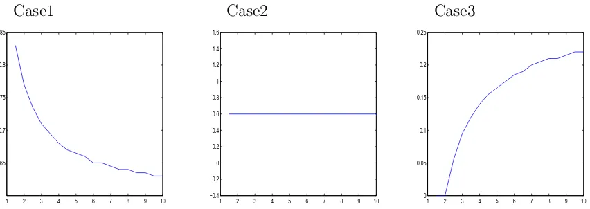
Monte Carlo simulation method is adopted to solve the optimal proportion α∗ for a given leveragem. Within the parameters ranges, for eachm, we run simulations through the range α ∈ [0,1] to search for the optimal α∗, the interval is 0.005. For each (m, α) pair, 100000 times simulations are run to calculate allocation outcome. In the simulation, we assign γ = 0.88, which is consistent with Tversky and Kahneman (1992) and Dichtl and Drobetz (2011). We consider the following three different scenarios of I-fund and
P-fund: 5
• Case 1: µ(iγ) > µ(pγ);
• Case 2: µ(iγ) =µ(pγ);
• Case 3: µ(iγ) < µ(pγ).
Figure 1 illustrates the relationship between optimal α∗ and leveragemfor these three cases, the interval of leveragemis [0,10]. The numerical results show the monotonic rela-tionship between optimalα∗ and leveragem in the discrete time case, which is consistent with the theoretical result. Having considering the gap risk in discrete time, the optimal allocation on I-fund and P-fund relies on the PRA return of the funds as well as the leverage m.
Case1
1 2 3 4 5 6 7 8 9 10 0.65
0.7 0.75 0.8 0.85
Case2
1 2 3 4 5 6 7 8 9 10 −0.4
−0.2 0 0.2 0.4 0.6 0.8 1 1.2 1.4 1.6
Case3
1 2 3 4 5 6 7 8 9 10 0
[image:12.612.86.512.63.214.2]0.05 0.1 0.15 0.2 0.25
Figure 1: The relationship between optimal allocationαand leveragemfor three different cases, i.e. Case 1 µ(iγ)> µp(γ), Case 2 µ(iγ)=µp(γ) and Case 3 µi(γ)< µ(pγ) .
3.4. An example: pension guarantee funds in China
Here we use an example of pension guarantee funds in China to show the advantage of the proposed 3F-CPPI strategy. The medical and health-related expense is one of the major parts of living cost for retirees in China, and its price inflation significantly affects the retiree’s utility of pension savings. Using historical data from Shanghai Stock Exchange, we simulate the performance for both the 3F-CPPI and CPPI strategy.
The IAMAC-SinoLife China Senior Living Cost Index (ISLCI) is a price index issued by Insurance Asset Management Association of China (IAMAC). It measures the living cost of retirees in mainland China. Figure 2 compares the ISLCI and CPI in the period from Jan 2001 to May 2017. As indicated in Figure 2, the annual increasing rate for ISLCI is 3.86% which is much higher than CPI with an annual increasing rate of 2.46%.
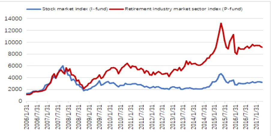
Meanwhile, within the period between January 2006 to May 2017, the performance of the stock market index (I-fund) and the retirement industry sector index (P-fund) in China have been illustrated in the Figure 3. Both the stock market index (I-fund) and the retirement industry sector index (P-fund) are calculated by daily traded stocks, issued by Shanghai Stock Exchange. Figure 3 shows the P-fund achieves a higher return than the I-fund during the time window selected.
Figure 2: Historical ISLCI and CPI in China from Jan 2001 to May 2017 (Source: Insur-ance Asset Management Association of China (IAMAC))
[image:13.612.74.527.406.633.2]Figure 4: Historical simulation: the performance of CPPI and 3F-CPPI portfolios
4. Simulation analysis
It is obvious that the 3F-CPPI dominates CPPI under the continuous time case as the latter can be viewed as a special case of 3F-CPPI. However, whether 3F-CPPI outperforms CPPI or other bench strategies under the discrete case with gap risk is not that obvious and needs further investigation.
In this section, we first start Monte Carlo simulation in Subsection4.1, followed by the detailed definitions of benchmark strategies and performance measures in Subsection4.2, the main results with regard to the performance of 3F-CPPI with other bench strategies such as CPPI are presented in Subsection 4.3.
4.1. Simulation Design
The Monte Carlo simulations are carried on a step-by-step basis as follows:
1. A wide range of the market possibilities with eight economic scenarios in total has been considered, including four different relativity of performance fromI-fund and
P-fund under two different inflation levels.
2. Then we run 100,000 simulation times for each scenario, the performance for 3F-CPPI and other benchmark strategies from Monte Carlo simulation has been re-ported.
According to the model in Section2, the stock market and the purpose-related inflation index follow multivariate correlated Brownian motion processes. Before running Monte Carlo simulation, some key parameters have to be assigned: the return and volatility of the I-fund : µi and −→σi; the return and volatility of theP-fund : µp, −→σp; and the growth
rate and volatility of the purpose-related expense risk: µy, −→σy.
We refer to the existing literature for assigning parameters value. Similar toArnott and Bernstein(2002), we first assume the risk free raterf is fixed at 4.5% within the investment
period. According to Dimson et al. (2008), the mean annual equity excess return for developed stock markets was approximately 7% between 1900 and 2005, resulting in an expected excess return around 4.5% per year. In our simulation, we then estimate that a high state of stock market excess return is 6.5%, and a low state is 4.5%. Last, Dimson et al. (2008) find the long-run stock return volatility was roughly 20% per year that has been used in simulation by other scholars likeBenninga(1990) andFiglewski et al.(1993). Therefore, we estimate the stock market volatility with a range from a high state of 30% to a low state of 20%.
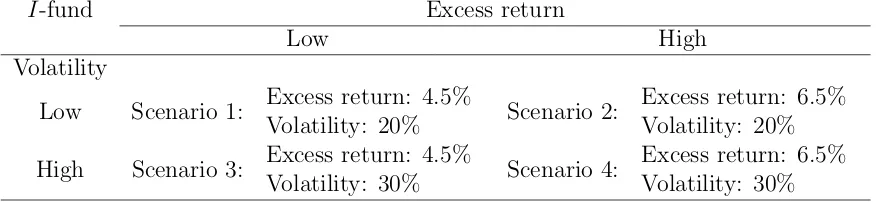
[image:15.612.79.519.427.528.2]As claimed in Section3, the 3F-CPPI optimal allocation depends mainly on the relativ-ity of I-fund and P-fund. To present a comprehensive analysis of 3F-CPPI performance, we consider four possible market scenarios with a fixed P-fund and four different I-fund market scenarios, the varied I-fund has either a higher (lower) return or a higher (lower) volatility than the given P-fund respectively. The four states of the stock market are summarized in Table 2.
Table 2: Four different market scenarios and a fixed performance ofP-fund with mean excess return and volatility of being 5.5% and 25% respectively
I-fund Excess return
Low High
Volatility
Low Scenario 1: Excess return: 4.5%
Volatility: 20% Scenario 2:
Excess return: 6.5% Volatility: 20%
High Scenario 3: Excess return: 4.5%
Volatility: 30% Scenario 4:
Excess return: 6.5% Volatility: 30%
Other than the stock market, the inflation index plays an important role in the eco-nomic scenarios. Unlike the highly volatile stock markets, the inflation is a more steady process. We distinguish it by low and high inflation states, which has been summarised as follows:
Low Inflation Trial: In four scenarios of the low inflation trial, we assume the mean growth rate and volatility of the inflation index Yt are 3% and 1% respectively.
High Inflation Trial: In four scenarios of the high inflation trial, we assume the mean growth rate and volatility of the inflation index Yt are 12% and 1% respectively.
We further assume the inflation index Yt has a different correlation with the I-fund
andP-fund in both trials: with the correlation betweenYtandI-fund return being 16.7%,
Similar to Benartzi and Thaler (1995) and Dichtl and Drobetz (2011), we consider a one-year investment horizon and simulate 250 daily observations for each scenario. The guarantee level of the SPGF is set to be 100% (full capital guarantee). We normalize the initial SPGFs value V0 as 100. We run 100,000 simulation times for each scenario to provide a stable and convincing test. T-test has been applied to compare performances among 3F-CPPI and other benchmark strategies. All portfolio insurance strategies in the simulation adopt a base case leverage of m = 5, which has been commonly used in practise (Herold et al., 2005).
4.2. Benchmark strategies and performance measures
4.2.1. Benchmark strategies
We select a variety of benchmark strategies, including CPPI, TIPP, stop-loss, buy-and-hold strategy and the risk-free investment, to test the superiority of the proposed 3F-CPPI.
CPPI strategies
CPPI strategy has been introduced in 3.1. The benchmark strategies consider two CPPI strategies with a difference in the risky fund: i.e. the risky asset of CPPI-I strategy is the
I-fund while that of the CPPI-P is the P-fund.
TIPP strategy
Time invariant portfolio protection (TIPP) strategy proposed by Estep and Kritzman
(1988), not only ensures a protection of the investor’s initial wealth but also any interim capital gains during the investment. Instead of having a fixed-rate floor like CPPI, TIPP’s floor is ratchet up with the value of the portfolio during the investment period. Therefore, TIPP portfolio’s exposure in stock marketEt is
Et=mCt=m(Vt−Pt), t∈[0, T], (30)
the floor is
Pt= max(e−d(T−t)PT, f ·Vt), t∈[0, T], (31)
where f is a predetermined protection ratio of whole portfolio value Vt. f·Vt shows the
“ratcheting up”effect of TIPP, which transfers gains in the risky asset to the risk-free asset irreversibly once there are interim capital gains.
Stop loss (S-L) strategy
Stop loss is one of the simplest portfolio insurance strategies to protect a risky portfolio against losses. Under the stop loss strategy, the fund initially invests all the wealth V0 in the risky assets, the position of which will be maintained as long as the market value of the portfolio exceeds the net present value floor Vt > Pt. Once the market value of
the portfolio reaches or falls below the discounted floor Vt < Pt, all of the risky portfolio
positions are cleared off and to be reinvested in the risk-free asset till maturity.
B&H strategy is not a portfolio insurance strategies as it doesn’t have a protection ratio. B&H-P strategy invests total value of the fund V0 in the stock market I-fund during the whole investment horizon while B&H-P strategy invests in the P-fund. B&H strategies achieve a high return in a bull market while a low return in a bear market.
Cash investment strategy
A cash investment strategy simply invests the total fund wealth V0 in the risk-free fund (Cash Asset) during the whole investment horizon.
4.2.2. Performance measures
To provide a sound assessment, measures are applied to evaluate the 100,000 outcomes of all strategies in each scenario, in terms of its success rate to protect the insured value and the return distribution. The performance measures include average annual return, annual volatility, Sharpe ratio, protected ratio, 1% value at risk, 1% expected shortfall and investor’s prospect utility, with loss aversion parameters λ= 1 andλ= 2.25. Paired t-tests of investors’ utility are conducted to compare 3F-CPPI with benchmark strate-gies. Some measures like annual return, volatility, Sharpe ratio and value at risk are well-known, the other measures, which are widely adopted in portfolio insurance related literature, are briefly explained in the following.
Protection ratio
The protection ratio is defined as the probability that the strategy successfully protects the insured value (Huu Do, 2002). It measures the ability in sustaining a pre-specified guarantee return.
1% Expected shortfall
For a given strategy, 1% Expected shortfall measures the average return of the poorest-performed 1% scenarios. Its calculation follows two steps: firstly sort the realized portfolio values in ascending order, then calculate the average value in the poorest-performed 1% group. Expected shortfall focuses on the left tail of the distribution and measures the ability of controlling the downside risk.
Loss averse utility
We first compare the mean loss averse utility value of the 100,000 times simulated port-folio outcomes. Being consistent with Tversky and Kahneman (1992) and Dichtl and Drobetz (2011), we assign λ = 2.25 and γ = 0.88 in the simulation.Then two loss aver-sion parameters, λ = 1 and λ = 2.25 in Equation (8), has been used in our simulation.
λ = 1 indicates that no loss averse for investors as they treat the loss and gain equally. While λ = 2.25 reflects loss averse investors with the most common type of loss averse parameters.
4.3. Simulation Results
inflation levels are presented in Table 4. Generally speaking, 3F-CPPI has the highest protect ratio and lowest extreme loss (e.g. value at risk, expected shortfall) among all the strategies under all market scenarios. Also, 3F-CPPI is the most preferred strategy among all the strategies for the loss averse investors. Moreover, the more risk averse the SPGFs investor is, the higher benefit can be gained from 3F-CPPI strategy.
[image:18.612.80.553.236.676.2]In the following text, we compare the performance among the 3F-CPPI and other strategies using the loss averse utility measure and downside risk protection measures under different market conditions.
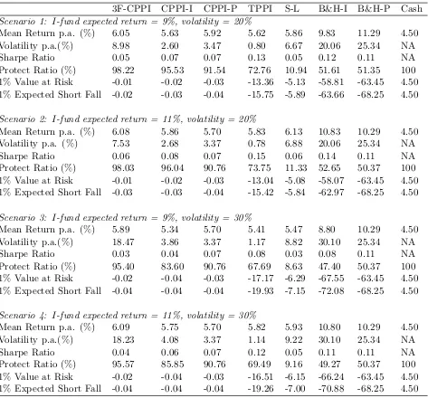
Table 3: This table presents Monte Carlo simulation results of performance measures (e.g. Mean return, volatility, Sharpe ratio etc.) for the proposed 3F-CPPI strategy and other benchmark strategies like CPPI, TPPI among others. The P-fund is fixed with a mean return and volatility of 10% and 25% respectively.
3F-CPPI CPPI-I CPPI-P TPPI S-L B&H-I B&H-P Cash
Scenario 1: I-fund expected return = 9%, volatility = 20%
Mean Return p.a. (%) 6.05 5.63 5.92 5.62 5.86 9.83 11.29 4.50
Volatility p.a.(%) 8.98 2.60 3.47 0.80 6.67 20.06 25.34 NA
Sharpe Ratio 0.05 0.07 0.07 0.13 0.05 0.12 0.11 NA
Protect Ratio (%) 98.22 95.53 91.54 72.76 10.94 51.61 51.35 100
1% Value at Risk -0.01 -0.02 -0.03 -13.36 -5.13 -58.81 -63.45 4.50
1% Expected Short Fall -0.02 -0.03 -0.04 -15.75 -5.89 -63.66 -68.25 4.50
Scenario 2: I-fund expected return = 11%, volatility = 20%
Mean Return p.a. (%) 6.08 5.86 5.70 5.83 6.13 10.83 10.29 4.50
Volatility p.a. (%) 7.53 2.68 3.37 0.78 6.88 20.06 25.34 NA
Sharpe Ratio 0.06 0.08 0.07 0.15 0.06 0.14 0.11 NA
Protect Ratio (%) 98.03 96.04 90.76 73.75 11.33 52.65 50.37 100
1% Value at Risk -0.01 -0.02 -0.03 -13.04 -5.08 -58.07 -63.45 4.50
1% Expected Short Fall -0.03 -0.03 -0.04 -15.42 -5.84 -62.97 -68.25 4.50
Scenario 3: I-fund expected return = 9%, volatility = 30%
Mean Return p.a. (%) 5.89 5.34 5.70 5.41 5.47 8.80 10.29 4.50
Volatility p.a.(%) 18.47 3.86 3.37 1.17 8.82 30.10 25.34 NA
Sharpe Ratio 0.03 0.04 0.07 0.08 0.03 0.08 0.11 NA
Protect Ratio (%) 95.40 83.60 90.76 67.69 8.63 47.40 50.37 100
1% Value at Risk -0.02 -0.04 -0.03 -17.17 -6.29 -67.55 -63.45 4.50
1% Expected Short Fall -0.04 -0.04 -0.04 -19.93 -7.15 -72.08 -68.25 4.50
Scenario 4: I-fund expected return = 11%, volatility = 30%
Mean Return p.a. (%) 6.09 5.75 5.70 5.82 5.93 10.80 10.29 4.50
Volatility p.a.(%) 18.23 4.08 3.37 1.14 9.22 30.10 25.34 NA
Sharpe Ratio 0.04 0.06 0.07 0.12 0.05 0.11 0.11 NA
Protect Ratio (%) 95.57 85.85 90.76 69.49 9.16 49.27 50.37 100
1% Value at Risk -0.02 -0.04 -0.03 -16.51 -6.15 -66.24 -63.45 4.50
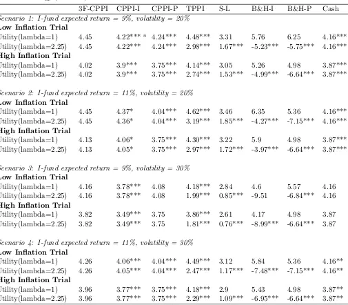
Table 4: This table reports Monte Carlo simulation results of the utility value for loss averse investors under two inflation levels. The P-fund is fixed with a mean return and volatility of 10% and 25% respectively. The null hypothesis in the paired t-test is that the loss averse utility of a portfolio insurance strategy is equal to that of the best corresponding benchmark strategy (3F-CPPI).
3F-CPPI CPPI-I CPPI-P TPPI S-L B&H-I B&H-P Cash
Scenario 1: I-fund expected return = 9%, volatility = 20%
Low Inflation Trial
Utility(lambda=1) 4.45 4.22***a 4.24*** 4.48*** 3.31 5.76 6.25 4.16***
Utility(lambda=2.25) 4.45 4.22*** 4.24*** 2.98*** 1.67*** -5.23*** -5.75*** 4.16***
High Inflation Trial
Utility(lambda=1) 4.02 3.9*** 3.75*** 4.14*** 3.05 5.26 4.98 3.87***
Utility(lambda=2.25) 4.02 3.9*** 3.75*** 2.74*** 1.53*** -4.99*** -6.64*** 3.87***
Scenario 2: I-fund expected return = 11%, volatility = 20%
Low Inflation Trial
Utility(lambda=1) 4.45 4.37* 4.04*** 4.62*** 3.46 6.35 5.36 4.16***
Utility(lambda=2.25) 4.45 4.36* 4.04*** 3.19*** 1.85*** -4.27*** -7.15*** 4.16***
High Inflation Trial
Utility(lambda=1) 4.13 4.06* 3.75*** 4.30*** 3.22 5.9 4.98 3.87***
Utility(lambda=2.25) 4.13 4.05* 3.75*** 2.97*** 1.72*** -3.97*** -6.64*** 3.87***
Scenario 3: I-fund expected return = 9%, volatility = 30%
Low Inflation Trial
Utility(lambda=1) 4.16 3.78*** 4.08 4.18*** 2.84 4.6 5.57 4.16
Utility(lambda=2.25) 4.16 3.78*** 4.08 1.99*** 0.85*** -9.51 -6.84*** 4.16
High Inflation Trial
Utility(lambda=1) 3.82 3.49*** 3.75 3.86*** 2.61 4.17 4.98 3.87
Utility(lambda=2.25) 3.82 3.49*** 3.75 1.81*** 0.76*** -8.99*** -6.64*** 3.87
Scenario 4: I-fund expected return = 11%, volatility = 30%
Low Inflation Trial
Utility(lambda=1) 4.26 4.06*** 4.04*** 4.49*** 3.12 5.84 5.36 4.16**
Utility(lambda=2.25) 4.26 4.05*** 4.04*** 2.47*** 1.17*** -7.48*** -7.15*** 4.16**
High Inflation Trial
Utility(lambda=1) 3.96 3.77*** 3.75*** 4.18*** 2.9 5.43 4.98 3.87**
Utility(lambda=2.25) 3.96 3.77*** 3.75*** 2.29*** 1.09*** -6.95*** -6.64*** 3.87**
a The test statistic is significant at the 10% level; **The test statistic is significant at the 5% level; ***The
4.3.1. Investor utility
Overall, the simulation results show that 3F-CPPI significantly outperforms other benchmark strategies regardless of investors’ utility functions.
In the non-loss-averse case with λ= 1, 3F-CPPI dominates all the benchmark strate-gies except TIPP and B&H. Almost in all four scenarios, TIPP and B&H exhibits higher utility value for non-loss-averse SPGFs investors. However, it is not significantly higher than 3F-CPPI according to the t-test.
While in the loss averse withλ= 2.25, 3F-CPPI dominates almost all strategies in the total eight scenarios of two trails. More specifically, in Scenario 1 of Table 4, the 3F-CPPI exhibits the highest prospect utility in the case of loss averse across all the strategies, with a value of 4.45. Moreover, 3F-CPPI is more favoured by SPGFs investors with higher loss averse utility. This is because for higher risk averse investors, there is almost no reduction of utility for 3F-CPPI strategy while other strategies experience drastically fall of utility value. For instance, TIPP, stop-loss and especially B&H-P strategies experience a big fall (from 6.25 to -5.75) as the increase of loss averse parameter λ from 1 to 2.25.
4.3.2. Downside risk protection
Sustaining a guaranteed return and preventing loss are the main purposes of a port-folio insurance strategy. In both trials, 3F-CPPI reveals the superiority of managing the downside risk. Our numerical results indicate that 3F-CPPI dominates almost all the other strategies except the cash investment in term of the protect ratio, 1% value at risk and 1% expected shortfall.
As can be seen in the Scenario 1 of Table 3, the 1% value at risk of 3F-CPPI is -0.01 %, much higher than TIPP (-13.36 %), S-L (-5.13 %), and B&H-P (-63.45 %). 3F-CPPI also has the highest 1% expected shortfall and the protection ratio as well compared with other benchmark strategies. Overall 3F-CPPI proves to be a competent strategy with regard to preventing downward return and sustaining guaranteed return.
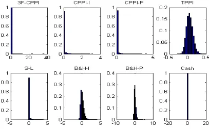
Also, as indicated in Figure 5, 3F-CPPI’s return distribution achieves a higher protec-tion ratio and with upside potential as well. Unlike B&H and TPPI, 3F-CPPI controls the downside risk as well.
4.3.3. 3F-CPPI versus CPPI
Figure 5: The return distributions of all strategies in the Scenario 1
Moreover, 3F-CPPI outperforms CPPI in preventing downside risk. For example, in Scenario 1 of Table 4, CPPI-P has only a protection ratio value of 91.54% while 3F-CPPI has a much higher value of 98.22%. The superiority of 3F-3F-CPPI also holds in other measures such as 1% value at risk. Overall 3F-CPPI has proven to be a competent strategy with higher return and volatility as well as a better downside risk protection.
4.3.4. Market condition effect
Although 3F-CPPI dominates other strategies in almost all scenarios, the superior-ity has been mainly affected by market conditions, i.e. the relativsuperior-ity between I-fund and P-fund. In particular, 3F-CPPI loses its advantages when the stock market I-fund outperforms the purpose-related market sector P-fund. The reason is straightforward as 3F-CPPI invests in an extra third fundP-fund to hedge the purpose-related inflation risk.
5. Conclusion
Loss averse investors, especially pensioners, has an increasingly high demand for hedg-ing special purpose risks like medical and education costs. Although there are various types of funds promising a minimum guaranteed return plus a common specific use of the investment like pension, the investment strategies adopted is way out of optimal. There-fore, an innovative 3F-CPPI strategy has been constructed in this paper with the aim of improving the performance of SPGF for loss averse investors.
Overall, the proposed 3F-CPPI outperforms other strategies in terms of hedging against the downside risk and satisfying the investors’ utility. We first derive explicit optimal allocations for 3F-CPPI and discuss further the relationship between the optimal proportion of purpose-related fund and leverage ratio. Generally the optimal proportion of purpose-related fund mainly depends on the performance relativity of stock index and purpose-related fund.
We theoretically prove that the proposed 3F-CPPI dominates CPPI in both the dis-crete and continuous time cases, followed by extensive Monte Carlo simulation checking the practicability of 3F-CPPI. Theoretical analysis shows that the investment in a third fund to hedge purpose-related risk contributes to 3F-CPPI’s superior performance and higher investor utility. Under the discrete time case with gap risk, the Monte Carlo sim-ulation has been adopted for performance comparison among the proposed 3F-CPPI and other benchmark strategies, including CPPI, TIPP, stop-loss and B&H. The numerical analysis illustrates that 3F-CPPI demonstrates in achieving relatively higher mean re-turn, better portfolio protection and higher investor’s prospect utility as well. Moreover, our findings claim that the advantage of 3F-CPPI increases with loss aversion, indicating that 3F-CPPI is much more preferred to the standard CPPI and other strategies for loss averse investors.
In summary, this paper proposed an applicable modified CPPI strategy, 3F-CPPI, within a general portfolio insurance setting. both theoretical and practical insights. 3F-CPPI dominates other strategies in many aspects such as the protection ratio, downside risk and loss averse utility. In this paper we apply only the three fund allocation rule to standard CPPI strategy, while, it is worthwhile to extend it to other portfolio insurance strategies, which we leave for future research.
Acknowledgements
Appendices
Appendix A Proof of Propositions
A.1 Proof of Proposition 1
Proof: The stochastic process of a 3F-CPPI portfolio value at time t follows
dVt=Et[α
dSI
t
SI
t
+ (1−α)dS
P t
SP
t
] + (Vt−Et)rdt (A.1)
=mCt{[α(µi−r) + (1−α)(µp−r)dt+ασidZs+ (1−α)σpdZP}+rVtdt. (A.2)
Denote risk premium of I-fund and P-fund by
θi =
µi−r
σi
, θP =
µp−r
σP
, (A.3)
respectively. (A.1) can be simplified to
dVt =rPtdt+Ct{r+m[ασiθi+ (1−α)σPθP]}dt+mCt[ασidZs+ (1−α)σPdZP].
Define stochastic process Bt as follows, with B0 = 0 :
dBt={r+m[ασiθi+ (1−α)σPθP]}dt+m[ασidZs+ (1−α)σPdZP], (A.4)
Bt={r+m[ασiθi+ (1−α)σPθP]}t+m[ασiWst + (1−α)σPW pt], t ∈[0, T].
Then, Vt is driven by Bt,
dVt=rPtdt+CtdBt. (A.5)
By (A.4) the dBtdBt is
dBtdBt= [m2α2σ2i +m
2
(1−α)2σP2 + 2m2α(1−α)ρsPσiσp]dt. (A.6)
For simplification, denote
A=m2α2σi2+m2(1−α)2σ2P + 2m2α(1−α)ρsPσiσp. (A.7)
Then, consider an exponential process f(Z):
f(Bt) = exp(−Bt+
1
2At). (A.8)
By Ito’s lemma:
df(Bt) =−f(Bt)dBt+
1
2Af(Bt)dt+ 1
2f(Bt)dBtdBt
By (A.5),
dVt=dCt+dPt
=dCt+dPtdt
=rPtdt+CtdBt, (A.10)
we have:
dCt=CtdBt+ (r−d)Ptdt. (A.11)
Thus, consider the SDE process of the Ctf(Bt):
d[Ctf(Bt)] =f(Bt)dCt+Ctdf(Bt) +dCtdf(Bt)
=f(Bt)[CtdBt+ (r−d)Ptdt] +Ct[−f(Bt)dBt+Af(Bt)dt]−Ctf(Bt)Adt
=f(Bt)(r−d)Ptdt, t∈[0, T]. (A.12)
Due to f(B0) = 1, we have:
Ctf(Bt) =C0+ (r−d)
Z t
0
f(Bξ)Pξdξ,
Vt =Pt+C0exp(Bt−
1
2At) + (r−d)
Z t
0
exp{Bt−Bξ−
1
2A(t−ξ)}Pξdξ. (A.13)
As for the expected value of a 3F-CPPI portfolio at time t is:
E(Vt) = Pt+C0eµBt+ (r−d)p0eµBt
1−e(d−µB)t
µB−d
, (A.14)
as Vt is in the (A.13):
Vt =Pt+C0exp(Bt−
1
2At) + (r−d)
Z t
0
exp{Bt−Bξ−
1
2A(t−ξ)}Pξdξ. (A.15)
By property of log-normal distribution, expectation of exp(Bt−12At) is:
E{exp(Bt−
1
2At)}= exp(− 1
2At)E{exp(Bt)} (A.16)
= exp(−1
2At) exp(µBt+ 1 2At) = exp(µBt).
Then,
E(Vt) = Pt+eµBt{C0+ (r−d)E[
Z t
0
exp(−Bξ+
1
Fubini-Tonelli theorem ensures that taking the expectation it becomes:
E(Vt) =Pt+eµBt{C0+ (r−d)E[
Z t
0
exp(−Bξ+
1
2Aξ)Pξdξ]}
=Pt+eµBt{C0+ (r−d)P0
Z t
0
E[exp(−Bξ+
1
2Aξ)Pξ]dξ}
=Pt+eµBt{C0+ (r−d)P0
1−e(d−µB)t
µB−d
}. (A.18)
Therefore, for anyt ∈[0, T], we can have:
E(Vt) =Pt+eµBt{C0+ (r−d)P0eµBt
1−e(d−µB)t
µB−d
}. (A.19)
A.2 Proof of Proposition 2
Proof: Consider a representative investor with risk averse attitudeγ <1, the maximiza-tion problem with utility in (10) is equivalent to:
M ax
m,α {−
1
2A−µY +r+m(ασ
s
iθi+ (1−α)σpθp) (A.20)
+γ
2[(mασ
s
i +m(1−α)σ s p −σ
i y)
2
+ (m(1−α)σpp−σyp)2+ (σye)2]}. (A.21)
If we consider the most common the fixed-rate floor strategy r = d case, the opti-mization problem is equivalent to
M ax
m,α µx+
1
2(γ−1)σ 2
x, (A.22)
where σx2 = [mασi +m(1−α)σps− σiy]2 + [m(1−α)σpp −σyp]2 + (σye)2. Therefore, the
maximization function (A.22) punishes for investment volatility as the investors’ γ is less than 1, withRRA = 1−γ >0.
M ax
m,α E[U(VT, YT|F0) (A.23)
= M ax
m,α E[u(
RT
YT
) +v(VT −RT
YT
)|F0] (A.24)
⇐⇒ M ax
m,α E[v(
VT −RT
YT
)|F0] (A.25)
= M ax
m,α E[(
VT −RT
YT
)γ] (A.26)
As stated earlier, a typical reference point RT is the SPGF guaranteed amountPT, thus
u(RT
Consider the representative investors’ risk averse attitude is γ <1, denote
xt = (Vt−Pt)/Yt=Ct/Yt.
xtindicates 3F-CPPI portfolio’s deviation compared to reference at timet. By the explicit
form ofCt and Yt, we have
xt=
C0exp(Bt−12At) + (r−d)
Rt
0 exp{Bt−Bξ− 1
2A(t−ξ)}Pξdξ exp(µYt+σYWY t)
. (A.27)
If we further assume the fixed-rate floor case with r=d, (A.27) is simplified into:
xt =C0exp(Bt−
1
2At−µYt−σYWY t)
=C0exp(− 1
2At−µYt) exp(Bt−σYWY t),
then,
E[1
γ(xt)
γ] = C γ
0
γ exp(−
1
2γAt−γµYt)E[exp(Bt−σYWY t)]
= C
γ
0
γ exp{−
1
2γAt−γµYt+γ[r+m(ασ
s
iθi+ (1−α)σpθp)]t}
exp{γ
2
2[(mασ
s
i +m(1−α)σ s p −σ
i y)
2
+ (m(1−α)σpp−σyp)2+ (σye)2]t}. (A.28)
Hence, the maximization problem in (10) is equivalent to:
M ax
m,α {−
1
2A−µY +r+m(ασ
s
iθi+ (1−α)σpθp) (A.29)
+γ
2[(mασ
s
i +m(1−α)σps−σyi)2+ (m(1−α)σpp−σyp)2+ (σye)2]}. (A.30)
(A.29) can also be deduced by Ito’s lemma. In the fixed-rate floor r=d case,
dCt =CtdBt, (A.31)
and
dYt=µYdt+σYdZY, (A.32)
by ito’s lemma,
dx
x =µxdt+σxdZx, (A.33)
where
µx=r−µY+σY2 +m[ασ
s
iθi+(1−α)σPθP]−m[ασisσ i
y+(1−α)σ s pσ
i
y+(1−α)σ p pσ
p
y], (A.34)
and
σxdZx = [mασsi +m(1−α)σ
s p−σ
i
y]dZs+ [m(1−α)σpp−σ p
Thus,
E(xγ) = exp{[γµx+
1
2γ(γ−1)σ 2
x]t}. (A.35)
the optimization problem is equivalent to
M ax
m,α µx+
1
2(γ−1)σ 2
x, (A.36)
whereσ2
x = [mασi+m(1−α)σps−σsy]2+ [m(1−α)σpp−σyp]2+ (σye)2. It’s noteworthy that
when γ = 0, the utility v(xt) = log(xt), the equivalent maximization form (A.36) still
holds, asE[U(xt)] equals to E[log(xt)] = µx− 12σx2 for the case γ = 0.
Another poof to get (A.36) is by the Ito’s lemma. The optimization problem is:
M ax
m,α E[U(VT, YT|F0) (A.37)
= M ax
m,α E[U(
VT −PT
YT
)|F0], (A.38)
wherePT is the SPGF guaranteed amount. Consider a representative investor with a risk
averse attitude γ <1, then denote
xt = (Vt−Pt)/Yt=Ct/Yt.
xt indicates 3F-CPPI portfolio’s deviation at time t. By the explicit form of Ct and Yt,
we have
xt=
C0exp(Bt−12At) + (r−d)
Rt
0 exp{Bt−Bξ− 1
2A(t−ξ)}Pξdξ exp(µYt+σYWY t)
. (A.39)
If we further assume the fixed-rate floor case with r=d, (A.39) is simplified into:
xt =C0exp(Bt−
1
2At−µYt−σYWY t)
=C0exp(− 1
2At−µYt) exp(Bt−σYWY t),
then,
E[1
γ(xt)
γ
] = C
γ
0
γ exp(−
1
2γAt−γµYt)E[exp(Bt−σYWY t)]
= C
γ
0
γ exp{−
1
2γAt−γµYt+γ[r+m(ασ
s
iθi+ (1−α)σpθp)]t}
exp{γ
2
2[(mασ
s
i +m(1−α)σ s p −σ
s y)
2+ (m(1−α)σp p −σ
p y)
2+ (σe y)
2]t}. (A.40)
Hence, the maximization problem is equivalent to:
M ax
m,α {−
1
2A−µY +r+m(ασ
s
iθi+ (1−α)σpθp) (A.41)
+γ
2[(mασ
s
i +m(1−α)σ s p −σ
i y)
2
(A.41) can also be deduced by Ito’s lemma. In the fixed-rate floor r =d case,
dCt =CtdBt, (A.43)
and
dYt=µYdt+σYdZY, (A.44)
by ito’s lemma,
dx
x =µxdt+σxdZx, (A.45)
where
µx=r−µY+σY2 +m[ασ
s
iθi+(1−α)σPθP]−m[ασisσ s
y+(1−α)σ s pσ
s
y+(1−α)σ p pσ
p
y], (A.46)
and
σxdZx = [mασsi +m(1−α)σ
s p−σ
s
y]dZs+ [m(1−α)σpp−σ p
y]dZp+σeydZe.
Thus,
E(xγ) = exp{[γµx+
1
2γ(γ−1)σ 2
x]t}. (A.47)
the optimization problem is equivalent to
M ax
m,α µx+
1
2(γ−1)σ 2
x, (A.48)
whereσ2
x = [mασi+m(1−α)σps−σsy]2+ [m(1−α)σpp−σyp]2+ (σye)2. It’s noteworthy that
when γ = 0, the utility v(xt) = log(xt), the equivalent maximization form (A.48) still
holds, asE[U(xt)] equals to E[log(xt)] = µx− 12σx2 for the case γ = 0.
Then, we consider the first order conditions (FOCs) for the problem (A.36) are as follows:
αµ(iγ)+(1−α)µ(pγ)−r+(γ−1){[mασi+m(1−α)σsp−σys][ασis+(1−α)σsp]+[m(1−α)σpp−σpy](1−α)σpp}= 0, (A.49)
(µ(iγ)−µ(pγ))+(γ−1){[mασsi+m(1−α)σps−σys](σis−σps)−[m(1−α)σpp−σyp]σpp}= 0. (A.50)
The optimalm∗ and α∗ is straightforward by solving the FOC equations, we get
α∗(m∗)µi(γ)+ (1−α∗(m∗))µp(γ)−r+ (µ(iγ)−µ(pγ))α∗(m∗) (A.51)
+ (γ−1){[(σ
s
p)2+ (σpp)2−σpsσis
(σs
i −σsp)2+ (σ p p)2
+ (σpp)2+ (σps)2]m∗ −σyiσps−σypσpp}= 0,
α∗(m) = (σ
s
p)2+ (σpp)2−σpsσis
(σs
i −σsp)2+ (σ p p)2
+ µ
(γ)
i −µ
(γ)
p
(σi−σsp)2+ (σ p p)2
1
To solve the expressions of m∗ and α∗, in the following we denote some terms by D, E, F
for simplicity,
D= (γ−1)·[(σ
s
p)2 + (σpp)2−σspσis
(σs
i −σps)2+ (σ p p)2
+ (σpp)2+ (σsp)2],
E = 2(µ(iγ)−µp(γ))·[(σ
s
p)2+ (σpp)2−σpsσsi
(σs
i −σsp)2+ (σ p p)2
+µ(pγ)−r−(γ−1)(σysσsp+σypσpp)],
F = (µ
(γ)
i −µ
(γ)
p )2
(σs
i −σps)2+ (σ p p)2
· 2
1−γ.
The m∗ is the solution of the following quadratic equation:
Dm2+Em+F = 0.
It is easy to find out that in most cases, the solution ism∗ = max(−E+ √
E2−4DF 2D ,
−E−√E2−4DF 2D ),
then α∗ = (σsp)2+(σ p p)2−σspσsi
(σs
i−σps)2+(σpp)2 +
µ(iγ)−µ(pγ)
(σi−σps)2+(σpp)2
1 (1−γ)m∗.
References
Apergis, N. and Miller, S. M. (2009), ‘Do structural oil-market shocks affect stock prices?’, Energy Economics31(4), 569–575.
Arnott, R. D. and Bernstein, P. L. (2002), ‘What risk premium is normal?’, Financial Analysts Journal 58(2), 64–85.
Bahram, A., Arjun, C. and Kambiz, R. (2004), ‘Reit investments and hedging against inflation’, Journal of Real Estate Portfolio Management 10(2), 97–112.
Balder, S., Brandl, M. and Mahayni, A. (2009), ‘Effectiveness of cppi strategies under discrete-time trading’,Journal of Economic Dynamics and Control 33(1), 204–220.
Benartzi, S. and Thaler, R. H. (1995), ‘Myopic loss aversion and the equity premium puzzle’,The quarterly journal of Economics 110(1), 73–92.
Benninga, S. (1990), ‘Comparing portfolio insurance strategies’, Finanzmarkt und Port-folio Management 4(1), 20–30.
Black, F. and Jones, R. W. (1987), ‘Simplifying portfolio insurance’, The Journal of Portfolio Management 14(1), 48–51.
Black, F. and Perold, A. (1992), ‘Theory of constant proportion portfolio insurance’, Journal of Economic Dynamics and Control 16(3-4), 403–426.
Boyd, J. H., Levine, R. and Smith, B. D. (2001), ‘The impact of inflation on financial sector performance’, Journal of Monetary Economics47(2), 221–248.
Cairns, A. J., Blake, D. and Dowd, K. (2006), ‘Stochastic lifestyling: Optimal dynamic asset allocation for defined contribution pension plans’,Journal of Economic Dynamics and Control 30(5), 843–877.
Chen, J.-S., Chang, C.-L., Hou, J.-L. and Lin, Y.-T. (2008), ‘Dynamic proportion port-folio insurance using genetic programming with principal component analysis’, Expert Systems with Applications35(1), 273–278.
Dahlquist, M., Farago, A. and T´edongap, R. (2016), ‘Asymmetries and portfolio choice’, The Review of Financial Studies 30(2), 667–702.
Dichtl, H. and Drobetz, W. (2011), ‘Portfolio insurance and prospect theory investors: Popularity and optimal design of capital protected financial products’,Journal of Bank-ing & Finance35(7), 1683–1697.
Dimson, E., Marsh, P. and Staunton, M. (2008), The worldwide equity premium: a smaller puzzle,in ‘Handbook of the equity risk premium’, Elsevier, pp. 467–514.
Dybvig, P. and Liu, F. (2018), ‘On investor preferences and mutual fund separation’, Journal of Economic Theory174, 224–260.
Estep, T. and Kritzman, M. (1988), ‘Tipp: Insurance without complexity’, The Journal of Portfolio Management14(4), 38–42.
Figlewski, S., Chidambaran, N. and Kaplan, S. (1993), ‘Evaluating the performance of the protective put strategy’, Financial Analysts Journalpp. 46–69.
Hakansson, N. H. (1969), ‘Risk disposition and the separation property in portfolio selec-tion’,Journal of Financial and Quantitative Analysis 4(4), 401–416.
Herold, U., Maurer, R. and Purschaker, N. (2005), ‘Total return fixed-income portfolio management’,The Journal of Portfolio Management 31(3), 32–43.
Hoesli, M. and Oikarinen, E. (2012), ‘Are reits real estate? evidence from international sector level data’,Journal of International Money and Finance 31(7), 1823–1850.
Huu Do, B. (2002), ‘Relative performance of dynamic portfolio insurance strategies: Aus-tralian evidence’, Accounting & Finance42(3), 279–296.
Kang, W., Ratti, R. A. and Yoon, K. H. (2015), ‘The impact of oil price shocks on the stock market return and volatility relationship’,Journal of International Financial Markets, Institutions and Money34, 41–54.
Markowitz, H. (1959), ‘Portfolio selection, cowles foundation monograph no. 16’, John Wiley, New York. S. Moss (1981). An Economic theory of Business Strategy, Halstead Press, New York. TH Naylor (1966). The theory of the firm: a comparison of marginal analysis and linear programming. Southern Economic Journal (January)32, 263–74.
Merton, R. C. (1973), ‘Theory of rational option pricing’, The Bell Journal of economics and management sciencepp. 141–183.
Pye, G. (1967), ‘Portfolio selection and security prices’, The Review of Economic and Statistics pp. 111–115.
Ross, S. A. (1978), ‘Mutual fund separation in nancial theory: The separating distribu-tions’,Journal of Economic Theory pp. 254–286.
Rubens, J., Bond, M. and Webb, J. (1989), ‘The inflation-hedging effectiveness of real estate’,Journal of Real Estate Research 4(2), 45–55.
Sadorsky, P. (2001), ‘Risk factors in stock returns of canadian oil and gas companies’, Energy economics 23(1), 17–28.
Samuelson, P. A. (1967), ‘General proof that diversification pays’, Journal of Financial and Quantitative Analysis2(1), 1–13.
Tobin, J. (1958), ‘Liquidity preference as behavior towards risk’, The review of economic studies25(2), 65–86.