Modelling Socio-Economic Differences in Mortality Using a New Affluence Index

City, University of London Institutional Repository

Citation

:

This is the accepted version of the paper.

This version of the publication may differ from the final published

version.

Permanent repository link:

Link to published version

:

Copyright and reuse:

City Research Online aims to make research

outputs of City, University of London available to a wider audience.

Copyright and Moral Rights remain with the author(s) and/or copyright

holders. URLs from City Research Online may be freely distributed and

linked to.

City Research Online: http://openaccess.city.ac.uk/ [email protected]

By

Andrew J.G. Cairns, Malene Kallestrup-Lamb, Carsten P.T. Rosenskjold, David Blake and Kevin Dowda

Abstract

We introduce a new modelling framework to explain socio-economic differences in mortality in terms of an affluence index that combines information on individual wealth and income. The model is illustrated using data on older Danish males over the period 1985-2012 reported in the Statistics Denmark national register database. The model fits the historical mortality data well, captures their key features, gener-ates smoothed death rgener-ates that allow us to work with a larger number of sub-groups than has previously been considered feasible, and has plausible projection properties.

Keywords: Affluence index; Danish mortality data; CBD-X model; gravity model; multi-population mortality modelling; forward correlation term structure.

JEL codes: J11, C53, G22

a_{Andrew Cairns: Maxwell Institute for Mathematical Sciences, Edinburgh, and Department}

of Actuarial Mathematics and Statistics, Heriot-Watt University, Edinburgh, EH14 4AS, UK.

E-mail: [email protected]. Malene Kallestrup-Lamb and Carsten Rosenskjold: Center for

Research in Econometric Analysis of Time Series (CREATES), Department of Economics and

Business Economics, Aarhus University, Fuglesangs All´e 4, DK-8210 Aarhus V, Denmark. E-mail:

1

Introduction

There has been increasing interest in recent years in explaining and projecting mor-tality in closely related populations, such as those of neighbouring countries or sub-groups of a national population for which there is sufficient heterogeneity in the mortality experience of the sub-groups to justify modelling them separately. Multi-population stochastic mortality models have been developed which help us under-stand historical differences in the mortality of different populations and ensure that we obtain plausible projections of mortality improvements. Such projections will satisfy the following five criteria:

• Generate a projected trend that is consistent with the historical trend in mor-tality improvements.

• Produce levels of variability consistent with that observed in the historical data.

• Preserve sub-group rankings, where these seem justified.

• Generate coherent projections across sub-groups, discussed in more detail be-low.

• Produce plausible forward correlations between sub-groups over different ages and future horizons (see Appendix A for a definition and analysis of forward correlations).

For discussion of these criteria, see Hyndman et al. (2013), Villegas et al. (2017) and the references therein.

A key problem that is frequently encountered is that some of the populations of interest can be quite small and hence involve significant sampling variation. In some cases, it is possible to circumvent this problem by using the mortality experience of a larger (e.g., the national) population to help inform and improve projections of the smaller (e.g., a sub-) population of interest. To illustrate, the mortality experience in an annuity provider’s book of business can be modelled jointly with that of the national population. For examples, see Coughlan et al. (2011), Villegas et al. (2017), and Cairns and El Boukfaoui (2017). In other cases, we might be interested in subdividing the national population into a large number of smaller populations on the basis of certain criteria. A prominent current example is socio-economic differences in mortality experience. The challenge is to extract underlying death rates from the noisy sub-population data.

Our paper addresses this challenge. Specifically, we wish to:

consistent degree of heterogeneity in those mortality rates (i.e., maintains a consistent ranking of mortality rates) on the basis of the selected criteria.

• Develop a stochastic multi-population mortality model that fits the data well.

• Use Bayesian estimation methods to dampen the impact of sampling variation in the sub-group data.

• Use the resulting multi-population mortality model to make mortality pro-jections that link sub-group-specific mortality improvements to the national trend through a gravity effect which prevents the former deviating too far from the latter.

Our specific purpose is to model socio-economic differences in mortality. We have ac-cess to a comprehensive national database maintained by Statistics Denmark which allows us to model and project the socio-economic mortality of older Danish males using the above four-part modelling approach. This database also allows us to construct a new affluence index that can be used to divide up the Danish male population into distinct socio-economic sub-groups. We find that this index is a suf-ficiently strong predictor of high or low mortality to allow subdivision of the national population into 10 sub-groups. In addition, the use of Bayesian methods enables us to separate the population into a larger number of sub-groups than would nor-mally be advisable (for a population the size of Denmark) using more conventional likelihood-based techniques common in mortality modelling. The results achieved using the affluence index have greater precision than those using alternative predic-tive variables (or covariates), such as income or wealth alone.

Our approach:

• Fits the historical data well.

• Dampens sampling variation whilst still preserving the main features of the data (e.g., the shape of the underlying mortality curves by age in each group, the gaps between groups at all ages and in all years, and the idiosyncracies of the underlying time trends). In doing so, it also generates a clear ordering (i.e., avoids cross-overs) of the death rates for the 10 deciles at all ages from 55 to 94 and in all years.

socio-economic group has a lower probability of dying than someone of the same age and gender from a lower socio-economic group over the next and subsequent years.

• Produces a plausible forward correlation term structure between the mortality rates of different groups (see Appendix A). Knowledge of this correlation term structure is important in some financial applications where risk management strategies depend on reliable correlation estimates (see Section 6).

It is important to note that our modelling framework does not impose any specific group ordering, since neither the prior distributions nor the likelihood function con-tain any assumption about the ordering of the groups. It therefore follows that, while multiple cross-overs of the different groups are perfectly possible in our frame-work, this would be a sure indication that the affluence index was a poor covariate for discriminating between the different social classes.

The approach has a number of potentially useful applications:

• It allows government agencies to generate more accurate estimates of the cost and projected increases in the cost of state pension benefits in different pop-ulation segments.

• It helps corporate pension plans improve estimates of their liabilities, given information about the socio-economic mix of their plan members.

• It allows annuity providers to price annuities more accurately on a socio-economic basis.

• It allows for the improved design of hedges for mortality-linked financial prod-ucts.

In short, the use of a powerful predictive variable, such as the affluence index, allows life insurers, for example, to identify the different life expectancies of different socio-economic groups more accurately, which, in turn, leads to more reliable risk rating of customers, improved premium setting, more accurate reserving calculations, and more effective hedging.

change around 1995, the mortality and life-expectancy gaps between different groups at different ages, and the changing levels of inequality between groups over time). The section following analyses properties of projected mortality: central trends, uncertainty and correlations between sub-groups. We finish with some applications, extensions and conclusions.

2

Data

2.1

The Statistics Denmark database

The analysis in this paper makes use of a high quality database from Statistics Den-mark (SD), derived from administrative records. Since every individual in DenDen-mark is given a central personal register (CPR) number either at birth or when given residence permission in the country, we are able to uniquely identify each individual across all components of the public register system. For each individual, we have information on their date of birth, education, income, wealth, and, ultimately, their date of death. We can also identify the same information for an individual’s spouse or partner, thereby enabling us to allocate income and wealth within households.

The database also allows us to identify three financial indicators for each individual and couple, all rebased to year 2000 real values: gross individual annual income, total net household income, and net household wealth. All financial measures are derived from calculations made by the tax authorities which are linked to the CPR. See Appendix B for further details.

Data are available for calendar years 1980 to 2012. However, as the quality of both the income and wealth data (especially for married couples) is regarded as less reliable at the beginning of the period, we disregard the first four years of the available data. In addition, since our methodology for allocating individuals into sub-groups requires data for the previous calendar year, we calculate exposures and deaths data for each sub-group for the 1985-2012 period only.

One of the key objectives is to identify variables derived from information available on the SD database that have a strong predictive power in explaining the mortality of different individuals in the population. More specifically, we wish to subdivide the population at each age and in each year into a number, N, of approximately equal-sized sub-groups, with a clear and unchanging ordering between sub-groups in terms of mortality ratesat all ages: that is, Group 1 should ideally have the highest mortality at all ages and GroupN the lowest. From the outset, we aimed for a larger number of sub-groups than has typically been the case in other studies (Brønnum-Hansen and Baadsgaard (2012), for example, subdivide the Danish population into

For a subsample of the US population (over 50 times bigger than Denmark), Wal-dron (2013) is able to achieve statistically meaningful results using deciles based on lifetime earnings covering a more limited range of ages (63-71) than in this paper (55-94). Chetty et al. (2016) report similar results for the US over ages 40-76 using taxable income.

For Denmark, we show that separation into deciles also gives meaningful results, but requires greater effort to filter out or smooth the effects of sampling variation. We also found that the use of deciles revealed weaknesses in some previously considered covariates that would not be so readily apparent if we were to use, say, N = 3 or 4 sub-groups. Extensive experimentation helped not only to identify these weaknesses (see, e.g., Figure 5 below), but also led us to identify a new and, in our view, superior predictive variable, namely affluence with lockdown (i.e., fixing sub-group membership) at a certain age (67 in the case of Danish data).

In this study, we aim to identify a single composite index derived from personal financial data that is a strong predictor of mortality. Our reasons for choosing to focus on financial variables from the outset are twofold. First, income and wealth are well known to be strong predictors of mortality (e.g., Waldron, 2013, Brønnum-Hansen and Baadsgaard, 2012, and Chetty et al., 2016). Second, we seek to develop a modelling framework that could be applied to other countries and sub-populations where some measure of income and/or wealth is available.

The candidate covariates considered were income, individual wealth, household wealth, and, as discussed below, linear combinations of these.

2.2

The affluence index: construction and allocation of

in-dividuals to sub-groups

In this section, we show how the affluence index is constructed and then how it is used to allocate individuals to sub-groups.

The affluence index,A(i, t, x), for individuali, in year t at agex (at the start of the year) is defined as the individual’s wealth plusK times their income in the preceding year, that is:

A(i, t, x) =W(i, t−1, x−1) +K×Y(i, t−1, x−1) (1)

where W(i, t−1, x−1) is the (physical and financial) net wealth for individual i, at agex−1 in year t−1 and Y(i, t−1, x−1) is the income of individuali, at age

x−1 in year t−1. K is a constant across the whole population. We interpretK as a capitalisation factor for retirement income. We chose K = 15 to reflect the idea that, around the age of retirement, 15×income is a rough estimate of the present value of an individual’s future retirement income. This follows because, in a low interest-rate environment, K is approximately equal to national life expectancy at retirement age (see Figure 2). Although income and wealth are highly correlated, we found that the variables combine to create a more effective index that produces consistent results between all 10 groups across all years and ages.

Representative values for the affluence index are given in Table 1 for ages 55 and 65 in 1990 and 2010. The values shown are the boundaries between adjacent groups. From Table 1 we can see that: in real terms, there has been modest growth in affluence (0.5% to 1% per annum depending on age and group); and, in relative terms, there has been a slight widening of the gap between Groups 1 and 10 (0.3% to 0.4% per annum).

Individuals not resident in Denmark for the entirety of the previous year are excluded (a small proportion – about 5% – of the full population). The affluence index is then used to allocate all remaining individuals to specific sub-groups. Based on the value of the index,A(i, t, x), each individual, i, in yeartat age xis ranked from 1,2, ..., n, wheren is the number of individuals at age xin year t. The rank of the individuals is given byR(i, t, x). This rank is normalised byU(i, t, x) =R(i, t, x)/(n+ 1), so it is evenly spread between 0 and 1. Then, if U(i, t, x) lies between 0 and 1/10, the individual is allocated to Group 1, and so on. This procedure implies that 10% of the total population is assigned to each sub-group, based on data that are available at the start of the year. Individuals can therefore transition between affluence sub-groups over time (until an individual reaches age 67). These transitions could be modelled formally using a multi-state model (see, e.g., Kwon and Jones, 2008). We comment briefly on the potential impact of these transitions in Section 2.3, but leave a formal analysis of this for future work.

Year: 1990 Year: 2010 Group Boundary Age 55 Age 65 Age 55 Age 65

1→2 2324 1803 2521 2026

2→3 3141 2184 3492 2451

3→4 3588 2518 4056 2898

4→5 3970 2842 4542 3354

5→6 4361 3218 5038 3866

6→7 4836 3655 5568 4474

7→8 5428 4219 6245 5224

8→9 6335 5094 7261 6317

9→10 8139 6855 9421 8356

Table 1: Boundaries (in ’000s of Danish krone) between the 10 affluence groups for ages 55 and 65 and in years 1990 and 2010; e.g., individuals aged 65 on 1 January 2010 will be assigned to affluence Group 3 if their affluence index for 2009 lies between 2,451,000 DKK and 2,898,000 DKK. Amounts are rebased to year 2000 values. 1000DKK≈156USD (31/10/2017).

their 67th year, the main state pension age for most of the period. (The state pension age was reduced from 67 in 2004 to 65, although it will increase to 67 between 2024 and 2027, with further increases after 2027 linked to increases in life expectancy.) From age 67 onwards, each individual is assumed to remain in the same sub-group that they were allocated to at age 66. We call this procedure lockdown.

There are two key benefits arising from this procedure. First, we found that the use of the affluence index is a more effective covariate across all ages (from 55 to 94) and in all years than income or wealth on their own. Second, lockdown at age 67 produces much better results (including improved separation between the 10 sub-groups) than not locking down and allowing transitions between groups after age 67. An additional advantage of lockdown is that it restricts the potential for Group 1 to fill up after age 67 with individuals in severely declining health who have used up most of their personal savings on long-term care. Allowing for such transitions would artificially inflate Group 1 mortality at high ages and depress it in the more affluent sub-groups.

Despite these benefits of using lockdown, the following counterpoints are worth considering:

differences between the 10 mortality curves and, in particular, preserving into higher ages the rankings that we observe at age 67: we are much less interested in theabsolute differences between groups.

• Since affluence is a good predictor of future mortality, lockdown at 67 disre-gards potentially valuable predictive information on affluence at higher ages. To illustrate, individuals age 70 who have used up all personal savings could subsequently experience mortality rates closer to those of Group 1 than those of whatever group they were in at age 67. While accepting such possibilities, we provide a couple of cases where lockdown at, say, 67 is necessary. The first is where we are more interested in, say, the life expectancy of individuals at 67 than single-age mortality rates. Lockdown avoids the problem of individuals changing groups and enables life expectancy to be calculated, assuming the individual stays in the same group. There are many variants of this. Second, from an actuarial perspective, we might wish to price an annuity at the time of retirement. Since we have information about the individual at age 67 only, we need to know what is the typical mortality trajectory of someone with those characteristics at this age and this necessitates the use of lockdown. Further, for reserving, once in payment, an insurance company is unlikely to receive ad-ditional information about the health or affluence of an annuitant until they die – again all it will know is the annuitant’s status at age 67 when the annuity was purchased.

• Lockdown may produce better separation between the sub-groups, but it might be a disadvantage when designing effective hedges for certain mortality-linked products. While it would clearly be useful to be able to recalibrate a hedge in the light of new information, as with the previous point, it depends on whether or not information on those covered by the hedge is updated after they retire.

Finally, we note that the 10 sub-group allocations were not sensitive to the choice ofK, the capitalisation factor for retirement income, in the range 10 to 20. A more sophisticated model would make K a function of age and interest rates. However, the lack of sensitivity of the sub-group allocations to values of K across this wide range suggests that such additional sophistication might not add much – at least in the case of older Danish males – and instead might lead to an unjustified illusion of precision. As a rule of thumb, we suggest thatK could be set approximately equal to the life expectancy at the lockdown age.

2.3

Deaths, exposures and age-specific death rates

50

100

200

500

1000

1500

2000

2500

2500

3000

3500

3500

4000

1985 1995 2005

60

70

80

90

Males: Group 1

Year

Age

50

100

200

500

1000

1500

2000

2500 ₃₀₀₀

3500

3500

4000

1985 1995 2005

60

70

80

90

Males: Group 10

Year

Age

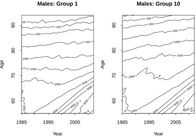
Figure 1: Contour plot of the exposures by year and age for Groups 1 and 10.

• D(i, t, x) = the number of individuals allocated to sub-groupi at the start of the year, born in calendar year t−1−x(i.e., who: (a) are age x at the start of calendar year t or (b) attain their x+ 1th _{birthday during year t) who die}

during calendar year t.

• EI(i, t, x) = the number of individuals allocated to sub-group i, born in

cal-endar year t−1−x, and counted on the first of January in yeart; EI(i, t, x)

is referred to by actuaries as theinitial exposed to risk.

• E(i, t, x) is the corresponding central exposed to risk, and measures the average size of the population during yeartin sub-groupiborn in yeart−1−x. Migra-tion of people into and out of Denmark prevents us from calculatingE(i, t, x) exactly, so we have chosen to use the common approximation E(i, t, x) =

EI(i, t, x)−D(i, t, x)/2.

The age-specific death rate is then

ˆ

m(i, t, x) =D(i, t, x)/E(i, t, x)

Contour plots of the exposures over the period 1985 to 2012 and ages 55 to 94 for Groups 1 and 10 are presented in Figure 1. We can see variation in cohort sizes over time, peaking at age 55 in 2002. By design, the two groups are approximately equal in size up to age 67. Thereafter, due to lockdown, Group 1 exposures decrease at a faster rate than Group 10: at age 94, Group 10 typically has 3 to 4 times the number of members remaining than Group 1.

Exposures, E(i, t, x), range (across all years) from about 4250 (at age 55) down to 13 (at age 94). Deaths, D(i, t, x), range from 151 (peak mortality ages) down to 4 (age 94). It is evident, therefore, that subdividing an already small national population produces crude age-specific death rates that will be subject to quite significant sampling variation.

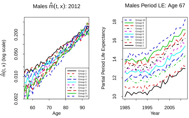
Age-specific death rates for the 10 sub-groups in 2012 are plotted in Figure 2 (left-hand plot). This plot is typical of what we see for all years 1985 to 2012. Despite the significant levels of sampling variation along each curve, we can still see a clear ranking in the plot: Group 1 has consistently the highest death rates across all ages; Group 2, the next highest; and so on down to Group 10. In particular, the rankings are what could be described as socio-economically reasonable: the more affluent someone is, the less likely they are to die in the next year compared with a less affluent person of the same age. We can also observe that relative differences in death rates between sub-groups are biggest at younger ages and smallest at very high ages.

We experimented with numerous ways of segmenting the population, but always ended up with a similar (or even narrower) spread of curves at higher ages. This finding is in line with the compensation law of mortality (Gavrilov and Gavrilova, 1991) which postulates that mortality rates for different populations tend to converge with age. This ‘law’ implies that wealth and lifestyle-related factors have a reduced impact as we age, while other, mainly genetic, factors become more significant. The narrowing gap with age is consistent with the findings of, for example, Cristia (2009) for US males, and Villegas and Haberman (2014) for males in England and Wales. In our dataset, the compensation law seems to point to convergence in the high 90s. For reasons discussed earlier, it is desirable to have distinct rankings over as wide a range of ages as possible. However, at high ages, it can be difficult to differentiate between groups. Still, we have not found any evidence that groups cross over even at very high ages in our data set, although the model does not preclude this.

It is also of interest to look at the variation in life expectancies between groups. To avoid the need to extrapolate beyond the maximum age in our dataset, we calculate

partialperiod life expectancies using a maximum age of 95, defined as the expected number of years survived from agexto agexu = 95, conditional on having survived

60 70 80 90 0.002 0.010 0.050 0.200 Group 1 Group 2 Group 3 Group 4 Group 5 Group 6 Group 7 Group 8 Group 9 Group 10

Males m^

(

)

Age m^ ( t , x ) (log scale)

1985 1995 2005

10

12

14

16

18

Males Period LE: Age 67

Year P ar tial P er iod Lif e Expectancy Group 10 Group 9 Group 8 Group 7 Group 6 Group 5 Group 4 Group 3 Group 2 Group 1

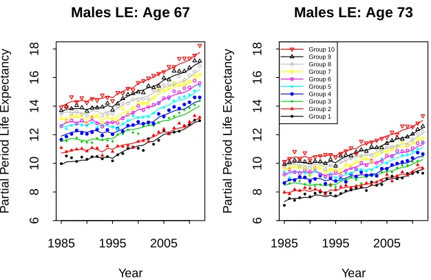
Figure 2: Left: Age-specific death rates, ˆm(i, t, x) = D(i, t, x)/E(i, t, x), between ages 55-94 for Danish males Groups 1 to 10 by age in 2012. Right: Partial period life expectancies (LE) for Danish males Groups 1 to 10 at age 67 (capped at age 95) for years 1985-2012.

measure can be approximated as follows:

LE(t, x)≈ 1 2 +

xu−1

X

y=x+1

Sp(t, x, y) +

1

2Sp(t, x, xu),

whereSp(t, x, y) = exp

−Py−1

s=xmˆ(t, s)

defines the observed period survival proba-bilities. Partial life expectancy up to age 95 is only very slightly less than complete (untruncated) life expectancy: proportionately the difference is less than 5% at all ages up to age 83 for all groups and years. (If life expectancies above age 83 are required, then it would be recommended to extrapolate the life table first before calculating full, untruncated period life expectancies.)

for sampling variation in death counts have been added. The general absence of overlap of the bands confirms that the differences between the groups and the group rankings are statistically significant.

Similar observations have been found previously with Danish data by Brønnum-Hansen and Baadsgaard (2012) using disposable income as a covariate. However, these authors only report period LE at a single age 0 and separate the population into quartiles. By contrast, we have carried out a much more detailed analysis using deciles rather than quartiles, used partial period LE over a range of ages from 55 and up, and used death rates at individual ages from 55 to 94. Our conclusion is that the use ofdisposable incomeas the key metric could be improved upon significantly. Specifically, income, on its own, does not achieve a satisfactory separation of the 10 sub-groups across all ages and all years: a problem that we have resolved through the use of the A=W + 15Y affluence index with lockdown at age 67.

The widening over time of the gap in life expectancy noted above is not unique to Denmark and can be observed elsewhere. The UK Office for National Statistics (2011) consider LEs in England and Wales by occupation group and find a widening gap between professional/managerial and unskilled manual workers; Cristia (2009) considers US males and females subdivided by lifetime earnings and also finds a widening gap over time; and Mackenbach et al. (2003) find increasing gaps in six European countries using other socio-economic measures.

3

Modelling framework and estimation

3.1

Modelling sub-group mortality

Letm(i, t, x) be the underlyingage-specific death rate for population iin year t for individuals aged x last birthday on the first of January in the year of death. A standard hypothesis in multi-population modelling is that the relationship between the death rates at given ages in two related populations should not diverge in the long run: that is, the ratio m(i, t, x)/m(j, t, x), for i6=j, should remain stable over time. This stability condition is often referred to ascoherence, and further discussion can be found, for example, in Cairns et al. (2011) and Hyndman et al. (2013).

We propose the following multi-population gravity model of the CBD-X type for underlying age-specific death rates in the 10 sub-groups:

logm(i, t, x) = β₀(i)(x) +κ₁(i)(t) +κ₂(i)(t)(x−x¯) (2)

and models the log death rate rather than the logit of the mortality rate. The non-parametric age effect was found to be necessary to preserve the mortality rankings between sub-groups over the full range of ages from 55 to 94. The κi

1(t) terms

capture changes in the level of mortality, while the κi

2(t) terms pick up changes

in the slope of the log-mortality curve relative to the baseline β₀(i)(x). As detailed below, we model period effects by incorporating a common long-term trend for all sub-groups, combined with a short-term gravity effect.

We specify the following stochastic model for the period effects:

κ₁(i)(t) = κ₁(i)(t−1)−ψκ(₁i)(t−1)−κ¯1(t−1)

+µ1+Z1i(t) (3)

κ₂(i)(t) = κ₂(i)(t−1)−ψ

κ(₂i)(t−1)−κ¯2(t−1)

+µ2+Z2i(t) (4)

where ¯κ1(t) =

1

n n X

i=1

κ(₁i)(t) and ¯κ2(t) =

1

n n X

i=1

κ(₂i)(t). (5)

¯

κ1(t) and ¯κ2(t) (Equation 5) can be interpreted as processes that govern mortality

improvements at the national level, with additional sub-group deviations from ¯κ1(t)

and ¯κ2(t) (Equations 3 and 4) that are mean reverting to prevent sub-groups from

diverging from each other. The random innovation terms Zf i(t) are multivariate

normal with mean 0 and covariances

Cov(Zf i(t), Zgj(t)) =

vf g for i=j ρvf g for i6=j

for f, g = 1,2, where −1 < ρ <1 and the Zf i(t) are independent from one year to

the next.

Theκ(₁i)(t) share a common drift,µ1, and theκ(2i)(t) share a common drift,µ2, where µ1 and µ2 need to be estimated. The components of equations (3) and (4)

−ψκ(₁i)(t−1)−¯κ1(t−1)

and −ψκ(₂i)(t−1)−κ¯2(t−1)

represent gravity effects between sub-groups (similar to Cairns et al., 2011, and Dowd et al., 2011) that prevent individual sub-group death rates from drifting away from the trend. Although 0 < ψ < 2 ensures stationarity, we restrict the range further to 0< ψ <1 to avoid oscillatory behaviour.

From Equations (3), (4) and (5), it is straightforward to show that (¯κ1(t),¯κ2(t)) is

a bivariate random walk with drift (µ1, µ2)0 and one-step-ahead covariance matrix

1 + (n−1)ρ n

v11 v12 v12 v22

.

Now define ∆1i(t) = κ

(i)

1 (t)−¯κ1(t). The ∆1i(t) are correlated AR(1) processes with

AR(1) parameter 1−ψ, that revert and add to 0, and are independent of ¯κ1(t).

We have deliberately chosen to have a single short-term contemporaneous correla-tion parameter,ρ, and a single gravity parameter,ψ, to keep the model simple (while still fitting the data well) and to reduce the computational burden. This parame-terisation implies that the one-step-ahead correlations in log death rates between all pairs of sub-groups are equal.

The gravity effect operates through the κ parameters which gravitate towards each other over time. However, the non-parametric age effects, β₀(i)(x), do not gravitate towards each other and it is the group-specific values of these parameters that keep the groups separate over the long run and in the same order as we have observed in the past. The key implication of this is that the mortality rates across different groups will not diverge systematically in the long run, but this does not imply that they will converge. The gaps between them can fluctuate without any requirement to converge to some constant value. Further, AR(1) processes (here, ∆1i(t) and ∆2i(t))

do not converge to zero. Again, the underlying principle is that of coherence, but this does not preclude periods of divergence (as some studies noted above involving educational attainment have found), it just requires that in the long run there is no divergence.

3.2

Parameter estimation

The latent state variables and process parameters were estimated using Bayesian methods, providing a rigorous and coherent framework for deriving point estimates and for assessing parameter uncertainty. This approach allows us to mitigate prob-lems that arise as a result of small population sampling variation, as recently high-lighted by Villegas et al. (2017) and Chen et al. (2017).

We seek to estimate the posterior distribution forβ (representing all of theβ(i)_(x)), κ (representing all of the κ(_ji)(t)) and φ (representing all of the process parameters

governing the dynamics of the κ(_ji)(t)), given the specific information, D, about deaths by sub-group, year and age. The posterior distribution is proportional to

f1(D|β, κ, φ)f2(β, κ|φ)f3(φ)

where: f1 is the probability of observing D(i, t, x) deaths, given β, κ and φ; f2 is

the density function for β and κ, given φ; andf3 is the prior density for the process

parameters,φ.

In practice,f1 depends only on D,β and κ, and not on φ. For modelling the

condi-tional distribution of the deaths, givenκ, we use conditionally independent normal distributions for the logD(i, t, x) (conditional onκ) with mean log ˆm(i, t, x)E(i, t, x) and variance 1/Dobs(i, t, x), where Dobs(i, t, x) is the observed number of deaths.

This choice of distribution is discussed further in Cairns et al. (2016).

formulation, β plays no role in f2: that is, our prior assumption is that the β0 (x)

are independent of each other and have an improper uniform prior distribution; and we let the deaths data drive the estimation of theβ₀(i)(x). For the given combination of equations (2), (3) and (4), we only need two identifiability constraints to uniquely identify the posterior density. We choose to fix ¯κ1(1) = 0 and ¯κ2(1) = 0. Beyond

these constraints, we also need a distributional assumption for ∆(t) ={∆ji(t) :j =

1, . . . ,10;i = 1,2} at time t = 1. We assume the stationary distribution of the underlying vector autoregressive process for ∆(1). Since 0 < ψ < 2 and the Zki(t)

are multivariate normal, the stationary distribution of ∆(t) required for ∆(1) exists and is also multivariate normal.

The use of the log-normal for deaths in combination with pre-specified variances and the chosen time series model for κ results in a log-likelihood function that is quadratic in the latent state variables, β₀(i)(x), κ₁(i)(t) and κ(₂i)(t). An advantage of this specification is that when we use Markov chain Monte Carlo (MCMC) to sample from the posterior distribution for the parameters, we can use computation-ally efficient Gibbs sampling from the conditional posterior distributions (i.e., the multivariate normal) to update theβ₀(i)(x), κ₁(i)(t) and κ(₂i)(t).

The log-likelihood does not lead to a simple conditional posterior distribution forρ, so we use the Metropolis-Hastings (MH) algorithm to updateρinstead of the Gibbs sampler (see, e.g., Gilks et al.,1996). Estimation of the posterior distribution forψ

also uses the MH algorithm for similar reasons.

The parameters v11, v22 and v12 are estimated subject to constraints. Specifically, vij = νˆvij, where the prior point estimates for the ˆvij are based on estimated

val-ues for the total Danish population, and the scalar parameter, ν > 0, has to be estimated.

Uniform prior distributions are assumed throughout, except for the following:

• A Beta(2,2) prior for ρ to ensure it remains in the range (0,1).

• A Beta(2,2) prior for ψ.

60 70 80 90

−5

−4

−3

−2

−1

Males Base Table Beta0(x)

Age

Beta0(x)

1985 1995 2005

−0.6

−0.4

−0.2

0.0

0.1

Group 1 Group 2 Group 3 Group 4 Group 5 Group 6 Group 7 Group 8 Group 9 Group 10

Kappa1(t)

Year

Kappa1(t)

1985 1995 2005

−0.005

0.005

0.015

0.025

Kappa2(t)

Year

Kappa2(t)

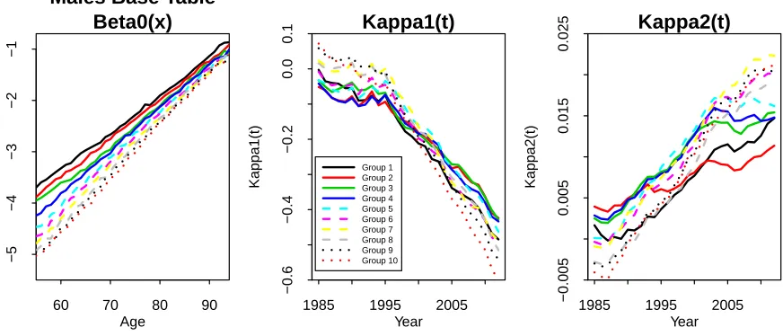
Figure 3: Estimated age and period effects for the 10 sub-populations.

4

Model fitting results and validation

4.1

Fitted age-specific death rates

Point estimates for fitted age and period effects are plotted in Figure 3. The base mortality tables (left-hand plot), represented by theβ₀(i)(x), provide the basis for the rankings of the different sub-groups in individual years. The κ(₁i)(t) period effects (middle plot) drive changes in the overall level of mortality. The individual series all follow a consistent downward trend (of generally improving mortality) that steepens after around 1995. Changes in the κ(₂i)(t) (right-hand plot) indicate how the slopes of the individual mortality curves have been changing. These have tended to rise over time (by varying amounts) indicating that mortality has improved at a faster rate at lower ages than at higher ages.

Figure 3 also reveals that the historical pattern of the time series between sub-groups exhibits a narrowing of the gap over some periods as well as some divergence over other periods – features that are quite permissible within the structure of the gravity model. Nevertheless, the model does not allow for long-term trend differentials, despite this being a major risk concern for the insurance industry. However, it would require many more years of data than currently available to us to derive a statistically significant result supporting coherence or otherwise. While exploring alternative models is, of course, important, what we present is a first step which demonstrates that the current model provides a good fit to the data.

60 70 80 90

0.002

0.010

0.050

0.500

Males Fitted m(t,x); 1985

Age

m(t,x) (log scale)

Group 1 Group 2 Group 3 Group 4 Group 5 Group 6 Group 7 Group 8 Group 9 Group 10

60 70 80 90

0.002

0.010

0.050

0.500

Males Fitted m(t,x); 2012

Age

m(t,x) (log scale)

1985 1995 2005

0.005

0.020

Males Fitted m(t,x), Age 60

Year

m(t,x) (log scale)

1985 1995 2005

0.05

0.10

0.15

Males Fitted m(t,x), Age 80

Year

m(t,x) (log scale)

60 70 80 90

0.002

0.010

0.050

0.500

Males Fitted m(t,x); 1985

Age

m(t,x) (log scale)

Group 1 Group 2 Group 3 Group 4 Group 5 Group 6 Group 7 Group 8 Group 9 Group 10

60 70 80 90

0.002

0.010

0.050

0.500

Males Fitted m(t,x); 2012

Age

m(t,x) (log scale)

1985 1995 2005

0.005

0.010

0.020

Males Fitted m(t,x), Age 60

Year

m(t,x) (log scale)

1985 1995 2005

0.05

0.10

0.15

Males Fitted m(t,x), Age 80

Year

m(t,x) (log scale)

1985 1995 2005 6 8 10 12 14 16 18 ● ● ● ● ●●● ●●●● ● ● ● ● ● ● ● ●● ● ● ●● ● ● ● ● ●● ●●● ● ●●● ● ● ● ● ● ●● ● ● ● ●● ●● ● ●● ● ● ● ● ●●●● ● ●●●● ● ●● ●●●● ● ● ● ●●● ●● ● ● ● ● ●●●● ● ● ●● ● ● ●● ● ● ●● ● ● ● ● ● ●● ● ●●

Males LE: Age 67

Year P ar tial P er iod Lif e Expectancy

1985 1995 2005

6 8 10 12 14 16 18 ● ●●● ● ●● ● ● ●●● ● ●● ●● ● ● ● ●●● ● ● ● ● ● ●● ● ● ● ●●● ● ● ●● ● ● ● ● ● ● ● ● ●● ● ● ●● ● ● ● ● ●●●● ● ● ● ● ●● ●● ●●●●● ● ● ● ● ●● ●● ● ● ● ● ●●●● ●● ● ● ● ●● ● ● ● ●● ● ● ●● ● ● ● ● ●

Males LE: Age 73

Year P ar tial P er iod Lif e Expectancy ● ● ● ● Group 10 Group 9 Group 8 Group 7 Group 6 Group 5 Group 4 Group 3 Group 2 Group 1

Figure 6: Partial period life expectancy (LE) for Danish males in Groups 1 to 10 for ages 67 (left) and 73 (right). Lines: LEs based on fitted age-specific death rates. Points: LEs based on observed age-specific death rates.

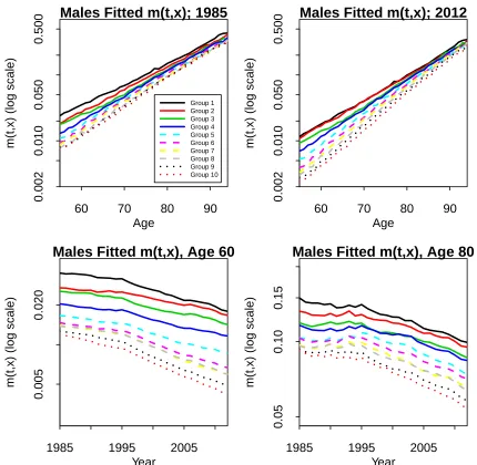
Figure 4 shows fitted age-specific death rates for the years 1985 and 2012 across all ages and for ages 60 and 80 across all years. The upper right sub-plot can be compared to the observed age-specific death rates in Figure 2 (left-hand plot). The fitted rates smooth out the noise considerably and achieve a sharp distinction between each of the sub-groups. At the same time, this clarity is achieved without losing any of the main patterns and characteristics underpinning the observed rates, such as the change in trend around 1995. From these plots of smoothed fitted age-specific death rates (and others not included here), we can confirm the findings observed earlier from plots of observed rates:

• Falling death rates over time at all ages.

• A wide gap in age-specific death rates between the least and most affluent at younger ages, and a narrower gap at higher ages.

−0.025 −0.015 0.0 0.2 0.4 0.6 0.8 1.0 Cum ulativ e Probability µ1

µ1 Posterior

0.0000 0.0004 0.0008 0.0012

0.0 0.2 0.4 0.6 0.8 1.0 µ2

µ2 Posterior

0.2 0.3 0.4 0.5 0.6 0.7

0.0 0.2 0.4 0.6 0.8 1.0 ρ

ρ Posterior

0.00 0.02 0.04 0.06 0.08

0.0 0.2 0.4 0.6 0.8 1.0 Cum ulativ e Probability ψ

ψ Posterior

3e−04 5e−04 7e−04

0.0 0.2 0.4 0.6 0.8 1.0 v11

v11 Posterior

1.0e−06 2.0e−06 0.0 0.2 0.4 0.6 0.8 1.0 v22

v22 Posterior

Figure 7: Posterior distributions for the process parameters µ1, µ2, ρ, ψ, v11 and v22.

the numerous experiments that we conducted, only affluence with lockdown at 67 produces a consistent ranking across all years and all ages.

Figure 6 plots the development of partial period LEs over time for ages 67 and 73 for each of Groups 1 to 10. The points show LEs derived from observed age-specific death rates, while the lines show LEs based on fitted age-specific death rates.

Compared with the observed LEs, the fitted LEs have more stable trends, as well as smoother gaps between the 10 groups from year to year. The model and fitting procedure achieve this without losing the essential characteristics of the observed LEs. To illustrate, the fitted LEs at both 67 and 73 (lines) track closely, but more smoothly, the level and pattern of the observed LEs (points) across all years. In particular, they pick up both the trend change in 1995 and the changing levels of inequality, such as the narrowing of the gap over time in LEs between Groups 1 and 2.

1985 to 2012. These plots highlight the wide gap between the rich and poor, even in a country with a strong health care and social security system.

4.2

Parameter uncertainty

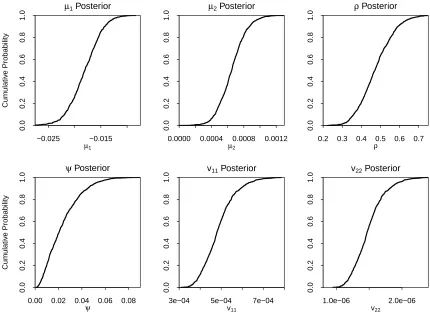
Posterior distributions for the process parameters are presented in Figure 7. Even with 28 years of data we can see that there is significant uncertainty in the drift parameters µ1 and µ2: the key parameters dictating long-term improvement rates.

As discussed below, uncertainties in µ1 and µ2 are also important determinants of

between-group correlations because of the common dependence of future death rates on the uncertain drifts. The limited number of observations also results in relatively wide posterior distributions forρ,v11andv22. The gravity parameter,ψ, can be seen

to be relatively small with, proportionately, significant variation around its median.

Although we do not plot posterior distributions for the age and historical period effects, their impact can be seen in the credibility intervals for historical death rates (i.e, up to 2012) in Figure 8. The impact of parameter uncertainty on forward correlations is discussed further in the next section.

4.3

Model validation

The stochastic model was subjected to a number of in-sample and out-of-sample model validation tests. Standardised residuals were not found to exhibit any clus-tering or obvious cohort effects and had a level of variability consistent with model assumptions, indicating a good in-sample fit and providing no evidence of overfit-ting (which would be evident if the standardised residuals had a much lower variance than 1). Estimates of age and period effects were found to be robust relative to the choice of estimation period, and out-of-sample experience was found to be consistent with projections. For further details, see Appendix D.

5

Projected mortality

5.1

Projecting future age-specific death rates

We begin by projecting future age-specific death rates. The results in this section, unless otherwise stated, include full parameter uncertainty. This means that we draw historical values for the latent state variables (the β₀(i)(x) and the κ(_ji)(t)) and the process parameters (ρ, ψ, etc.) at random from the simulated MCMC output, and then use the final year’s (2012) κ(_ji)(t) plus the selected process parameters to generate each stochastic projection scenario. (For further details, see Cairns et al., 2011, Appendix B).

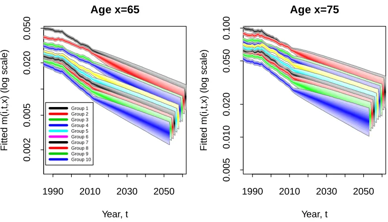
Fan charts for the underlying historical (pre-2012) and forecast (post-2012) age-specific death rates for ages 65 and 75 are plotted in Figure 8. The relative positions of the fans remain stable over the period 1985 to 2012, before widening after 2013, reflecting the projected uncertainty in future rates.

Forward correlations over varying time horizons are considered in Figure 9. These rise steadily the further into the future we project. Initially, the levels of the curves reflect the short-term contemporaneous correlations between the period effects. As the projection horizon lengthens, the shape reflects mean reversion towards the ‘national’ random walk (Equations 3 and 4).

We also see that Group 10 tends to have lower forward correlations than, e.g., Group 5, which, in turn, has lower forward correlations than Group 1. The reason is simply that Group 10 death rates are lower than Group 1 and so, in relative terms, contribute less than 10% of the risk to the national average. To illustrate, suppose

R1 andR2 are identically distributed risks, andR =pR1+ (1−p)R2. If the weight, p, attached toR1 is greater than 0.5, then R1 will contribute more to the riskiness

inR, and the correlation betweenR andR1 will be higher than that betweenRand R2.

1990 2010 2030 2050

0.002

0.005

0.020

0.050

Group 1 Group 2 Group 3 Group 4 Group 5 Group 6 Group 7 Group 8 Group 9 Group 10

Age x=65

Year, t

Fitted m(i,t,x) (log scale)

1990 2010 2030 2050

0.005

0.010

0.020

0.050

0.100

Age x=75

Year, t

Fitted m(i,t,x) (log scale)

Figure 8: Fan charts for age-specific death rates at ages 65 and 75 for Danish males Groups 1 to 10. The charts show: (a) parameter uncertainty in the fitted age-specific death rates up to 2012, and (b) combined parameter uncertainty and process risk from 2013. The lower and upper edges of the fans correspond to the 5% and 95% quantiles, respectively.

2015 2020 2025 2030 2035

0.0

0.2

0.4

0.6

0.8

1.0

●

●

●

●

●

●

●

●

Year

Correlation

●

●

●

Blue Collar Plan White Collar Plan Group 1 Group 2 Group 3 Group 4 Group 5 Group 6 Group 7 Group 8 Group 9 Group 10

Age 75

Correlations Between Group m(t,x) and Total m(t,x)

We also looked at how the ratio of death rates between different populations,

m(i, t, x)/m(j, t, x) evolved through time, scenario by scenario (Figure 8 does not allow this to be investigated), in order to check how strongly the principle of co-herence applies in simulations. Baseline ratios between different groups and ages are defined by expβ₀(i)(x)−β₀(j)(x). The long run simulated ratios are centred on these baseline values, typically with a standard deviation of about 0.14 (slightly wider than, but still consistent with, the observed historical ratios). Groups that were closer together historically have a greater chance of crossing over temporarily. For the same reason, small temporary crossovers are more likely at higher ages.

5.2

Sensitivity to the inclusion of parameter uncertainty

The level and shape of the forward correlation curve depend on whether we include uncertainty in the underlying process parameters (see, e.g., Cairns, 2013). We in-vestigate this issue in Figure 10 (left-hand plot) for Group 5 by way of illustration. This plot shows forward correlations under three experiments:

• Full Parameter Uncertainty (Full PU): full allowance for uncertainty in all pro-cess parameters and latent state variables based on the posterior distribution.

• Partial PU#1: the drift parameters µ1 and µ2 are fixed at their posterior

medians. All other elements of the posterior distribution remain random.

• Partial PU#2: the process parameters µ1, µ2, ρ, ψ and ν are fixed at their

posterior medians.

From Figure 10 (left-hand plot), we see that the curves for Partial PU #1 and #2 are almost indistinguishable indicating that uncertainty in ρ, ψ and ν has little impact on the empirical correlations. By contrast, moving from Partial PU#1 or Partial PU#2 to Full PU results in a big change. Uncertainty in µ1 and µ2 pushes

up uncertainty in ¯κ1(t) and ¯κ2(t), with a corresponding impact on uncertainty in

sub-group death rates. Since each sub-group has a common dependency on ¯κ1(t)

and ¯κ2(t) (and, hence,µ1 andµ2), correlations rise, in line with the results in Cairns

(2013).

5.3

Sensitivity to the choice of prior distribution

2015 2020 2025 2030 2035

0.0

0.2

0.4

0.6

0.8

1.0

Full PU Partial PU #1 Partial PU #2

Group 5; Age 65

Year

Correlation

2015 2020 2025 2030 2035

0.0

0.2

0.4

0.6

0.8

1.0

Rho Beta(3,3); Psi Beta(3,3) Rho Beta(2,2); Psi Beta(2,2) Rho Beta(3,3); Psi Beta(2,2)

Group 5; Age 65

Year

Correlation

Figure 10: Empirical forward correlations between Group 5 and the total popula-tion, cor (m(i, t, x),m¯(t, x)), for age 65, showing sensitivity to changes in inputs and assumptions. Left: impact of different levels of parameter uncertainty: Full parame-ter uncertainty (PU); Partial PU #1 hasµ1 and µ2 fixed at their posterior medians;

Partial PU #2 has µ1, µ2, ρ, ψ and ν fixed at their posterior medians. Other

elements of the posterior distribution remain random. Right: the three lines show sample forward correlations under three different combinations of prior distributions for ρand ψ.

estimates of the correlations are stable over a range of time horizons relative to the choice of prior.

5.4

Sensitivity to the gravity assumption

Appendix E outlines a modified model with different gravity effects forκ1 andκ2,ψ1

andψ2 respectively. Although we find that estimates for ψ1 andψ2 are significantly

6

Applications and extensions

6.1

Applications

Our analysis of mortality across a wide age range is important in the context of the intended applications. In particular, we seek to model sub-population death rates with a view to assessing how sub-groups will evolve over time relative to each other at all included ages. The resulting forward correlation term structure (as defined in Appendix A) needs to be plausible if the model is going to be useful to pension plans and insurers as a key component of their risk assessment (see, e.g., Villegas et al., 2017).

A key current example is hedging an annuity provider’s book of business using an index hedge, i.e., a hedging instrument that is based on the mortality experience of the national population. The difference between this and the mortality experience of the sub-population underlying the annuity provider’s book of business introduces basis risk in the hedge and hence reduces its effectiveness. The higher the correlation between the two populations, the lower the basis risk and the greater the hedge effectiveness (see Blake et al., 2018, section 6.3). For a real world example of an index hedge specifically designed to minimise basis risk, see the Aegon hedge designed in 2013 by Soci´et´e G´en´erale (Michaelson and Mulholland, 2015).

Another example concerns concentration and diversification of risk. Per unit of pension, a pension plan whose membership is concentrated entirely in a single af-fluence decile will potentially be exposed to greater levels of longevity risk than a similarly-sized plan whose membership is spread more evenly across all 10 deciles. The extent of this additional risk can be measured using the approach in this pa-per, and assessment of strategies to mitigate this risk will require knowledge of the forward correlation term structure. Complementing this, a plausible forward corre-lation term structure will aid assessment of the diversification benefits from having a portfolio of lives that span a range of cohorts rather than one that is concentrated in a single cohort.

6.2

Extensions

and Rosenskjold, 2017) finds consistent rankings for females across all 10 deciles.

We have not attempted to explore the many other potential covariates and pieces of information within the SD database. Our study could be extended in a number of ways. For example, we could look at the explanatory power of including other covariates, such as marital status, occupation and area of residence; how individuals migrate between different affluence sub-groups; and how to model mortality above age 95, in a way that exploits the convergence in death rates at high ages observed in Figure 4.

Although the model proposed here fits the data well, there are many variants and generalisations that could be considered. These include: alternative one-year-ahead correlation structures; alternative gravity effects (e.g., Appendix E); and more gen-eral models for the drifts of ¯κ1(t) and ¯κ2(t) (e.g., as remarked in Appendix D.3)

including allowance for trend differentials between the sub-groups.

7

Conclusions

Understanding socio-economic differences in mortality is important both to policy-makers planning state pension budgets and to private sector providers of mortality-linked products, such as pensions and annuities. We have found that socio-economic differences can be modelled more effectively through acombinationof two elements: the choice of multi-population stochastic mortality model, and the choice of predic-tive variable or covariate.

The multi-population stochastic mortality model we developed explains historical differences in the mortality of sub-groups of a national population and ensures that we obtain plausible projections of mortality improvements, which satisfy the follow-ing five criteria: (a) generate a projected trend that is consistent with the historical trend in mortality improvements, (b) produce levels of variability consistent with that observed in the historical data, (c) preserve sub-group rankings, (d) generate coherent projections across sub-groups, and (e) deliver plausible forward correla-tions between sub-groups over different ages and future horizons. We used Bayesian estimation methods to dampen the impact of sampling variation in the sub-group data – this is important for a relatively small national population such as Denmark.

the relative value of their affluence index (measured as wealth+15×income). Prior to age 67, they would be allocated to a particular sub-group annually, based on the value of the index in the previous year. In their final year before reaching age 67 – the state pension age in Denmark for much of the period under investigation – they would be allocated to a sub-group and treated as remaining in that sub-group for the remainder of their lives, a procedure we call lockdown. Lockdown at a partic-ular age combined with the affluence index was found to be critical for ensuring a consistent ranking of sub-group death rates across all years and all ages.

We experimented with a number of possible predictive variables: income, individual wealth, household wealth, and linear combinations of these. For most of the variants considered, results were not satisfactory across all ages and/or in all years. Typically, we would find consistent and unchanging mortality rankings across age for the higher (more wealthy) sub-groups, while lower sub-groups might be correctly ranked at some ages, but not at other ages. In most of our experiments, we found that (a) high income or high wealth is a strong predictor of low mortality, but (b) low income or low wealth is not a strong or consistent predictor of high mortality. For example, a 70-year-old might have little capital, but still have a good pension that allows him to live a healthy lifestyle. Another 70-year-old might have no pension, but have substantial personal savings that she can draw on to provide an adequate income in retirement – income that would not be recorded as such by Statistics Denmark.

Our approach fits Danish male data very well, preserving the socio-economic rank-ings over the historical period and without losing any of the raw data’s underlying characteristics. It also generates plausible forecasts of mortality for each of the 10 sub-group and produces a plausible correlation term structure for sub-group mor-tality rates. In the case of Danish females, there are some cross-overs in the lower socio-economic groups, but the rankings are preserved in the middle and higher groups. Our modelling framework makes no assumptions about rankings and so the model copes perfectly well if there are cross-overs – although large numbers of cross-overs would indicate that the predictive variable was fairly weak. To the best of our knowledge, no other investigators have been able to identify covariates that explain female mortality in the lower socio-economic groups better than our affluence index, although it remains a puzzle why females in Group 2 sometimes have worse mortality than those in Group 1. This is a clearly a subject for future research.

Acknowledgements

The authors wish to acknowledge the numerous discussants at conference presenta-tions of this work and especially the two referees who made many constructive and thought-provoking comments on a previous draft of the paper. MKL and CPTR gratefully acknowledge financial support from the Danish Council for Independent Research, Social Sciences, grants: 11-105548/FSE (MKL) and CREATES, Center for Research in Econometric Analysis of Time Series (DNRF78), funded by the Danish National Research Foundation. AJGC acknowledges financial support from the Actuarial Research Centre of the Institute and Faculty of Actuaries, and from Netspar under project LMVP 2012.03.

References

Blake, D., Cairns, A.J.G., Dowd K., and Kessler, A. R. (2018). Still living with mortality: The longevity risk transfer market after one decade. To appear inBritish Actuarial Journal.

B¨orger, M., Fleischer, D., and Kuksin, N. (2014) Modelling the mortality trend under modern solvency regimes. ASTIN Bulletin, 44, 1-38.

Booth, H., Maindonald, J., and Smith, L. (2002). Applying Lee-Carter under con-ditions of variable mortality decline. Population Studies, 56, 325-336.

Bound, J., Geronimus, A.T., Rodriguez, J.M., and Waidmann, T.A. (2015). Mea-suring recent apparent declines in longevity: The role of increasing educational attainment. Health Affairs, 34, 2167-2173.

Brønnum-Hansen, H., and Baadsgaard, M. (2012). Widening social inequality in life expectancy in Denmark. A register-based study on social composition and mortality trends for the Danish population. BMC Public Health, 12, 994.

Bruce, B. R. (ed.) (2015, Fall). Pension & Longevity Risk Transfer for Institutional Investors. New York, NY: Institutional Investor Journals.

Cairns, A.J.G. (2013). Robust hedging of longevity risk. Journal of Risk and In-surance, 80, 621-648.

Cairns, A.J.G., Blake, D., and Dowd, K. (2006). A two-factor model for stochastic mortality with parameter uncertainty: Theory and calibration. Journal of Risk and Insurance, 73, 687-718.

Cairns, A.J.G., Blake, D., Dowd, K., Coughlan, G.D., and Khalaf-Allah, M. (2011). Bayesian stochastic mortality modelling for two populations. ASTIN Bulletin, 41, 29-59.

Cairns, A.J.G., Blake, D., Dowd, K., and Kessler, A. (2016). Phantoms never die: Living with unreliable population data. Journal of the Royal Statistical Society, Series A, 179, 975-1005.

Cairns, A.J.G., and El Boukfaoui, G. (2017). Basis risk in index based longevity hedges: A guide for longevity hedgers. To appear in North American Actuarial Journal.

Chen, L., Cairns, A.J.G., and Kleinow, T. (2017). Small population bias and sam-pling effects in stochastic mortality modelling. European Actuarial Journal, 7, 193-230.

Chetty, R., Stepner, M., Abraham, S., Lin, S., Scuderi, B., Turner, N., Bergeron, A, and Cutler, D. (2016). The association between income and life expectancy in the United States, 2001-2014. Journal of the American Medical Association, 315 (16): 1750-1766.

Christensen, K., Davidsen, M., Juel, K., Mortensen, L., Rau, R., and Vaupel, J.W. (2010). The divergent life-expectancy trends in Denmark and Sweden – and some potential explanations. In Crimmins et al. (2010, pp. 385-407).

Coughlan, G.D., Khalaf-Allah, M., Ye, Y., Kumar, S., Cairns, A.J.G., Blake, D. and Dowd, K. (2011). Longevity hedging 101: A framework for longevity basis risk analysis and hedge effectiveness. North American Actuarial Journal, 15, 150-176.

Crimmins, E.M., Preston, S.H., and B. Cohen, B. (eds.) (2010). International Differences in Mortality at Older Ages: Dimensions and Sources. Washington, DC: The National Academies Press.

Cristia, J.P. (2009). Rising mortality and life expectancy differentials by lifetime earnings in the United States. Journal of Health Economics, 28, 984-995.

Dowd, K., Cairns, A.J.G., Blake, D., Coughlan, G.D., and Khalaf-Allah, M. (2011). A gravity model of mortality rates for two related populations. North American Actuarial Journal, 15, 334-356.

Dowd, K., Cairns, A.J.G., Blake, D., Coughlan, G.D., Epstein, D., and Khalaf-Allah, M. (2010). Backtesting stochastic mortality models: An ex-post evaluation of multi-period-ahead density forecasts. North American Actuarial Journal, 14, 281-298.

Gavrilov, L.A., and Gavrilova, N.S. (1991). The Biology of Life Span: A Quantita-tive Approach. New York, N.Y.: Harwood Academic Publisher.

Hyndman, R., Booth, H., and Yasmeen, F. (2013). Coherent mortality forecasting: The product-ratio method with functional time series models. Demography, 50, 261-283.

Juel, K. (2008). Middellevetid og dødelighed i Danmark sammenlignet med i Sverige. Hvad betyder rygning og alkohol? [Life expectancy and mortality in Denmark com-pared to Sweden. What is the effect of smoking and alcohol?]. Ugeskrift Laeger, 170(33), 2423-2427. (In Danish.)

Kallestrup-Lamb, M., and Rosenskjold, C. (2017) Insight into the female longevity puzzle: Using register data to analyse mortality and cause of death behaviour across socio-economic groups. CREATES Research Paper 2017-08, Department of Eco-nomics and Business EcoEco-nomics, Aarhus University.

Kitagawa, E.M., and Hauser, P.M. (1968). Education differentials in mortality by cause of death: United States, 1960. Demography, 5, 318-353.

Kwon, H.-S., and Jones, B. L. (2008). Applications of a multi-state risk fac-tor/mortality model in life insurance. Insurance: Mathematics and Economics, 43, 394-402.

Lee, R.D., and Carter, L.R. (1992). Modeling and forecasting U.S. mortality. Jour-nal of the American Statistical Association, 87, 659-675.

Lee, R., and Miller, T. (2001). Evaluating the performance of the Lee-Carter method for forecasting mortality. Demography, 38, 537-549.

Li, N., and Lee, R. (2005). Coherent mortality forecasts for a group of populations: An extension of the Lee-Carter method. Demography, 42, 575-594.

Mackenbach, J.P., Bos, V., Andersen, O., Cardano, M., Costa, G., Harding, S., Reid, A., Hemstr¨om, ¨O., Valkonen, T., and Kunst, A.E. (2003). Widening socio-economic inequalities in mortality in six Western European countries. International Journal of Epidemiology, 32, 830-837.

Michaelson, A. and Mulholland, J. (2015). Strategy for increasing the global capac-ity for longevcapac-ity risk transfer: Developing transactions that attract capital markets investors. In Bruce (2015, pp. 28-37).

Office for National Statistics (2011). Trends in life expectancy by the National Statistics Socio-economic Classification 1982-2006. Statistical Bulletin, 22 February.

Olshansky, S.J., Antonucci, T., Berkman, L., Binstock, R.H., Boersch-Supan, A., Cacioppo, J.T., Carnes, B.A., Carstensen, L.L., Fried, L.P., Goldman, D.P., Jack-son, J., Kohli, M., Rother, J., Zheng Y., and Rowe, J. (2012). Differences in life expectancy due to race and educational differences are widening, and many may not catch up. Health Affairs, 31(8), 1803-1813.

van Berkum, F., Antonio, K., and Vellekoop, M. (2016) The impact of multiple structural changes on mortality predictions. Scandinavian Actuarial Journal, 2016, 581-603.

Villegas, A., and Haberman, S. (2014). On the modeling and forecasting of socio-economic mortality differentials: An application to deprivation and mortality in England. North American Actuarial Journal, 18, 168-193.

Villegas, A., Haberman, S., Kaishev, V., and Millossovich, P. (2017). A comparative study of two-population models for the assessment of basis risk in longevity hedges.

ASTIN Bulletin, 47, 631-679.

Waldron, H. (2013). Mortality differentials by lifetime earnings decile: Implications for evaluations of proposed social security law changes. Social Security Bulletin, 73(1), 1-37.

Appendices

A

Forward correlations

Forward correlations can depend on a number of different random outcomes of in-terest. We mention two here, but others can be defined. For notational convenience assume that the last year of observation is year 0. Quantities of interest include death rates, m(i, t, x) and survivor indices,S(i, t, x) =Qt

s=1exp[−m(i, s, x+s−1)]

(the ex postprobability that an individual aged xat time 0 survives to time t). We define the correlation functions:

• ρm(i, t, x;j, s, y) = cor(m(i, t, x), m(j, s, y)),

• ρS(i, t, x;j, s, y) = cor(S(i, t, x), S(j, s, y)).

For both, we are likely mainly to be interested in the case t = s, and we focus our brief comments on this case.

A plausible forward correlation term structure will satisfy the following desirable criteria (building on Villegas et al., 2017):

FC1 ρm(i, t, x;j, s, y) should only be equal to 1 in the case (i, t, x) = (j, s, y)

(non-trivial correlations).

FC2 For a fixed age x, and time t, ρm(i, t, x;i, t, y) should be close to 1 for y close

FC3 For i 6= j, ρm(i, t, x;j, t, y) < ρm(i, t, x;i, t, y) (i.e., correlations between

dif-ferent ages in the same population are higher than equivalent correlations between different populations).

Having a reliable and plausible forward correlation term structure is important for a number of actuarial applications: for example, in assessing the diversification ben-efits to an insurer of holding distinctly different portfolios of lives, and in assessing the effectiveness of an index-based longevity hedge on an annuity portfolio.

A popular multi-population model that fails some of the above criteria is that of Li and Lee (2005) (see Villegas et al., 2017) in which logm(i, t, x) = A(x)K(t) +

β(i, x)κ(i, t), where A(x)K(t) is an age-period component that is common to all populations, andβ(i, x)κ(i, t) is an age-period component that is specific to popula-tioni. For two populationsiandj, for any agesxandy, whereβ(i, x) =β(j, y) = 0, we will have ρm(i, t, x;j, t, y) = 1. So the model fails criteria 1 and 2 and, almost

certainly, criterion 3.

B

Definitions of the financial variables used in the

study

Gross annual income includes all taxable income, such as wage income, self-employment income, unemployment insurance benefits, social assistance (from 1994), honoraria and all types of pension-related income. Note that non-taxable income (e.g. con-tributions to labour market pension schemes and private pension schemes) are not included in the gross annual income, as the taxes are deferred until the deccumula-tion phase.

For retired individuals, there is a break in the gross annual income variable from 1994 onwards. There are several reasons for this break. The level of old age pension benefits was increased in 1994 to compensate for the government removal of a special tax rebate previously given to retirees. Moreover, individuals living in retirement homes prior to 1994 were only given a monthly allowance, but no amount to cover rent, heating, electricity, etc., as these expenses were paid for by the government. After 1994, all individuals, irrespective of their living situation, were given the full amount of old age pension benefits or disability pension benefits.

1985 1990 1995 2000 2005 2010

10

12

14

16

18

Males LE: Age 67

Year

P

ar

tial P

er

iod Lif

e Expectancy

Group 10 Group 9 Group 8 Group 7 Group 6 Group 5 Group 4 Group 3 Group 2 Group 1

Figure 11: Partial period life expectancies for Groups 1 to 10 from 1985 to 2012 with 90% confidence bands (grey fans).

authorities. From 1987 to 1996, net wealth also included the taxable equity value of self-employed businesses (which can be negative). In 1997, a wealth tax was abolished, which resulted in the equity value of self-employed companies, the value of some mortgage deeds, shares in firms, and the value of cars, boats and mobile homes no longer being reported in the wealth measure.

C

Poisson uncertainty in empirical life

expectan-cies