Contents lists available atScienceDirect
Applied Energy
journal homepage:www.elsevier.com/locate/apenergy
A lifecycle techno-economic model of o
ff
shore wind energy for di
ff
erent
entry and exit instances
Anastasia Ioannou
a,⁎, Andrew Angus
b, Feargal Brennan
aaCranfield University, School of Water, Energy and the Environment, Renewable Energy Marine Structures–Centre for Doctoral Training (REMS-CDT) Cranfield, Bedfordshire MK43 0AL, United Kingdom
bCranfield University, School of Management Cranfield, Bedfordshire MK43 0AL, United Kingdom
H I G H L I G H T S
•
A lifecycle techno-economic model of an offshore wind farm is developed.•
Analytical consideration of OPEX linking latest reliability data to ECN O&M tool.•
Sensitivity analysis specified the most sensitive parameters on the investment NPV.•
The model was applied to different investor clusters in the wind energy market.•
Insights regarding potential minimum asking and maximum offered price are derived.A R T I C L E I N F O
Keywords: Offshore wind Techno-economic model Lifecycle
Strategic investment decision support Investor clusters
Entry and exit timing
A B S T R A C T
The offshore wind (OW) industry has reached reasonable maturity over the past decade and the European market currently consists of a diverse pool of investors. Often equity investors buy and sell stakes at different phases of the asset service life with a view to maximize their return on investment. A detailed assessment of the investment returns taking into account the technical parameters of the problem, is pertinent towards under-standing the value of new and operational wind farms. This paper develops a highfidelity lifecycle techno-economic model, bringing together the most up-to-date data and parametric equations from databases and lit-erature. Subsequently, based on a realistic case study of an OW farm in the UK, a sensitivity analysis is performed to test how input parameters influence the model output. Sensitivity analysis results highlight that the NPV is considerably sensitive to FinEX and revenue parameters, as well as to some OPEX parameters, i.e. the mean time to failure of the wind turbine components and the workboat significant wave height limit. Application of the model from the perspective of investors with different entry and exit timings derives the temporal return profiles, revealing important insights regarding the potential minimum asking and maximum offered price.
1. Introduction
With 92 wind farms in operation across European countries (in-cluding sites with partial grid-connected offshore wind (OW) turbines [1]), the OW market and supply chain have been rapidly expanding, attracting a diverse pool of investors that include Utilities, Original Equipment Manufacturers (OEMs), Independent Power Producers, Ja-panese Trading Houses, Pension Funds and Banks [2]. Broadly speaking, these investors can be segmented based on their attitude to risk (technology readiness level, track record, portfolio diversity, country, and asset phase), return expectations (Internal Rate of Return (IRR) and yield), holding length, and level of engagement[2,3].
Numerous authors have conducted research in the technical and
economic feasibility of OW farms[4–9]and related innovative concepts [10,11], and the development of cost models for OW farms[12–15]. In [4], a feasibility study was performed for the development of an OW farm installed in the Northern Adriatic Sea, in order to test the suit-ability of the region for the development of the technology, while[9] refers to a feasibility study offthe Turkish coast. Another study de-termining the profitability of an OW energy investment across different areas of Chile was performed in[8]. Kaiser and Snyder have developed models for the installation and decommissioning costs of offshore wind farms, based on existing data in European wind farms[13,16]. Myhr et al. developed a lifecycle cost model with the aim to predict the LCOE of a number of offshorefloating wind turbine concepts and compare them with their fixed monopile counterparts [5]. One of their
https://doi.org/10.1016/j.apenergy.2018.03.143
Received 9 November 2017; Received in revised form 15 March 2018; Accepted 28 March 2018
⁎Corresponding author.
E-mail address:a.ioannou@cranfield.ac.uk(A. Ioannou).
Available online 17 April 2018
0306-2619/ © 2018 The Author(s). Published by Elsevier Ltd. This is an open access article under the CC BY license (http://creativecommons.org/licenses/BY/4.0/).
conclusion was that LCOE is particularly sensitive to the distance from shore, load factor and availability. Authors in [7]develop a metho-dology for the life-cycle costing of afloating OW farm and apply it to analyse a location in the North-West of Spain and indicate the best platform option. Dicorato et al. formulated a general model to evaluate the costs in pre-investment and investment stages of OW farms and then employed this method to indicate the most suitable wind farm layout [12]. A review of offshore wind cost components was performed by [17], summarising parametric expressions and data available in lit-erature including the acquisition and installation of wind turbines and foundations, the electrical system, the predevelopment costs, etc. Shaffie et al. have also developed a parametric whole life cost model of offshore wind farms, which requires less input data in relation to other tools available[14], aiming to provide a simple framework for esti-mating the LCOE of the investment. Data were also trained in order to provide expressions for the estimation of the cost of materials used in a wind turbine, as well as the cost of the offshore substation. Finally, sensitivity analysis was performed in order to indicate the most im-pactful parameters of the model on LCOE.
Existing literature on thefinancial returns from renewable energy projects assumes that there is a single investor who owns the asset (e.g. the wind farm) throughout its entire service life[7,9,18,19]. However, recent research [3], as well as market reports [2,20,21] show that equity investors buy and sell their stakes at different phases of the OW farm life, depending on their investment strategy. To this end, a model that predicts returns over time could be useful for investors and policy makers to check the viability of the investment and to predict the temporal return profile of the investment. Additionally, the analytical consideration of the capital expenditure (CAPEX), operational ex-penditure (OPEX) and financial expenditure (FinEX) variables could contribute to the identification of input parameters that have the highest impact on the feasibility of the project.
This paper aims at addressing this challenge through developing a lifecycle techno-economic assessment framework for the prediction of lifecycle costs of OW farms, which incorporates up-to-date models for the estimation of key cost components, taking into consideration technical aspects associated with the installation and maintenance of the asset. The model developed takes into account the time that expenses occur as well as the time value of money. The high-fidelity model predicts the different costs of a typical OW farm in a lifecycle-phase-sequence pattern, by:
•
adopting the most up-to-date parametric equations found in the literature;•
developing new parametric equations where latest data are avail-able;•
including the use of industry standard ECN O&M Tool[22]for the prediction of operation and maintenance costs in conjunction with latest reliability data from[23].Compared to existing literature related to the life-cycle cost assessment of OW farms, the novelty of this paper lies on,firstly, the consideration of different equity investors with different investment strategies that buy and sell stakes at different time instances during the life of an OW farm project and the development of a relevant tool that enables such investors to as-sess the viability of their investment[3]; secondly, the prediction of the maintenance cost of the OW farm by linking the latest reliability data published in literature to the industry standard ECN O&M tool, which can account for site specific details (such as the wind profile of the location which affects the available weather window for maintenance interven-tions); and,finally the derivation of cumulative cost and revenue curves which can reflect the temporal value of the asset, providing a decision support framework to investors and, deriving insights on expected upper and lower bounds for the OW farm price setting.
Although the focus of this study is placed on Europe and especially the UK, a country with significant technical resource[24], as well as a mature market with significant secondary sales activity, the proposed
methodology can be applied to other country contexts (such as Japan, Korea and China which are regarded as significant emerging players in the OW market), provided the corresponding policy regime and cost adjust-ments (personnel cost, material costs, etc.) are taken into consideration. It, thus, needs to be highlighted that results should be treated with caution as input data have been adopted from wind farms mainly installed in North Europe, while no data currently exist for the USA or Asian offshore wind farms. Furthermore, for regions of Asia and the USA (where the frequency of hurricanes and typhoons is much higher than in Europe), existing de-sign standards should also be potentially adjusted to ensure that extreme weather phenomena are properly accounted for.
2. Methodological approach
2.1. Investor profiles in the European offshore wind market
Within the existing market, there is a variety of investors with different investment strategies and appetite for risk. OW power plants are subject to a number of uncertainties of both technical and financial nature [25], which can be encountered across the whole life of the asset by means of variability in the energy performance, capital costs, operational costs, and economics of the LCOE model[26]. As such, during the predevelopment phase, investor faces uncertainties associated with the legal, environmental survey and project management costs, among others. During the procure-ment phase, there is uncertainty in the prediction of the cost of materials of the different components of the wind farm, while during construction, variability in the cost of labour, availability and cost of installation vessels, weather conditions, along with the duration of the installation operations induce additional risk in the evaluation of the investment. Damages to the wind turbines during the operation and maintenance phase result in un-certain repair costs and loss of revenues due to downtime. Finally, varia-bility in the cost of capital can have a significant effect on the LCOE. Ac-knowledging above uncertainties within the OW energy sector [27], it becomes pertinent to identify means to systematically assess uncertainty with respect to service life valuation, hence supporting decisions of in-vestors[28]. Each investor develops their bespoke assessment and valua-tion framework projecting revenues and costs, in order to decide effectively their potential entry and exit strategies.
An analysis[3]of investor strategies, based on data from existing OW farms in the UK indicated the existence of three distinct profiles: (i) Pre-commissioning investors, (ii) Build-Operate-Transfer investors, and (iii) Late entry investors.
Late entry investors comprise third party capital investors, who are investors seeking to contribute equity capital without having an involve-ment on the core activities of the asset, such as corporate investors, in-frastructure funds and institutional investors. They undertake exclusively operational risks, entering after the commissioning of the wind farm, thus avoiding construction risks. This strategy is generally consistent with a low risk profile with stable returns. They principally purchase minority stakes in wind farm assets (mean value of 40.7%).
Pre-commissioning investors principally comprise independent energy companies, EPCI (Engineering, Procurement, Construction and Installation) contractors, and Original Equipment Manufacturers (OEMs). They can be considered as turnkey developers entering the venture at an early phase of its lifecycle to get involved in the construction and installation phase. Further, they tend to sell the majority (if not the entirety) of their stake and exit few years after the project is fully commissioned.
Finally, Build-Operate-Transfer investors comprise major utilities and independent power producers, who build and then keep the oper-ating assets in their balance sheet. Further, they tend to divest part of their stake (minority stakes) during the operating phase of the asset.
strategies with the view to identify temporal return profiles of the asset.
2.2. Overview of the developed techno-economic model for the valuation of an offshore wind energy project
In this section, the different components or programming modules of the techno-economic model of the OW energy farm are presented. The 5 main phases of an OW farm project considered are: Development and Consenting (D&C), Production and Acquisition (P&A), Installation and Commissioning (I&C), Operation and Maintenance (O&M) and Decommissioning and Disposal (D&D).
The methodological approach followed in this paper consists of the modules illustrated inFig. 1, namely: (i) the CAPEX module, which in-cludes costs during the D&C, P&A, I&C and D&D phases of the OW farm, (ii) the general site characteristics module with details on the weather conditions, site water depth, distance from port, vessels, cost of personnel etc., (iii) the FinEx module with parameters related to thefinancing ex-penditures, namely the Weighted Average Cost of Capital (WACC), infl a-tion rate, equity and debt ratio, etc., (iv) the OPEX module considering reliability data from literature, cost of personnel, materials, vessels and related maintenance processes, which will provide availability, and O&M cost estimates pertinent for the cost analysis and (v) the revenue module, which considers the net power generation, the energy policy scheme in place for supporting the technology, namely the Contracts for difference (CfD) scheme, and the market electricity price (the scheme mandates that revenues are calculated on the basis of the strike price during the first 15 years of operation of the asset and the market electricity price over the rest of its life) to derive the revenues yielded by the investment. Outputs of the model are temporal cumulative return profiles of the investment, which can support the appraisal of investment opportunities for different types of investors in various periods of a wind farm service life, taking into account the technical parameters of the problem.
3. Case study site characteristics, weather, vessel and personnel data
This section outlines the assumptions and characteristics of the re-ference wind farm, corresponding to a realistic OW farm in the UK. It also compiles data that apply to multiple phases of the lifespan of the asset,
such as the specifications of vessels and the cost of personnel. Key as-sumptions of the wind farm site are included inTable 1. The 504 MW capacity wind farm is located in the North Sea region, 36 km away from shore. Weather data (3-hourly data over a 3-year period) were retrieved from BTM ARGOSS[29]for modelling the operational phase of the asset. Weather delays during the I&C and the D&D phases were modelled by the use of an adjustment factor (ADJWEATHER), which will be described in more detail in Section4.1.3. A wind farm of approximately 500 MW ca-pacity was considered a reasonable selection, since there is a number of studies that has considered the same wind farm capacity in their baseline scenario, such as[5,14], which could facilitate comparison of results.
3.1. Vessel data
[image:3.595.44.544.58.302.2]Vessel data encompass the cost (and key characteristics) of vessels chartered for carrying out the I&C, O&M and D&D phases of the project. The specifications of the vessels (for instance, speed, day rates and mo-bilisation costs) employed for the completion of above phases are in-tegrated inTable 2, while further data regarding the number and the type of vessels used per phase and task is clarified in the respective Sections of the paper. The wind speeds are referenced at 10 m above the mean water level, while the mobilisation and demobilisation activities comprise the Fig. 1.Methodological framework.
Table 1
Case study wind farm specifications.
Wind farm characteristics Values
Wind farm Total wind farm capacity,PWT 504 MW
Projected operational life of the wind farm,n
25 years
Construction years,Tconstr 5 years
Number of turbines,nWT 140
General Site characteristics Distance to port,D 36 km Water depth,WD 26 m
Wind turbine Rotor diameter,d 107 m Hub height,h 77.5 m Pile diameter,Dpile 6 m
[image:3.595.306.554.598.745.2]cost and time allocated to the planning, preparing and modifying a vessel for a marine operation (mobilisation), and then to restoring it for release and reassignment to other operations (demobilisation).
3.2. Personnel cost
Apart from the vessel crew, additional personnel is hired to perform mechanical/electrical operations for the installation, erection and other services at a rate of £270/day[5,37]. Offshore personnel works on a shift pattern of 2 weeks“on”followed by 2 weeks“off”according to working time regulations for offshore workers[38]. Finally, a total of 12 working hours per day is assumed[5].
4. Integrated techno-economic model
4.1. CAPEX module
As previously mentioned, the CAPEX module includes costs during the D&C, P&A, I&C and D&D phases of the OW farm, which are further analysed in the following Sections.
4.1.1. Development and consenting phase (D&C)
Development and consenting costs include all costs prior to the point of financial close (i.e. the point when allfinancing agreements of the project have been signed and the conditions have been met) including project management, surveys (environmental, coastal process, Met station, sea bed, human impact), legal authorisation, front-end engineering and design and contingency costs[14,39]. Costs during D&C of the wind farm vary significantly across different sites; thus, different values of costs can be
found in literature. Indicatively, in [39] a total of £60 million for a 500 MW wind farm is reported, while in [14] costs were estimated £202.8 million for a wind farm of the same capacity. Myhr et al.[5] as-sumed a cost of £89.9 million/500 MW, while in [40] a total cost of £156.5 million/500 MW was estimated, when adjusted to the respective currency and inflation rate. In the examined case study with the total windfarm capacity of 504 MW, the cost breakdown of[14]is adopted as shown inTable 3, as a more conservative scenario.
4.1.2. Production and acquisition phase (P&A)
4.1.2.1. Wind turbines. The acquisition of a fully equipped turbine is one of the most expensive cost components of the P&A phase of the wind farm. Cost is usually expressed as a function of the turbine capacity and different parametric models have been developed to predict the cost of different sizes of turbines [11,12,15,17]. Within the context of the reference case study, the following expression has been formulated for the estimation of the wind turbine cost[14]:
= −
cT pa, 3·10 ln(6 PWT) 662,400,in£/turbine (1) where,PWTis the capacity of the wind turbine (MW). For a wind turbine of 3.6 MW, Eq.(1)results to £3.1804 million/turbine, while by adding the tower cost into the total turbine costs (which according to[39]is of the order of £1 million for a 5 MW turbine), total cost for the acquisition of the turbine and the tower accounts for approximately £3.90 million/turbine. 4.1.2.2. Foundations. A monopile configuration was assumed for the reference case study as it remains the most popular substructure up to date with a cumulative amount of 87% of all installed foundations in 2017 [1]. The cost of foundation depends largely on the type of foundation, the depth of the site, the seabed characteristics as well as, to a lesser extent, the turbine capacity, the wave and wind conditions [17]. The cost of foundation, cF pa, , was estimated by
means of a parametric expression linking the foundation cost to the turbine geometry (hub height,hand rotor diameter,d) and the water depth (WD) according to[41]:
⎜ ⎜ ⎟⎟
= + −
⎛
⎝
⎜ + ⎛
⎝ ⎛ ⎝ ⎛ ⎝
⎞
⎠−
⎞ ⎠ ⎞
⎠ ⎞
⎠ ⎟ −
c P WD
h d
320,000· ·(1 0.02·( 8))·
1 8·10 · ·
2 100,000 F pa, WT
7
2
[image:4.595.39.559.79.190.2](2) Application of the above expression to the reference case study resulted in £1.52 million/foundation. Other parametric expressions, found in the literature, link foundation cost with water depth, turbine capacity, Table 2
General data for O&M vessels and transportation equipment.
Vessel type Technician space Vessel speed (knots)
Weather limits Mob./demob. Cost (k£)
Mob./demob. Time (h)
Day rate (k£/day)
Sign. wave height (m)
Wind speed (m/s)
Crew transfer vesseli 12 26 1.8iii 16iii – – 3.25ii
Jack-up vesselsiii – 10iv 2 10 405 720/48 112.6
Heavy lift vesselvi – 9 – – 500ix – 135
Helicopterv 6 – 99 20 4.7 8/4 4.7
Diving support vessel (DSV)iii – 16 2 25 185 360v 60
Cable laying vesseliii – 14 1 10 445iii 720v 80 (Array), 100 (Export) Rock dumping vessel – 13.5vii – – 10.6viii – 13.8viii
i Source:[30]. ii Source:[31]. iii Source:[32]. iv Source:[33]. v Source:[22]. vi Source:[13]. vii Source:[34]. viiiSource:[35]. ixSource:[36].
Table 3
Cost breakdown of P&C costs.
Cost components Total cost (£ million)
Percentage over total P&C cost (%)
Legal costs,Clegal pc, 16.7 8.1%
Environmental survey costs, Csurveys pc,
19.2 9.3%
Engineering costs,Ceng pc, 1.14 0.6%
Contingency costs,Ccont pc, 126.4 61.4%
Project management cost, Cproj pc,
[image:4.595.38.286.329.429.2]as well as cost of material usage and fabrication[5,12,17]. For example, application of [17] to the baseline case study gives £1.14 million/ foundation.
4.1.2.3. Transmission system. The transmission system of the wind farm consists of: the collection system of the generated power by means of array cables, the integration of the power through an offshore substation, the transmission of the electricity from the offshore substation to shore through the export cables. Two kinds of export cables are distinguished: the offshore export cables transmit the electricity from the offshore substation to the onshore substation, and the onshore export cable which transport the power to the grid connection point.
4.1.2.3.1. Cables. Array cables organise turbines in clusters adopting various different grid schemes, such as the radial design according to which, turbines of each cluster are interconnected in a
‘string’ending at an offshore substation.
Mean Voltage (MV) submarine cables are most frequently used as array cables, while High Voltage (HV) export cables carry the stepped up voltage from the offshore substation to the grid connection point. MV cable unit costs, similarly to HV cable unit costs vary according to the cable section (i.e. data summarised inTable 4) and nominal voltage (as shown in[12]).
Export cables can be either high-voltage alternating current (HVAC) or high-voltage direct current (HVDC) depending on a number of fac-tors and especially the distance from shore. Generally, if the distance from shore is less than 50 km, AC cables would be preferred while for longer distances and in more remote wind farms, DC cables are used since HVDC cabling has no reactive power requirements resulting in lower power losses[40,43].
In general, the total cost of the cables,Ccables pa, , is calculated by the
product of the unit-length price of the cable,ci(£/m), with the number of cables,Ni, and the average length of each cable,Li(km). Protective equipment (such as J-tube seals, passive seals, bend restrictors etc.) is required to protect the cables[14].
∑
= +
=
Ccables pa ( · · )c L N C ,in £ i
i i i protection
, 1 3
(3) where,idenotes the cable type of the wind farm, namely: the MV array cables (i= 1), the HV subsea export cables (i= 2) and the HV onshore export cables (i= 3).
Retrieving data from 4C Offshore[44], a linear equation with two predictors namely, the number of wind turbines, nWT and the rotor diameterd(in m) was produced as follows:
= + − =
L1 1.125·nWT 1.055·d 122.64 (R2 0.959),in km (4) The length of the subsea export cable,L2, is assumed equal to the
dis-tance between the centre of the OW farm (where the offshore substation is located) and the shore (where an onshore substation is located), an assumption also taken in [45], which for the baseline case study is 36 km. Finally, the length of the onshore export cable,L3, is equal to the
distance from the onshore substation to the grid connection point (as-sumed to be 10 km long each). The electrical system is comprised of
33 kV array cables and two offshore substations of 336 MW HVAC transmission system. Further, the transmission assets are connected to the onshore substation by three 800 mm2132 kV subsea export cables.
The resulting costs of the electric system are summarised inTable 5. 4.1.2.3.2. Substations. The most cost efficient electric power transmission method to reduce cable losses is by means of an offshore substation, which is considered appropriate for projects located at a distance of > 20 km offshore[40]. The total offshore substation cost has been estimated by a number of authors [14,17] who derived parametric expressions linking the offshore substation cost to the total installed capacity of the wind farm. In the present study, the offshore substation cost,CoffSubst pa, , was estimated based on[12], which breaks
down the cost of offshore substation to: (1) the MV/HV transformer cost, CTR, (2) MV switchgear cost, CSG MV, , (3) HV switchgear cost,
CSG HV, , (4) HV busbar cost,cBB, (5) Diesel generator cost,CDGto supply
essential equipment when the OW farm is off, and (6) substation platform cost, CoffSubst pa, f. The expressions of the individual cost
components are the following:
=
CTR nTR·(42.688·ATR0.7513) (5)
= +
CSG MV, 40.543 0.76·Vn (6)
= +
CDG 21.242 2.069·PWF (7)
= +
CoffSubst pa, f 2534 88.7·PWF (8)
= + + + + +
CoffSubst pa, CTR CSG MV, nTR·(2·cSG HV, cBB) (CDG CoffSubst pa, f) (9) where,nTRis the number of transformers,Vnis the nominal voltage and ATRis the rated power of the transformers. Using Eq.(5)–(9)the total cost of offshore substation was calculated £60.67 million. In the context of the case study, 2 offshore substations are assumed to be placed in order to transmit the power at 132 kV. Platform 1 contains three transformers each rated 180 MVA, while Platform 3 has two 90 MVA transformers installed. Finally, the export cables connect the offshore substations with an onshore substation which further transforms power to grid voltage (e.g. 400 MW). Onshore substation cost was assumed to be half the cost of the offshore substation according to[14,39]. 4.1.2.4. Control system. More recent wind farms have integrated supervisory control (including health monitoring) and data acquisition (SCADA) systems, with the view to optimise wind turbine life and revenue generation[39]. Health monitoring of wind turbines is performed by means of sensors and control devices, gathering data that can be used for optimising operation and maintenance operations. Cost of monitoring was estimatedCSCADA pa, = 75 k£/turbine[12].
4.1.3. Installation and commission phase (I&C)
[image:5.595.307.561.80.157.2]This phase refers to all activities involving the transportation and in-stallation of the wind farm components, as well as those related to the port, commissioning of the wind farm and insurance during construction. Once a suitable number of components are in the staging area, the offshore construction starts with installation of the foundations, tran-sition piece and scour protection, followed by the erection of the tower and the wind turbines. Accordingly, the installation of the offshore Table 4
Unit costs of AC submarine cables from companies A and B. Source:[42].
Conductor size (mm2) 95 150 400 630 800 Collection system unit cost (£/m)
Company A 142 213 356 534 561 Company B 426 462 570 594 684
Transmission system (£/m)
Company A 706
[image:5.595.38.287.663.744.2]Company B 805
Table 5
Electric system cost components.
Cost component Total cost (k£) Total length of cables (km)
Array cables 28,039 147.7 Offshore export cables 84,002 108 Onshore export cables 7,778 30 Offshore substation (x2),Coff subst pa, , 121,340 –
substation, the array cables andfinally the export cables and onshore substation takes place.
4.1.3.1. Foundation and wind turbine installation. Installation costs are a function of the vessel day rates, the usage duration and the personnel costs required for carrying out the operations. Vital components of both the wind turbine and the foundation installation cost are the vessel day rates and the duration of the installation processes. The total time per trip of an installation vessel is broken down to: the travel time, the loading time, the installation time and the intra-field movement time. For the installation of monopiles a jack-up vessel can be employed with an assumed deck capacity ofVCF JU, =4 foundations. After foun-dations are secured, the transition pieces are lifted and placed on the top of the foundation pile and are then grouted. In the context of the present case study, it is assumed that the installation of monopiles and the placement of transition piece can be realised by the same vessel.
The total installation time of foundations was estimated by the following expression:
= + + + +
+
T N T n T n T T T
n T
2· · 2· · ·
·
F Instal F voy j port WT j site WT F Load porttofarm betwtrb F
WT F Lift
, , , , , ,
, (10)
where,NF voy, is the number of voyages,Tj port, is the time of jacking at
port (up/down),nWTis the number of turbines,Tj site, denotes the time of
jacking at installation site, TF Load, denotes the monopile foundation
loading time,Tporttofarmis the travel time from port to farm,Tbetwtrb F,
re-presents the time to travel between turbines, andTF Lift, is the offshore
lift/installation time of the monopile. More details on the calculation steps for the estimation of the foundation installation cost are included inAppendix A.
Turbines are installed after foundations have been placed. The vessel used both transports turbines in the installation site and performs installation. Turbines typically consist of seven components, namely nacelle, hub, 3 blades, and 2 tower sections. Onshore assembly of some of the parts of the OWT is usually performed in order to reduce lifts offshore, which can be considered risky and prone to cause delays due to wind speeds. The installation process of OW turbines is composed by the following time steps: 1. Travel/transportation time, 2. Lifting op-eration time, 3. Assembly opop-eration time (onshore and offshore), and 4. Jacking up operation time. The pre-assembly (i.e. onshore assembly) strategy followed determines the total time of turbine installation, along with the distance from the port, the number of turbines, the nameplate capacity, etc. Characteristics of different pre-assembly methods are summarised inTable 6.
For this reference case study, preassembly method 5 was used en-tailing 3 offshore lifts. Total installation time was estimated by the following expression[46]:
= + + +
T T T T T
V T Instal
T Travel j T Assemb T Lift
N JU
,
, , ,
, (11)
where,TT Travel, represents the travel/transportation time of turbines,Tj
is the jacking up operation time,TT Assemb, is the assembly operation time,
TT Lift, is the lifting operation time, andVN JU, symbolizes the number of
identical jack up vessels. Considering 12 h of total working hours, ef-fective installation time was estimated 264 days, equivalent to
1.89 days/turbine, which is in agreement with mean installation times found in literature[13]. The individual time components of the tur-bines installation time are presented inAppendix B.Finally, for the in-stallation of the tower and the Rotor Nacelle Assembly (RNA), 30 ad-ditional offshore workers are employed, and another 30 for the installation of the foundations and transition pieces. An overview of the results produced by the model on the installation costs of OW turbines and foundations is given inTable 7. A weather adjustment factor of ADJWEATHER= 0.85 was assumed in the baseline scenario to account for delays due to unpredictable unfavourable weather conditions.
4.1.3.2. Scour protection installation. The scour phenomenon takes place around structures undergoing steady current conditions, and is associated with the increase in the sediment transport capacity and erosion[47]. To ensure structural stability of the wind turbine foundation (as well as protection of cables), scour protection is usually applied. Available options to protect from scour are: placement of geotextile containers/sandbags, concrete armour units/block mattresses, grout bags/mattresses and rock armour (among others), which cover a particular area of the seabed[48]. The scour protection option employed is site-specific, i.e. at some locations the amount of protection varies with sediment and current conditions, while in others scour protection may not be needed. The input data used for the estimated mass of scour protection [49], the vessel leased for installation and the total installation time were adopted from[13,50,51]. The total effective duration for the installation of scour protection takes into account the lead time due to potential adverse weather conditions during the installation operations. As such, the total effective days were calculated by the following equation:
=
T T N
ADJWEATHER
· /24
Effectdays Scour
Scour Inst trips scour
,
, ,
(12) The total effective days correspond to the actual number of days that the rock-dumping vessel should be leased to perform the operations. As such, the installation cost of scour was estimated based on the vessel day rate and mobilisation cost (included inTable 2).Table 8presents inputs and outputs related to the calculation of the total cost and in-stallation time of the scour protection.
[image:6.595.305.558.78.188.2]4.1.3.3. Cables installation. A dedicated Cable Laying Vessel (CLV) needs to be leased for the installation of the inner array and export cables. Average installation rates of inner-array and export cables were Table 6
Pre-assembly methods characteristics.
Installation method Sub-assemblies No of onshore assemblies No of lifts/assemblies during installation(NLj)
[image:6.595.37.557.666.744.2]1 (Nacelle + hub) + 3 blades + tower in 2 pieces 1 6 2 (Nacelle + hub) + 3 blades + tower in 1 piece 2 5 3 Nacelle + (hub + 3 blades) + tower in 2 pieces 3 4 4 (Hub + nacelle + 2 blades)+ tower in 2 pieces + 1 blade 4 4 5 (Nacelle + hub + 2 blades) + 1 blade + tower in 1 piece 4 3 6 (Nacelle + hub + 3 blades + tower in 1 piece) 6 1
Table 7
Summary of results on foundations and turbines installation.
Parameter Value
Total effective days of foundations installation,TEffectdays F, 292 days
Total effective days of turbines installation,TEffectdays T, 264 days
Total effective days per foundation + transition piece 2.08
foundation effective days
Total effective days per turbine 1.89
turbine effective days
Cost of personnel employed for the installation of foundations £2.36 million Cost of personnel employed for the installation of turbines £2.14 million Total installation cost of foundations,CF ic, £102.2 million
calculated by taking into account historic data from past projects on the total length (in km) of the cables and total installation time (in days) [13]. Average installation rates were estimated approximately 1.6 and 0.6 km/day for export and inner array cables, respectively. For the installation of the subsea cables, a trenching ROV (Remotely Operated underwater Vehicle) was employed for the post–lay burial of the cables with a daily charter rate of 82.5 k£[39]. The installation cost of export and array cables was, thus, estimated based on the total duration of the installation operation, and the day rates of the CLV and the trenching ROC. As such, the installation cost of array and export cables were calculated by the following expressions:
= + +
− − −
CC array ic, TC array Inst, ·(VDR CLV array, VDR Trench, ) VMobil CLV, (13)
= + +
− − −
CC export ic, TC export Inst, ·(VDR CLV export, VDR Trench, ) VMobil CLV, (14)
[image:7.595.306.558.79.199.2]Input and output data for the cable installation are summarised in Table 9.
4.1.3.4. Substation installation. Substation is assumed to be barged on site and get installed by a Heavy-Lift vessel (HL). The installation time is comprised of the jacket foundation installation time, the grout application (if applicable) and, the installation of the substation topside. The voyage time from the port to the installation site and vice versa is estimated by:
=
T D
V 2· HL voy
S HL
,
, (15)
where,VS HL, is the speed of the heavy lift vessel used for the installation
of the substation units. The total installation time of the substation is calculated as:
= + +
TSubst Inst, (nSubst pile, ·RSubst pile, ·Dpile) Treposit TSubstjacket Inst, (16)
The symbols of Eq.(16), the input data used in the context of the case study, along with the derived results concerning the transportation and installation time of the substation foundation/topside are demonstrated inTable 10. To estimate the weight of a typical substation topside, a dataset from existing OW farms was established consisting of the substation topside weights for various wind farms whose capacities range from 60 to 630 MW (data retrieved from [52]from deployed wind farms) and a linear regression model was trained based on this dataset. As a result, the mass of the topside substation can be approximated by the following linear equation (shown inFig. 2):
= + =
WSubst top, 3.5129·PWF 388.85(R2 0.9011) (17)
The weight of the topside substation will determine the vessel that will be required with the appropriate crane capacity as shown inTable 10. Instead of assuming one topside substation of 2160 ton, two identical substations of 1080 ton were assumed. The estimation of the installation cost of the substation was based on the total effective duration of the installation operation,TSubst Inst, , and the HL vessel day
rate,VDR HLV, , and mobilisation cost,VMobil HLV, , as expressed below:
= +
COffSubst ic, TSubst Inst, ·VDR HLV, VMobil HLV, (18)
[image:7.595.38.289.86.278.2]Input and output data for the substation installation are summarised in Table 10.
4.2. OPEX module
4.2.1. Failure modes and latest reliability databases utilised
For the prediction of O&M total cost, an updated database of failure rates, number of technicians required for repairs and cost of repairs was used as input. A number of onshore wind reliability analysis exists in lit-erature, covering the whole onshore turbine as well as its subassemblies Table 8
Input and output data for scour protection installation. Sources:[16,34,50,51].
Parameter Value
Inputs
Tonnage of scour protection per unit,SPU 6,890 ton/ turbine Rock-dumping vessel capacity,VCscour 24,000 ton
Number of trips required to the installation of scour protection, Ntrips scour,
41
Total transportation time of scour protection by rock-dumping vessel,TScour Tr,
2.97 h/trip
Dumping time per trip,TScour Dump, 16 h/trip (4 h/
turbine) Loading time per trip,TScour Load, 12 h/trip
Mobilisation cost of rock-dumping vessel,Vscour Mobil, £10,650
Outputs
Total time for scour protection installation,
= + +
TScour Inst, TScour Tr, TScour Dump, TScour Load,
31 h/trip
Total effective days for scour protection installation, TEffectdays Scour,
62 days
Installation cost of scour protection,CScour ic, £872,600
Table 9
Input and output data for cables installation.
Parameter Description Value
Cables installation–inputs
Installation rate of export cable 1.6 km/day Installation rate of array cables 0.6 km/day
Cables installation–outputs
Effective days required for the installation of export cables,
− TC export Inst,
147 days
Effective days required for the installation of array cables,
− TC array Inst,
537 days
Installation cost of export cables,CC export ic− , £27.3 million
[image:7.595.306.558.235.347.2]Installation cost of array cables,CC array ic− , £87.7 million
Table 10
Input and output data for offshore substation installation.
Parameter Value
Offshore substation installation–input
Number of piles per substation foundation,nSubst pile, 4
Rate of piling the piles of the substructure,RSubst pile, 0.115 h/m
Depth of pile under the soil,Dpile 36 m
Reposition time of the vessel,Treposit 8 h
Installation time of the substation’s jacket,TSubstjacket Inst, 20 h
Offshore substation installation–output
Total effective installation days for one substation,TSubst Inst, 13 days
Total installation cost (for the 2 substations),COffSubst ic, £3.99 million
y = 3.5129x + 388.85 R² = 0.9011
0 500 1000 1500 2000 2500 3000
0 200 400 600
Weight of
offshore sub
station topside
(tn)
[image:7.595.311.553.570.719.2]Rated power output of the wind farm (MW)
[53–56]. As far as the reliability analysis of OW turbines is concerned, in [23] authors have gathered information from around 350 OW turbines with nameplate capacities ranging from 2 to 4 MW and ages between 3 and 10 years old. The failure rates used in the present analysis are pro-vided in a per turbine per year format, defined as:
∑ ∑
∑
= = =
=
λ e
E
k K
n N
e E
T
1 1
1 8760
e k T e
e , ,
(19) where,λdenotes the failure rate per turbine per year,Eis the number of intervals for which data are collected,Kis the number of subassemblies, ne k, the number of failures during the specific interval,NT e, the number of
turbines that were examined, andTe represents the total time period in hours.
∑eE= ∑kK= n
N
1 1
e k T e ,
, denotes the total number of failures in all periods per
turbine while∑eE=1 8760Te
is equal to the sum of all time periods in hours divided by the number of hours within a period of a year.
Repairs are classified as minor repairs (repairs that cost up to 1,000€), major repairs (1,000–10,000€) or major replacements (> 10,000€); a categorisation adopted by the Reliawind project which has registered failure rate data for onshore wind turbines[57]. Data on the failure rates, average repair times, number of required technicians and material costs are enclosed inTable 11.The“No cost data”category refers to repairs for whose cost data are not registered.
The mean time between failures (MTBF) is a commonly used re-liability metric for repairable items and it can be expressed as the in-verse of the failure rate, as follows:
=
MTBF λ 1
(20) As demonstrated inFig. 3, MTBF is connected to the mean time to re-pair (MTTR) and the Mean Time To Failure (MTTF) as follows[58,59]:
= +
MTBF MTTF MTTR (21)
The MTTF represents the reliability of the system while the MTTR de-notes the competence of the maintenance strategy to recover the system back to normal operation (as well as the weather window to perform maintenance operations). The latter is hence a stochastic quantity that available reliability data cannot capture and needs to be processed in
detail as will be described in Section4.2.2. Since wind turbine com-ponents undergo failures usually less than once a year (therefore MTBF > 365 days), while the MTTR usually lasts for much shorter time, above expression can be assumed equivalent toMTBF≅MTTF, which is the simplification that needs to be made in the application of the ECN O&M tool as will be described below.
4.2.2. Specification of settings for O&M costs
The detailed estimation of the O&M annual costs, downtime because of O&M activities and revenue losses caused by energy production loses was carried out through the ECN O&M tool[60], which has been used by numerous project developers and turbine manufacturers in the OW industry, and it is considered as the most comprehensive tool for O&M analysis to date[61]. It generates an average yearly estimation of the O &M cost over the lifetime of the wind farm; hence, long term average values of failure rates (as the ones outlined inTable 11) are needed as input to determine annual operating costs.
Apart from the general characteristic values of the wind farm (i.e. the number of turbines, the wind farm capacity, the power curve, etc.), met ocean data were also inserted in the software for an indicative installation site located in North Sea. Software allows for 1-hourly or 3-hourly sig-nificant wave height and mean wind speed data to be introduced; to this end, 3-hourly data was supplied by BTM ARGOSS[29].
[image:8.595.315.549.56.207.2]For framing the maintenance strategy of the reference OW farm, a Table 11
Average repair times (h), number of required technicians, material cost for different turbine components and repair category. FR: Failure rates (failures/turbine/ year), ART: Average repair times (h), RT: Required technicians, MC: Material cost (€).
Source:[23].
No cost data Minor repair Major repair Major replacement
FR ART RT FR ART RT MC FR ART RT MC FR ART RT MC
Pitch/Hyd 0.072 17 2.8 0.824 9 2.3 210 0.179 19 2.9 1900 0.001 25 4 14,000 Other Components 0.15 8 2.3 0.812 5 2 110 0.042 21 3.2 2400 0.001 36 5 10,000 Generator 0.098 13 2.4 0.485 7 2.2 160 0.321 24 2.7 3500 0.095 81 7.9 60,000 Gearbox 0.046 7 2.2 0.395 8 2.2 125 0.038 22 3.2 2500 0.154 231 17.2 230,000 Blades 0.053 28 2.6 0.456 9 2.1 170 0.01 21 3.3 1500 0.001 288 21 90,000 Grease/oil/cooling liq. 0.058 3 2 0.407 4 2 160 0.006 18 3.2 2000 0 0 0 0 Electrical components 0.059 7 2.4 0.358 5 2.2 100 0.016 14 2.9 2000 0.002 18 3.5 12,000 Contactor/circuit/breaker/relay 0.048 5 2 0.326 4 2.2 260 0.054 19 3 2300 0.002 150 8.3 13,500 Controls 0.018 17 3.2 0.355 8 2.2 200 0.054 14 3.1 2000 0.001 12 2 13,000
Safety 0.015 2 2 0.373 2 1.8 130 0.004 7 3.3 2400 0 0 0 0
Sensors 0.029 8 2.7 0.247 8 2.3 150 0.07 6 2.2 2500 0 0 0 0
[image:8.595.43.558.537.745.2]Pumps/motors 0.025 7 2.5 0.278 4 1.9 330 0.043 10 2.5 2000 0 0 0 0 Hub 0.014 8 2.4 0.182 10 2.3 160 0.038 40 4.2 1500 0.001 298 10 95,000 Heaters/coolers 0.016 5 2.7 0.19 5 2.3 465 0.007 14 3 1300 0 0 0 0 Yaw System 0.02 9 2.4 0.162 5 2.2 140 0.006 20 2.6 3000 0.001 49 5 12,500 Tower/foundation 0.004 6 2.3 0.092 5 2.6 140 0.089 2 1.4 1100 0 0 0 0 Power supply/converter 0.018 10 2.7 0.076 7 2.2 240 0.081 14 2.3 5300 0.005 57 5.9 13,000 Service items 0.016 9 2.2 0.108 7 2.2 80 0.001 0 0 1200 0 0 0 0 Transformer 0.009 19 2.8 0.052 7 2.5 95 0.003 26 3.4 2300 0.001 1 1 70,000
number of operational decisions (common within the O&M strategies of OW projects) needs to be taken. As such:
•
Four workboats (crew transfer vessels, (CTVs)) are available for O& M operations and are permanently leased on afixed contract. CTVs are used for the transportation of personnel and small components with 26knots maximum speed and maximum capacity of 15 workers.•
One helicopter is chartered to transfer technicians when response time is critical. Typically three technicians plus their equipment can be transferred by helicopter (top speed 245 km/h)[62].•
One jack-up vessel (heavy maintenance vessel) is chartered in the spot market in order to transfer and instal heavy components.•
One diving support vessel is chartered on the spot market to performunderwater inspections.
•
One cable laying vessel for replacing any damaged power cables when required.The site is close enough to shore (D=36 km) and the maintenance activities are staged out of the O&M port; thus, an accommodation vessel (or mother vessel) was not considered necessary in the baseline case study and the access time for minor repairs and inspections as well as the fair weather window were evaluated in reference to the distance from shore. General data such as maximum wave heights, wind speeds for the transportation equipment and vessel costs are shown inTable 2. Values included in the table have been retrieved and cross checked through a number of references[5,61,63–65], including a report[66]completed by the National Renewable Energy Laboratory (NREL) and the Energy Research Centre of the Netherlands (ECN) as well as from real data retrieved from 4C Offshore website[44].
The ECN O&M tool considers three types of O&M strategies, namely calendar-based, condition based and unplanned corrective. For un-planned corrective maintenance each component of the system (wind turbine and the Balance of the Plant (BOP)) is assigned an annual failure frequency. This may consist of several failure modes (fault type classes, (FTC)) with different severities and frequencies. The failure frequencies of each component of the system are introduced in the software through the MTTF. Annual failure rates from Table 15are hence transformed on a per hour basis, as follows:
=
MTTF λ 8760
,in h
(22) In the context of the baseline scenario, the components of the system considered are the ones summarised inTable 11, while the different FTCs are categorised as minor repairs, major repairs or major replace-ments (according to the Reliawind categorisation) with relative failure frequencies (RFF) calculated as:
∑
=
=
RFF λ
λ (%)
· ·100 fc
fc
fc numberofFTC
fc
1 (23)
where, fcdenotes the number of FTC. Apart from the RFF defined per FTC, the priority level as well as the repair and spare control strategy need to be defined; we set major repairs and major replacements to be of high priority and the rest to be of normal. Further data used for the definition of the unplanned corrective maintenance strategy constitute the average repair times, number of required technicians and material costs which were retrieved fromTable 11. Finally, the logistic time for major replacements for unplanned corrective maintenance was as-sumed around 250 h. Due to the multiple uncertainties as well as the lack of data for predicting condition based maintenance activities, this maintenance type was ignored.
The period for calendar based maintenance is set between 01-May to 30-September to take advantage of the expected favourable weather conditions. For calendar based maintenance, all wind turbines are
assumed to be maintained on an annual basis, through a lower cost maintenance mission, while every 5 year a larger preventive main-tenance mission is assumed to take place.
The estimation on the total number of technicians to perform the O&M operations was based on having the maximum number of manpower for 4 workboats, resulting in a total of 4 · 12 = 48 technicians. The annualfixed technician’s salary is 95 k£ for unplanned corrective maintenance, while additional crew for the calendar-based maintenance is hired with hourly wage £120/hour in the base case scenario[67].
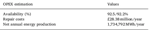
4.2.3. Operation and maintenance phase (O&M) cost estimation The costs for maintaining the OW farm were determined by both unplanned and corrective maintenance. The parameters exported through the tool were, among others, the range of availability of the wind farm, and the average annual repair cost and the power produc-tion. Results are summarised inTable 12.
4.3. Decommissioning and disposal phase (D&D)
Energy companies are obliged to remove all structures and verify the clearance of the area upon the termination of the lease. Decommissioning activities relate to the removal of the wind turbine (i.e. nacelle, tower and transition piece) as well as the balance of the plant (substation, cables and scour protection). Removal of the wind turbine and tower is done using a reversed installation method while the removal of foundation is carried out by the use of a cutting tool that removes the transition piece, while an ICM (Internal Cutting Manipulator) is used to cut the monopile at 2 m below the mud-line[68]. Cranes are used to lift the cut pieces of the turbine. Removal of mud and internal cutting can be realised by means of a workboat, while the lifting of the structure is performed by a jack up vessel. Two jack up vessels with deck space to load 5 complete WTGs with foundations are assumed. For the removal of the substation topside a heavy lift vessel is required while the jacket support structure of the substation also needs to be cut (the 4 piles) in order to get removed. As far as cables are concerned, they can be partially or wholly removed, de-pending on whether they are buried or not[69]. Cables can be cut in several sections while they are removed, hence, less expensive vessels can be employed, such as Special Operations Vessels (SOVs) or barges. In this analysis, 50% of the initial length of cables are assumed to be left in situ after the decommissioning of the wind farm (an assumption derived from discussions with wind farm operators). The scour protection may also be left in situ in order to conserve the marine life that would have grown on it. Site clearance is the final stage during decommissioning and it en-compasses the removal of the debris accumulated in a specified radius of the structure throughout the 25 years of life of the wind farm. Vessels employed for the decommissioning of the structures are assumed to have similar characteristics to the ones summarised inTable 2. Input and output values of the removal process are included inTable 13.
Further to the removal of the wind turbine components, the balance of the plant and the clearance of the area, removed items need to be trans-ported and disposed. Cost of transportation is a function of the total mass of the wind farm components,Wcomponents, the cost per ton-mile of the transportation truck,Ctruckperton mile, the capacity of truck,− Wtruck, and the distance of port from the waste facility,Dport facility, as follows− [14]:
=∑ −
C W
W ·D
transp dd
components
truck
port facility
,
[image:9.595.312.554.694.744.2](24)
Table 12
Summary of OPEX in the baseline scenario.
OPEX estimation Values
4.4. Revenue module
Levelised cost of electricity (LCOE) models consider the costs throughout the whole life of the asset. However, investors emerging in different phases of the OW farm are interested in the profitability profile of the investment from the purchasing instance until their exit point from the investment. Assessing the profitability of investing in an OW farm in different phases of its service life requires the estimation of the temporal profile of the revenues that the investment yields.
As far as the policy instruments supporting the OW industry are con-cerned, the Contract for Difference (CfD) scheme is currently in effect in the United Kingdom, which is a private law contract between a low carbon power producer and the Low Carbon Contracts Company (LCCC), a gov-ernment-owned company. According to the CfD scheme, the low carbon power producer sells the produced electricity, as usual, through a Power Purchase Agreement (PPA), to a licenced supplier or trader at an agreed reference market price. However, in order to reduce investors’exposure to variations in electricity market prices, the CfD mandates that the power producer is paid the difference between a pre-determined“strike price”
and the reference market price. If the reference price is lower than the strike price, the power generator receives the difference from LCCC; re-versely, if the reference price is higher, the power producer has to pay back the difference. The bottom line is that the power producer always gets the strike price for the electricity generated. CfDs are awarded to
power producers in allocation rounds and the amount of the strike price is determined through an allocation process, which is either based on ad-ministrative strike prices set by the Government (provided there are suf-ficient funds) or by means of a competitive auction run by the National Grid. The auctions ensure that the least expensive projects are awarded, reducing, thus, the cost passed to consumers. The scheme lasts for 15 years (while the average lifetime of an OW energy asset is 25 years), after which the electricity output is sold on the average UK electricity market price, hence imposing uncertainty to the revenues yielded by the investment after the 15th year of operation[70]. To this end, appropriate modelling of the cash inflows, along with the taxation imposed to the income needs to be conducted. For the reference case study, the baseline strike price value considered amounts to £140/MWh (which corresponds to the adminis-trative strike price for 2018/19[71]).
4.5. FinEX module
4.5.1. Depreciation and tax
Tax depreciation is available through the capital allowances regime, according to whichdrate=18%of qualifying expenditure on equipment is reduced[72]. Depreciation is a term used in accounting in order to spread the cost of the capital assets over the life span of the investment, so that the net profit in any year will reflect all the costs required to produce the output. The effect of depreciation is estimated by dividing the equipment cost of the wind farm,Cequipment, over the total life span of the asset and deducting the 18% of this annual cost from the tax pay-ment. The net tax,tnet, can then be calculated by deducting the depre-ciation credit,dcredit, from the yearly tax payment,tpayment, as shown below:
=
d C
n ·d credit
equipment
rate (25)
= −
tnet tpayment dcredit (26)
=
tpayment t Pc· gr (27)
where,tc=17%is the nominal corporate income tax rate paid every year andPgrrepresents the gross profit. Accordingly, the Net profit,Pnet, of the investment can be calculated as:
= −
Pnet Pgr tnet (28)
4.5.2. WACC and inflation
Inflation and interest rates are used to account for the time value of money. Inflation accounts for the reduction in the purchasing power of a unit of currency between two time periods, while the interest rate is the rate earned from a capital investment. Infinancial analysis, the nominal interest rate is the interest rate quoted by the banks, stock brokers etc. which includes both the cost of capital and the inflation. Real discount rate (or else real WAAC) integrates the inflation adjust-ment and the discount of cashflows according to Fisher Equation[73]:
= +
+ − ≈ −
WACC WACC
R WACC R
1
1 1
real
infl
nom infl
(29) The discount rate is determined by the source of capital as well as the estimation of thefinancial risks associated with the investment. Projects gather their capital by raising funds through debt and equity. These sources offinancing demonstrate individual risk-return profiles; hence their costs alsofluctuate. The cost of capital will correspond to the weighted average of cost of its equity and debt, with weights de-termined by the amount of eachfinancing source. The WACC is cal-culated by the following expression[74]:
= + −
WACC VE
V RoE VD
V Rd tc
· · ·(1 )
[image:10.595.40.284.76.474.2](30) where,VE is the market Value of Equity,VD is the market Value of Debt,V=VE+VD, RoE denoted the Return on Equity, and Rd the Table 13
Removal costs of wind turbine.
Parameter Value
Turbine and foundation removal–inputs
Remove time per turbine with a self-propelled jack up vessel 15 h/turbine Complete turbines (including foundations) capacity of a Jack up
vessel
5 turbines/trip
Number of jack up vessels for the removal of the wind turbines 3 Number of workboats employed for the decommissioning of the
turbines
2
Number of technicians per workboat 5 Offloading time of turbines/monopiles 8 h/item Time to cut the foundation 6 h/foundation Time to lift the item and place on the deck 11 h/item
Turbine and foundation removal–outputs
Total duration of each trip which equals the sum of the travel time to and from site, the removal time of turbines and monopile, the loading time and the intra-field movement time of the jack up vessel
244 h
Total time per trip (adjusted to weather and working hours) 26 days Total effective days for turbines and monopiles removal divided
by the number of vessels,TEffectdays TF Rem, −
243 days
Total cost of hiring technicians and workboats during the decommissioning of the wind turbines,Cvessel dd,
£4.13 million
Total cost for removing all wind turbines with monopiles,CTF dd, £83.5 million
Offshore substation removal–inputs
Pile diameters of jacket substructure 2.6 m Cutting rate of the pile 1 h/m Lifting time of topside substructure 3 h
Cut time of topside 12 h
Reposition time of vessel to each leg of the jacket substructure 8 h
Offshore substation removal–outputs
Time to cut the 4 piles 10.4 h Total time for the removal of the two substations,
− TEffectday Substat Rem,
8.7 days
Total cost for removing the two substations,CoffSubst dd, £1.18 million
Cables removal
Rate of removal of inner-array cables 600 m/day Rate of removal of export cables 875 m/day Cost of cables removal,Ccables dd, £11.9 million
Site clearance
= − + +
Area 51.5 0.41·d 0.65·nWT, in km 83.37 km2
interest rate on debt. The risk of the project significantly influences the amount of return on investment required by the investor. External ca-pital is cheaper and, thus, it is often desirable to obtain the highest possible amount of debt; however, the cost of debt depends on the specific investment risk, namely the highest the investment risk, the lower the amount that banks will be willing to lend. Average values for the components of WACC were retrieved from[75,76]for OW energy and are summarised inTable 14. Further, the real WACC is calculated by taking into account the inflation rate (inflation rate was estimated equal to 2.5% in the baseline case study, which is a realistic assumption according to UK inflation rate predictions for 2017–2018[77]).
5. Results and discussion
5.1. Cost breakdown
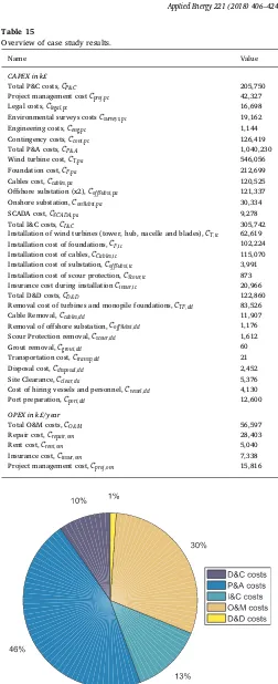
[image:11.595.305.557.34.652.2]In this Section, an overview of the case study results is presented. Table 15summarises the cost estimates of the different lifecycle phases. The total undiscounted CAPEX encompassing costs during the P&C, P& A, I&C and D&C phases amounts to £1.675 billion, while the annual OPEX was estimated £56.6 million.
InFig. 4, the relative contribution of the 5 different phases of the life cycle to the total LCOE is presented. It is indicated that the costs in-curred during the P&A phase have the largest share of the total costs (46%), followed by the O&M costs (30%). These results are consistent with a number of previous studies[14,78].
5.2. Sensitivity analysis
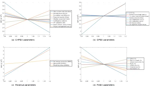
For the sensitivity analysis of the model, we have considered the wind farm general specifications, presented in Table 1 as design parameters (parameters that remain unchanged) and we have tested the sensitivity of variables found in the other modules of the model with respect to their influence on the Net Present Value (NPV) of the investment (as opposed to other works testing sensitivity of design parameters on the economic performance of the wind farm[14,79]). This should allow a targeted in-vestigation of the impact of parameters that can be influenced during the lifecycle of a wind farm of a given location.
The results of the sensitivity analysis are illustrated inFig. 5(a)–(d). The graphs include parameters which have an influence of at least ± 2% (cut-offpoint) on the NPV upon a 20% increase/decrease in their values. Under the baseline scenario, NPV of the investment was cal-culated £2.843 million at a real discount rate of 6.15% with an IRR = 10.3%. Further, LCOE was estimated £109/MWh.
Most influential CAPEX parameters appeared to be the wind turbine acquisition cost, the working hours of the personnel and the foundation acquisition cost increasing the NPV by 28% in absolute terms, upon a 20% decrease in their values, followed by the day rate of the jack up vessels and the weather adjustment factor inducing an approximately 9% change in the NPV.
As far as the OPEX parameters are concerned, the MTTF and the workboat wave height limit appeared to have the greatest influence on the NPV of the investment. In fact, a 20% drop of the wave height limit of the workboat, decreases NPV by 16%. Considering the significant
[image:11.595.304.557.84.654.2]effect of this factor on the feasibility of the project, the operator could consider measures to limit this risk; for example, through leasing workboats which could provide safe access at higher wave heights or through hiring other modes of transportation, which would allow rapid access to the WTGs regardless of weather (e.g. helicopters).
Table 14
Input data for the cost of capital calculation model. Sources:[74–76].
Values (%)
Share of equity,VE
V
30
Share of debt,VD
V
70
RoE 15.8
Rd 7
WACCnom 8.8
Table 15
Overview of case study results.
Name Value
CAPEX in k£
Total P&C costs,CP C& 205,750
Project management costCproj,pc 42,327
Legal costs,Clegal,pc 16,698
Environmental surveys costsCsurveys,pc 19,162
Engineering costs,Ceng,pc 1,144
Contingency costs,Ccont,pc 126,419
Total P&A costs,CP A& 1,040,230
Wind turbine cost,CT,pa 546,056
Foundation cost,CF,pa 212,699
Cables cost,Ccables,pa 120,525
Offshore substation (x2),CoffSubst,pa 121,337
Onshore substation,ConSubst,pa 30,334
SCADA cost,CSCADA,pa 9,278
Total I&C costs,CI C& 305,742
Installation of wind turbines (tower, hub, nacelle and blades),CT,ic 62,619
Installation cost of foundations,CF,ic 102,224
Installation cost of cables,CCables,ic 115,070
Installation cost of substation,CoffSubst,ic 3,991
Installation cost of scour protection,CScour,ic 873
Insurance cost during installationCinsur,ic 20,966
Total D&D costs,CD&D 122,860
Removal cost of turbines and monopile foundations,CTF,dd 83,526
Cable Removal,Ccables,dd 11,907
Removal of offshore substation,CoffSubst,dd 1,176
Scour Protection removal,Cscour,dd 1,612
Grout removal,Cgrout,dd 60
Transportation cost,Ctransp,dd 21
Disposal cost,Cdisposal,dd 2,452
Site Clearance,Cclear,dd 5,376
Cost of hiring vessels and personnel,Cvessel,dd 4,130
Port preparation,Cport dd, 12,600
OPEX in k£/year
Total O&M costs,CO&M 56,597
Repair cost,Crepair,om 28,403
Rent cost,Crent,om 5,040
Insurance cost,Cinsur,om 7,338
[image:11.595.72.257.666.743.2]Project management cost,Cproj,om 15,816