A Procedure for Continues Estimation of System Input Force and States
A. Kazemi Amiri1, C. Bucher2
1Department of Electronic & Electrical Engineering, Wind Energy & Control, University of
Strathclyde, Glasgow, UK
2Center for Mechanics and Structural Dynamics, TU Wien, Vienna, Austria
Keywords: Inputs/states estimation, Kalman filter, regularization
In this contribution a procedure for continuous reconstruction of system input force, along with estimation of system states is presented. For the sake of online implementation, a sliding time-window is adopted. The system input force is initially recovered from acceleration response over a finite-length time-window, using regularization technique. Afterwards, the recovered in-put force is, if necessary, fine-tuned, and the system states are estimated by application of the Kalman filtering, in order to deal with measurement uncertainty and unknown actual initial con-ditions. The successive application of regularization and Kalman filtering removes the obstacle of the unknown initial conditions of the first time- window. The initial conditions of the next time-windows are, in fact, the system states at the end of the previous time step. In order to resolve response data incompleteness, the problem is projected onto modal coordinates, while system modal parameters and mode shapes can be achieved by means of output-only techniques. The application of the proposed method demonstrates the capability of the proposed method in continuous identification of system input and states of a weather station tower.
1 Introduction
The input and state estimation problem in structural dynamics is expressed as the load (i.e. force) and response (i.e. states) estimation, where the load measurement is either difficult or sometimes impossible. In contrast, the structural response, can be measured at a much lower cost. Structural acceleration among other response types is the commonly measured response quantity in the experimental structural analysis due to the accuracy and ease of measurement. However, because of the computational and economical consideration, normally just a limited number of sensors (mostly accelerometer) can be mounted in the practice. As a consequence, there is usually an incompleteness in the response data in the sense of number and response type. The knowledge on the acting dynamic load, such as the time history itself or its power spectral density, can be considerably useful in many applications including structural reliability analysis using statistics of the input force [1] and structural health monitoring [2].
impulse response matrix, based on the assumption of the linear evolution of the force signal in order to reduce the measurement sampling rate and accordingly the size of the inverse problem [8]. They also verified their method through field experiment in cross-examination with problem simulation [9]. Bernal and Ussai investigated the stability condition of the sequential deconvo-lution, based on a sliding time-window, that can be implemented online [10]. This method has an interesting underlying, but nonetheless it is applicable if either the frequency band is limited to avoid ill-conditioning and the system initial conditions for the first time-window must be known and for preventing the error cumulation in the system states, the time-window speed has to be selected properly.
One of the first investigations, which used a Bayesian observer (Kalman filtering) was used for the inverse heat conduction problem was [11]. This technique was later implemented for input force estimation in structural dynamics (e.g. see [12]), given the displacement response data. However the displacement response cannot be readily measured in practice. Since then, the joint input-state estimation in structural dynamics experienced significant progress. For in-stance, a joint input-response estimation scheme was introduced based on minimum-variance unbiased estimation [13]. Eftekhar Azam et.al. proposed the dual Kalman filter (DKF) scheme that overperforms the AKF and minimum-variance unbiased estimation by implementing a dou-ble stage input-states estimation [14, 15]. Within another approach, Nates et.al. suggested to enhance the measured acceleration response by addition of the dummy displacement data, in-vestigating the observability issues of AKF [16]. The identifiably and stability conditions, when only acceleration response is measured, was extensively studied by [17]. These techniques es-tablished a breakthrough in the input-states estimation problem. However they cannot be either implemented online continuously over time as depending on the particular technique an a-priori information on the input force is required or displacement signal for the sake of filter stability is demanded.
The developed method in this study establishes a reconciliation between the regularization and the classical Kalman filtering techniques. Such a method can be implemented in an online manner with a time delay of order of some seconds. In order to implement this method merely the modal properties of the system are needed. The proposed method can identify the system inputs and estimates the states without a-priori knowledge on the inputs and initial conditions, only using the acceleration data.
2 Mathematical formulation and procedure algorithm
Consider the classically damped equations of motion for a multiple degrees of freedom linear system [18]:
m ¨u(t) +c ˙u(t) +ku(t) =b p(t) (1)
In the above relationu,m, c,kdenote the displacement, mass, damping and stiffness matrices
of the system, andpis the acting dynamic force. The influence input matrixbselects the loaded
degrees of freedom. The overhead dot notation represents the time derivative. The state-space
representation of Eq. 1 can be derived by introducing the state variablesx(t) =
u(t)
˙
u(t)
,
˙
x(t) =Acx(t) +Bcp(t) (2)
in which:
Ac=
0 I
−m−1k −m−1c
, Bc=
0 m−1b
The system response quantities gained by measurement are collected in the measurement vector:
d(t) =Sa¨u(t) +Sv˙u(t) +Sdu(t) (4)
Using the state variables in the measurement vector and considering Eq. 1 together with the
output influence matrices for accelerationSa, velocitySvand displacementSd, yields:
d(t) =C x(t) +D p(t) (5)
while:
C=Sd−Sam−1k Sv−Sam−1c, D=Sam−1b (6)
Solving Eq. 2 for x(t), given the initial conditionsx(t=0), renders the continuous-time solution
for the system states:
x(t) =eAc(t−t0)x(0) +
Z t 0
eAc(t−τ)B
cp(τ)dτ (7)
The first and second parts of the solution pertain to the transient response, caused by the initial conditions, and steady state response to the dynamic loading, respectively. The recursive form for the above solution is obtained by discretization in time. This solution together with the discretized measurement vector renders the discrete-time model of the system,
xk+1(t) =A xk(t) +B pk(t) (8a)
dk+1=C xk+D pk(t) +εεε (8b)
where:
A=eAc(∆t), B= [A−I]A
c−1Bc (9)
The above model can take into account the measurement noise εεε in terms of Gaussian white
noise process with the covariance matrix Rεεε =E[εεε εεεT]. If the system input force is known,
then Kalman filtering can minimize the mean square error in the estimated system states in the presence of measurement noise [19].
The input-output relationship can be established based on the Eqs. 8a and 8b.
d[0,n]=r0x0+h p[0,n] (10)
The matrixhis referred to as the impulse response matrix (IRM). The system input can possibly
be recovered from the steady state response, provided the initial conditions response is known and subtracted from the measured response data. This is a restricting condition in practice, though. Classically, the mathematical problem of solving Eq. 10 for the input is sorted among the ill-posed problems. There exists plenty of different techniques for this purpose. In our proposed procedure, any regularization scheme might be used for the sake of continuous input reconstruction. However for application in this study, it is essential that the regularization extent can be automatically and actively determined, too. A well-known, and perhaps the most famous approach in this context is the so-called Tikhonov regularization,
argmin
p[0,n]
n
b[0,n]−h p[0,n] 2 2+λ
2 p[0,n]
2 2 o
where the steady state response equals b=d˜[0,n]−r0x0 and λ stands for the regularization
parameter.
If the system response is measured only at a limited number of degrees of freedom and the number of unknown input forces exceeds that of the measurements, then system order reduction techniques (See e.g. [20]) or modal truncation can be applied to make the system of linear equations in Eq. 10 determined. In this contribution the equations of motion are projected onto the modal coordinates. As such the system’s modal input and states will be estimated. This idea is also useful, if it is to study the destructive vibration modes. Note that, the modal parameters and mode shapes are also required to generate the IRM and modal responses. Therefore, an operational modal analysis (OMA) technique can be employed for this purpose. The readers are referred to the author’s works for more information [8, 9].
The system input and states are continuously reconstructed according to a moving time-window with a predefined length. A key point of the continuous input-output reconstruction is the automatic determination of the optimal regularization parameter, corresponding to each time-window. This is essential to resolve the effect of unknown initial condition. One of the tech-niques for determination of the optimal regularization parameter is using the L-curve. In each time-window, the regularized solution of the input is inserted into a double Kalman filtering scheme for fine-tuning of input force and system states estimation. Our preliminary simulation results identifies two sources of error in the inverse input solution. Firstly there exist noise magnification in the higher frequencies which can be suppressed by fine tuning of input force.
The initially identified input is fine-tuned by assuming the input as a zeroth order random walk
stochastic process. Another discrepancy is observed in terms of low frequency deviations due to use of acceleration data. However normally the measured response signal is high-pass filtered over the low-frequency range, which resolves such a problem.
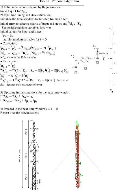
The proposed algorithm for the automated and continuous input/state estimation is briefly pre-sented in Table 1.
3 Results
The performance of the proposed method is evaluated for reconstruction of the fluctuating part of the modal wind load and system states of a mast structure. The case study is a guyed mast, serving as a weather station tower. The structural details of the mast side view and the sketch of its finite element model (FEM) is represented in Fig. 1. The mast structure consists of three parts, each of which is made of three main legs with the horizontal and diagonal braces. The guys connected to the third part of the mast, also provide lateral support for the structure from three sides. The full-scale finite element model of the structure, consisting of Euler-Bernoulli beams, is established in slangTNG. The structural damping is set up according to Rayleigh damping, such that the damping ratio of the first two modes are identically set to 1%. The first three eigenfrequencies of the structure together with the damping ratios are given in Table 2..
The wind loads are derived from the linear fluctuating wind pressure, and applied in two in-plane perpendicular directions along the mast, given a wind speed power spectral density (PSD) function. The fluctuating wind speed along the mast is simulated as an 18-variate single dimen-sional stationary random process, independently in each direction. The resultant fluctuating wind pressure components associated with the wind speeds, acts on the projected exposed areas of the mast elements, which renders the exerted wind load. The reference mean wind speed
at the height of 10m was taken equal to 10 m s−1, and the frequency band of the wind speed
Table 1: Proposed algorithm
1) Initial input reconstruction by Regularization: Solve Eq. 11 for ˜p[0,n]
2) Input fine tuning and state estimation:
Initialize the time-window double-step Kalman filter:
Initial error covariance matrix of input and states andlpS−0,lxS−0: Set positive random variables forl=0
Initial values for input and states: lp
0=p˜0 lx
0: Set random variables forl=0
•Correction: l
p+k+1=lp+k+1−lpK+k+1(lpdk+1−lpC l
p−k+1) l
x+k+1=lx+k+1−lxK+k+1(lxdk+1−lxC l
x−k+1)
K+k+1denotes the Kalman gain
•Prediction: l
p−k+1=lp+k
lp
S−k+1=lpS+k +lRp, lRp=E[θθθpθθθTp] =E[˜p[0,n]p˜T[0,n]] l
x−k+1=Alx+k +Blp+k
lx
S−k+1=AlxSk+AT+lRεεε,
lR
εεε =E[εεε εεε
T]: here assumed zero
Sk+1denotes the covariance of error
3) Updating initial conditions for the next time-window l+1xS
0=lxSn,l+1x0=lxn l+1pS
0=l+1pSn,l+1p0=lpn
4) Proceed to the next time-windowl=l+1: Repeat over the previous steps
{
!
p[0,n] → ! k= 0 n → l l+1 !
l+1x S0=
lx Sn
l+1x0=lxn ! → ! k= 0 n 1 2 3
4 l+2
t
!
!
l−1
[image:5.612.93.496.68.385.2]3 0 f t = 9 .1 4 4 m Pa n e l Pa rt 1 Pa rt 2 Pa rt 3 S1 S2 S4 S3 S5 S6 S7 x y z
Table 2: Natural frequencies and damping ratios derived from mast finite element model
Mode 1 2 3
Eigenfrequency (Hz) 3.031 3.227 3.337
Damping ratio (%) 1.00 1.00 1.00
configuration along the mast at seven locations, as marked by[S1 :S7]in Fig 1. The response in
two horizontal directions was measured at[S1,S3,S5,S7], while at the rest of the locations the
response was additionally obtained just in one direction. The main interest is to implement the proposed method for input reconstruction in the frequency range of the first three modes, that are more relevant to wind excitation. The operational modal analysis is performed by frequency domain decomposition (FFD) method [21].
The OMA results shows that the first mode was weakly excited, while the second mode can be properly identified. Thus for the sake of comparison, the presented algorithm is evaluate for the first and second modes. The natural frequencies of the first and second modes are identified to
be 3.026 and 3.227Hz. The damping ratio of the first and second modes are equal to 1.05% and
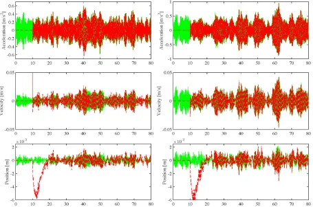
0.96%, respectively. The sampling rate was taken equal to 300 samples per second. The length of time-window is set to 10 seconds, in order to increase the stability of the reconstructed input force in lower part of the frequency band. Figs. 2 and 3 illustrate the estimated input modal wind forces and system states from the acceleration response with 3% noise level. For the first mode, there are two points that should be pointed out. Firstly, there is a constant drift between the power spectrums of the reconstructed and actual values. This arises from the fact that this mode is weakly excited, and thus its corresponding decomposed modal acceleration has higher power that the actual oner, over the frequency range. Secondly, this mode seems to be highly
coupled with another mode around 11Hz. Since such a mode was not taken into account in
the modal decomposition, its contribution appears as a fictitious peak in the reconstructed input force. These two issues are the source of the inaccuracy in the time series of the reconstructed input wind force in the first mode. However, these shortcomings are associated with the system identification. On the other hand, the input wind force of the second mode only suffers the
contribution of the coupled mode at 14 Hz, which seems to be negligible according to the
input force signal in the time domain. In both modes, the very low frequency components (ca.
60.35Hz) can not be reconstructed well. Nevertheless, one can increase the time-window
length at the expense of higher computational cost, but the question is how important could be the signal resolution in the very low frequencies for a specific purpose.
4 Conclusion
Time [s]
0 10 20 30 40 50 60 70 80
Force [N]
-2 -1 0 1
Time [s]
0 10 20 30 40 50 60 70 80
Force [N]
-2 -1 0 1
Frequency [1/s]
10-1 100 101 102
Force PSD [s(N
2)]
10-10 10-5 100
Frequency [1/s]
10-1 100 101 102
Force PSD [s(N
2)]
[image:7.612.80.516.66.271.2]10-10 10-5 100
Figure 2: Comparison of reconstructed and actual wind load inputs of mast structure. Input force time histories (top), input force PSD (bottom). Left: first mode, right: second mode.
Actual input (solid green), fine-tuned reconstructed input (dashed red)
Figure 3: Comparison of estimated and actual system states of mast structure under wind load. Left: first mode, right: second mode. Actual state (solid green), states by fine-tuned input
[image:7.612.76.531.378.679.2]5 Acknowledgment
The authors would like to acknowledge “Austrian Science Funds (FWF)” for the financial sup-port of the “Vienna Doctoral Programme on Water Resource Systems (DK-plus W1219-N22), TU Vienna” and “Wind Energy & Control centre, University of Strathclyde”. The technical supports of the DK colleagues for the regular access to the weather station mast of the “Hy-drological Open Air Laboratory Petzenkirchen” (HOAL), Lower Austria, is highly appreciated, too. The authors would also like to thank Professor R¨udiger H¨offer, director of the “Center for Wind engineering and Fluid Mechanics” at Bochum Ruhr University, Germany, for the comple-mentary research supports.
REFERENCES
[1] C. Gasser, C. Bucher, An optimized strategy for using asymptotic sampling for reliability analysis, Structural safety 71 (2018) 33–40.
[2] C. Papadimitriou, C. Fritzen, P. Kraemer, E. Ntotsios, Fatigue predictions in entire body of metallic structures from a limited number of vibration sensors using kalman filtering, Structural control and health monitoring 18 (2011) 554–573.
[3] A. N. Tikhonov, V. Y. Arsenin, Solution of ill-posed problems, Wiley, New York, 1997.
[4] P. C. Hansen, Regularization, gsvd and truncated gsvd, BIT 27 (1987) 543–553.
[5] L. Wang, Y. Xie, A new conjugate gradient method for the solution of linear ill-posed problem, Applied and computational mechanics (2012) 1–3.
[6] L. Nordstroem, A dynamic programming algorithm for input estimation of linear time-variant systems, Computer methods in applied mechanics and engineering 195 (2006) 6407–6427.
[7] B. Qiao, X. Zhang, J. Gao, R. Liu, X. Chen, Sparse deconvolution for the large-scale ill-posed inverse problem of impact force reconstruction, Mechanical Systems and Signal Processing 83 (2017) 93–115.
[8] A. Kazemi Amiri, C. Bucher, Derivation of a new parametric impulse response matrix utilized for nodal wind load identification by response measuremen, Journal of Sound and Vibration (344) (2015) 101–113.
[9] A. Kazemi Amiri, C. Bucher, A procedure for in situ wind load reconstruction from struc-tural response only based on field testing data, Journal of wind engineering and industrial aerodynamics.
[10] D. Bernal, A. Ussia, Sequential deconvolution input reconstruction, Mechanical Systems and Signal Processing (50-51) (2015) 41–55.
[11] P. Tuan, C. Ji, L. Fong, W. Huang, An input estimation approach to on-line two-dimensional inverse heat conduction problem, Numerical heat transfer B (293-363).
[13] S. Gillijns, B. D. Moor, Unbiased minimum-variance input and state estimation for linear discrete-time systems, Automatica 43 (2007) 111–116.
[14] S. E. Azam, E. Chatzi, C. Papadimitriou, A dual Kalman filter approach for state esti-mation via output-only measurements, Mechanical systems and signal processing (60-61) (2015) 866–886.
[15] S. E. Azam, E. Chatzi, C. Papadimitriou, Experimental validation of the Kalman-type filters for online and real-time state and input estimation, Journal of vibration and control.
[16] F. Naets, J. Cuadrado, W. Desmet, Stable force identification in structural dynamics using kalman filtering and dummy-measurements, Mechanical systems and signal processing 50-51 (2015) 235–248.
[17] K. Maes, E. Lourence, K. V. Nimmen, E. Reynders, Design of sensor networks for instan-taneous inversion of modally reduced order models in structural dynmaics, Mechanical Systems and Signal Processing 52-53 (2015) 628–644.
[18] F. Ziegler, Mechanics of solids and fluids, 2nd Edition, Springer, New York, 1998.
[19] K. J. Astr¨om, R. M. Murray, FeedbackSystems, An Introduction for Scientists and Engi-neers, Princeton University Press, 2008.
[20] A. Kazemi Amiri, C. Bucher, Identification of fluctuating wind load distribution along the structure’s height inversely by means of structural response, Proceeding of Advances in Wind and Structures (AWAS14), Busan, South Korea, 2014.
[21] R. Brincker, L. Zhang, P. Andersen, Modal identification from ambient responses using frequency domain decomposition, Proceeding of the international modal analysis confer-ence (IMAC), Texas, USA, 2000.