Sampling CAD models via an extended teaching–learning-based optimization technique

Sampling CAD Models via an Extended Teaching-Learning-Based Optimization

Technique

Shahroz Khan∗,1 _{Erkan Gunpinar}1 1_{Istanbul Technical University}

Abstract

The Teaching-Learning-Based Optimization (TLBO) algorithm of Rao et al. has been presented in recent years, which is a population-based algorithm and operates on the principle of teaching and learning. This algorithm is based on the influence of a teacher on the quality of learners in a population. In this study, TLBO is extended for constrained and unconstrained CAD model sampling which is called Sampling-TLBO (S-TLBO). Sampling CAD models in the design space can be useful for both designers and customers during the design stage. A good sampling technique should generate CAD models uniformly distributed in the entire design space so that designers or customers can well understand possible design options. To sampleNdesigns in a predefined design space,N sub-populations are first generated each of which consists of separate learners. Teaching and learning phases are applied for each sub-population one by one which are based on a cost (fitness) function. Iterations are performed until change in the cost values becomes negligibly small. Teachers of each sub-population are regarded as sampled designs after the application of S-TLBO. For unconstrained design sampling, the cost function favors the generation of space-filling and Latin Hypercube designs. Space-filling is achieved using the Audze and Eglais’ technique. For constrained design sampling, a static constraint handling mechanism is utilized to penalize designs that do not satisfy the predefined design constraints. Four CAD models, a yacht hull, a wheel rim and two different wine glasses, are employed to validate the performance of the S-TLBO approach. Sampling is first done for unconstrained design spaces, whereby the models obtained are shown to users in order to learn their preferences which are represented in the form of geometric constraints. Samples in constrained design spaces are then generated. According to the experiments in this study, S-TLBO outperforms state-of-the-art techniques particularly when a high number of samples are generated.

Keywords: Teaching-Learning-Based Optimization, Design Sampling, Computer-Aided Design, Generative Design

1. Introduction

Engineering and industrial product design is a goal-oriented, constraint-based decision making process. The product obtained after this process should satisfy the consumers’ needs, not just in its functional performance, but also its external appearance. The design process becomes more complex and time consuming if the products appearance is valuable to the consumers. At the initial stage of the design process, there may be no or few CAD models available for prototyping or design validation analysis. Design engineers form the design space for the CAD model using design specifications. The CAD model is modified to obtain geometric variations, some of which are inspected visually and validated based on the computer simulations or customer preferences. We think that a CAD model sampling technique can be beneficial for the designers during the design and validation stages. Moreover, CAD models sampled uniformly throughout the design space can form a better response surface, which can alleviate the computational burden of the computer-aided analysis (CAE) at the design validation stage[1].

The design space of a CAD model is defined by a set of design parameters, each with lower and upper bounds. Each design parameter represents a dimension in the design space. CAD model sampling is a high-dimensional

∗

Email:[email protected], [email protected]:Istanbul Technical University, School of Mechanical Engineering, Inonu

Nomenclature

n Number of subjects/parameters

N Number of designs to be sampled in the design space

Xk kthlearner

Mj Mean result of the learner in the jthsubject (dimension)

Xbest Teacher (learner with the best fitness when considering all the subjects)

TF Teaching factor

xl_m,j Lower bound for the jthdesign parameter for the designm xu

m,j Upper bound for thej

th_{design parameter for the designm}

P Population

pg gthsub-population ofP

s Size of each sub-population

T Vector consists of teachers of sub-population

xp,j,xq,j Scaled parameter values for the jthsubject of the teacherspandqinT

U(T) Cost function

U1(T) Potential energy (term for obtaining space-filling design)

U2(T) Term for obtaining non-collapsing designs

U3(T) Term for constraint handling mechanism

α User-define parameter adjusting weight for theU2(T) term

λpq Number of coordinates that two designs,pandqshare

β Weight for theU3(T) term

φt tthgeometric constraint

nc Number of geometric constraints

constrained optimization problem as there are generally a high number of design parameters and design constraints (i.e., relations between the parameters).

In this work, the space-filling criterion [2, 3, 4, 5, 6, 7, 8, 9, 10, 11, 12, 4, 13, 14, 15] is considered during sampling; this criterion favors the generation of CAD models spreading throughout the design space. Such sampling can give a better understanding of the design options in the design space for the designers. However, it tends to place a large portion of the designs at the corners and on the boundaries of the design space [5], especially in the case of high-dimensional sampling problems. To overcome this issue, designs are searched as far as possible in the class of Latin hypercube (LH) designs [16, 17, 4, 18, 6, 7, 8, 19, 11, 20, 21]. Therefore, thenon-collapsingness

criterion is also considered, so that the sampled designs do not share any design parameter values. Furthermore, non-collapsing designs are preferable in sampling CAD models, which are further tested in the validation step via computer simulations (i.e., CAE). The designs of experiments are crucial in CAE, which has the major goal of determining which design parameters have the greatest effects on the simulation results. Most CAE analyses are computationally expensive, and running the analysis for collapsing designs would ultimately result in unnecessary computational costs [4, 18]. As a result, this work takes the space-filling and non-collapsing properties into account while sampling CAD models. The degree of non-collapsingness is controlled with a weight term, which gives the designer the ability to create either completely non-collapsing or semi-non-collapsing designs.

S-TLBO technique.

Four major contributions are made into the standard TLBO approach in order to extend its ability for design sampling which are listed below:

(1) The population is divided intoNnumber of sub-populations. Teachers of sub-populations will be regarded as the sampled designs, which are obtained by the S-TLBO approach.

(2) A cost (fitness) function is integrated into the TLBO technique in order to sample designs that spread evenly in the design space.

(3) A penalization technique is introduced in the TLBO to obtain designs having non-collapsing (NC) property as much as possible.

(4) A static constraint handling mechanism [30] is utilized in the S-TLBO technique to sample designs in the con-strained design space so that sampled designs satisfy the predefined design constraints.

Figure 1: Illustration of the outcomes of proposed S-TLBO

The remainder of this paper is organized as follows: Section 1.1 reviews relevant literature. Formulation of original TLBO algorithm is described in Section 2. Section 3 discusses the proposed approach for generating new designs. Section 4 illustrates test models that are used for the experiments. The numerical results of the proposed approach are given in Section 5. Concluding remarks and opportunities for future work are presented in Section 6.

1.1. Related works

Our approach mainly depends on Teaching-Learning-Based Optimization (TLBO) and on the sampling of space-filling designs. Below, we discuss some previous works done by different researchers in these fields.

TLBO:TLBO was proposed by Rao et al. [22] and several improvements have been made on the technique in order to improve its performance and to expend its application in different fields. Rao and Patel [31] introduced the concept of elitism in the original TLBO to solve a series of constrained optimization problems. Another variation of TLBO calledOD-based TLBOwas introduced by Satapathy et al. [32]. OD-based TLBO combines the concept of traditional TLBO and orthogonal designs to improve its convergence performance. Chen et al. [33] enhanced the search ability of TLBO by introducing the concept of local learning and self-learning. A perturbation based scheme was introduced by Ouyang et al. [34] in order to prevent TLBO from getting trapped in the local optima. Patel and Savsani [35] and Yu et al. [36] incorporated the concept of Pareto dominance into TLBO to solve multi-objective constrained-based optimization problems.

TLBO and its variations have also been implemented to different fields such as science and engineering, includ-ing manufacturinclud-ing and mechanical engineerinclud-ing, data clusterinclud-ing [37] and feature selection [38] and combinatorial optimization [39, 40, 41]. In manufacturing and mechanical engineering, TLBO has been used for cloud manu-facturing [42], advanced finishing processes [43], heat exchangers [44], parameter optimization of selected casting processes [45], optimization of aerodynamic shapes [46] and mechanical design optimization [22].

Another algorithm for space-filling designs was proposed by Cioppa and Lucas [11]. However, their algorithm is computationally expensive because it requires long run times. Asliced space-fillingdesign technique was introduced by Qian and Wu [9], where the design space is further sub-divided into small design spaces and sampling is then performed in the sub-spaces. Prescott [20] performed complete and partial enumeration searches to investigate the space-filling properties of orthogonal-column Latin Hypercube. Lekivetz and Jones [3] introduced an algorithm for contracting non-collapsing space-filling designs for higher dimension unconstrained input regions. Grosso et al. [18] proposed heuristic algorithms based on the Iterated Local Search (ILS) to create the maximin LH designs. Khan et al. [48] developed a spatial simulated annealing based sampling technique, and Khan and Gunpinar [49] proposed an Extended Latin Hypercube Sampling (ELHS) technique for automatic sampling and generation of CAD models. In ELHS to sample designs in the class of Latin Hypercube enumeration is preformed in each stratum of hypercube and variety of designs are selected based on a similarity constraint. ELHS has the ability to perform sampling in constrained and unconstrained spaces but it does not have good space-filling property.

There is a considerable amount of research that has been done on optimal selection of space-filling designs. However, most works done by researchers are proposed for the unconstrained design spaces. The research problem becomes more complicated when a selection of designs has to be performed in a constrained and high-dimensional design space like in the research of this paper. Myˇs´akov´a and Lepˇs [50] proposed a technique to perform sampling for constrained spaces. This technique is based on the triangulation of admissible space by Delaunay Triangula-tion method. Although this technique has good space-filling property, it is just applicable to only two dimensional constraint problems. A constrained Latin Hypercube technique to solve constrained problems was demonstrated by Petelet et al. [19] and Benkov´a et al. [14]. Dragulji´c et al. [17] proposed a CoNcaD algorithm for constructing non-collapsing and space-filling designs for bounded nonrectangular design spaces. Trosset [15] and Stinstra et al. [13] used maximin criterion for the construction of space-filling designs in the constrained 10-dimensional design space. The technique proposed by Stinstra et al. [13] does not guarantee the sampled designs to be non-collapsing. Fuerle and Sienz [4] proposed a method to produce Latin Hypercube designs in constrained spaces. This method has some drawbacks such that it cannot be implemented for high-dimensional sampling problems more than 3D. Furthermore, it does not produce good results for a design space where infeasible designs are spread irregularly. S-TLBO, proposed in this paper, has the ability to obtain space-filling designs in more than 3Ddesign spaces. S-TLBO also ensures sampling space-filling designs in the constrained design spaces where distribution of infeasible designs is highly irregular.

2. Teaching-Learning-Based Optimization (TLBO)

TLBO starts the optimization process by randomly generating a population of initial solutions for a given size within the defined design space. The solution is improved by undergoing two phases: teacher phase and learner phase. A population denoted byPis considered as a class of learners. Design variables are analogous to the subjects offered to learners in the class. In the teacher phase, the best solution in the entire class is selected as a teacher and this teacher tries to improve the quality of learners by sharing his/her knowledge with them. The quality of the teacher has significant influence on the quality of learners. In the learner phase, learners try to improve their quality by interacting with other learners. The detailed description of TLBO can be found in [22, 51]. The teacher and learner phases of TLBO are summarized in the subsequent sections.

2.1. Teacher phase

In the teacher phase, the teacher is selected based on the fitness value of cost function and attempts to increase the mean result of the entire class. Suppose there arennumber of subjects (i.e. design parameters) offered tosnumber of learners. Thekthlearner is denoted byXk=[xk,1,xk,2,xk,3, . . . ,xk,n]. At any sequential teaching or learning iteration,

i,Mj,iis the mean result of the learners in a particular subject j(j=1,2, . . . ,n). The learner with the best fitness when

considering all the subjects is chosen as a teacher (denoted byXbest,i) for that iteration. The position of each learner in

theith_{iteration is updated using Equation (1).}

x0_k,j,iis the updated value ofxk,j,i, andxbest,j,iis the result of the best learner (i.e., teacher) in the subject j. riis a

random number in the range [0−1]. TF denotes the teaching factor whose value can be either 1 or 2 and computed

using the following formula:TF =round[1+rand(0,1){2−1}]. X0k,iis accepted if it gives a better fitness value than

Xk,iin theithiteration.

2.2. Learner phase

In the learner phase, learners increase the quality of their knowledge by interacting with each other. A learner learns from other learners if the other learner has better knowledge than him/her. Two learners,S andR, are randomly selected such thatX_S0_,i ,XR0,i, whereX

0

S,iandX

0

R,idenote the updated values forXS,iandXR,i, respectively, at the end

of the teacher phase. LearnersS andRat theith _{iteration can be donated asX}

S,i =[xS,1,i,xS,2,i,xS,3,i, . . . ,xS,n,i] and

XR,i=[xR,1,i,xR,2,i,xR,3,i, . . . ,xR,n,i], respectively, wherexS,j,iandxR,j,idonates the jthcoordinate of the learnersS and

R, respectively.

IfX_S0_,igives a better fitness value, the position of the learnerS is updated using Equation (2). Otherwise, Equation (3) is used to update its position.

x00_S,j,i=x0_S,j,i+ri×(x0S,j,i−x

0

R,j,i) (2)

x00_S,j,i=x0_S,j,i+ri×(x0R,j,i−x

0

S,j,i) (3)

3. Proposed Algorithm

This section presents details of the proposed S-TLBO technique that samplesNdesigns for a given design space. We first outline the core idea behind the S-TLBO approach. Sampling designs in constrained and unconstrained spaces using S-TLBO will be then explained.

3.1. The S-TLBO approach

Basic terminologies are described first in relation to problem setting. A design or CAD model can be represented by design parameters. Letxm,1,xm,2,xm,3, . . . ,xm,jbe the design parameters for the designm. Lower and upper bounds

for the jth _{design parameter are denoted by [x}l

m,j] and [x u

m,j], respectively. Design space is formed by the design

parameters and their bounds. Each design parameter defines a dimension in the design space.

The standard TLBO provides a single optimal solution by guiding the initial population of learners to an optimum position. The objective of S-TLBO is to obtainN optimum solutions (or designs). The search process of S-TLBO starts by creating the random initial populationP consisting of N sub-populations (see Equation (4)). pg denotes

thegth sub-population ofP(i.e.,g = 1,2,3, . . . ,N). Each sub-population consists of slearners which is shown in Equation (5).

P =h(p1)s×j (p2)s×j (p3)s×j . . .(pN)s×j

iT

(4)

with

pm=

                 X1 X2 .. . Xs                  =                 

x1,1 x1,2 . . . x1,j

x2,1 x2,2 . . . x2,j

..

. ... ... ... xs,1 xs,2 . . . xs,j

                 (5)

The population P can be considered as a school which consists of p1,p2,p3, . . . ,pN number of classes. The

ranking of a school mainly depends upon the quality of its teaching staff(i.e. teachers) and the quality of the students (i.e., learners). The school consisting ofNclasses should haveNteachers, one for each class. Like standard TLBO, teachers are the best learners in the school having a minimum cost (fitness) value among all the learners.

The cost utilized in S-TLBO, which is given in Equation 15 and will be explained in the next section, is computed based on the teachers of sub-populations. LetT =[T1,T2, . . . ,TN] denotes a set of teachers andTpis the teacher for

can result in a high computational cost ifNandsare assigned to a larger value. Therefore, a greedy-selection strategy is chosen for the selection ofN initial teachers. In this strategy,Nis first set to 2 in the cost function, and the best two learners of the first two sub-population which minimizes the cost function are selected as teachersT1 andT2. Afterwards, a learner, which minimizes the cost function, is selected as teacherT3 from the third sub-population under the consideration of the preselected teachersT1andT2by settingN =3. The selection process is repeated in a similar manner untilNteachers for theNnumber of sub-populations are determined. Note that the greedy-selection strategy checkss2₊PN

2 slearners’ combinations to selectNinitial teachers.

In S-TLBO, the learning process in any iteration is completed by performingNnumber of sub-iterations, one for each sub-population. Each sub-population goes through the teacher and learner phases individually while keeping the teachers of other sub-populations the same. During these phases, a new position for a learner is found using Equations (1), (2) and (3). LetXkandX_k0be the current and new positions of a learner in the first sub-population, respectively.

The new position is accepted if the cost valueT_k0=[X_k0,T2, . . . ,TN] is less thanTk=[Xk,T2, . . . ,TN]. The teachers

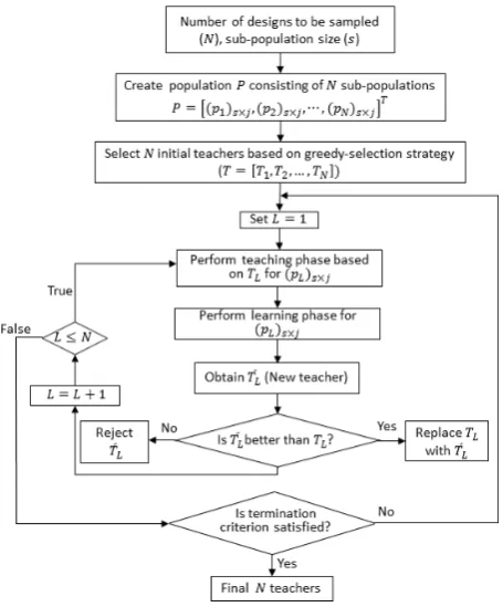
T are updated after each sub-iteration for the sub-population. The teacher is a learner having a minimum cost value (computed with the teachers of other sub-populations) among the other learners in the same sub-population. Sub-iterations in other sub-populations are performed in the same way. S-TLBO is terminated when change in the cost values after two consecutive iterations performed in the population become negligibly small. Figure 2 shows the flow chart for the S-TLBO algorithm.

Figure 2: Flow chart of S-TLBO

3.2. Sampling designs with S-TLBO in unconstrained spaces

U1(T)=

N−1 X

p=1

N

X

q=p+1

1 Pn

j₌1(xp,j−xq,j)2

(6)

xp,jandxq,jare thescaledparameter values for the jth subject (dimension) of the teachers (designs)pandq in

T which are computed by scaling parameter values between 0 (i.e., lower bound for the parameter) and 1 (i.e., upper bound for the parameter). These bounds form the design space, which is calledscaled design space. Recall thatN

is the number of designs to be sampled andnis the number of dimensions in the design space. The potential energy in Equation (6) has to be minimized. Figure 3 (a) shows 25 samples (i.e.,N =25) generated using Equation (6) for a two-dimensional problem. It is seen that samples spread evenly in the design space, therefore space-filling designs can be obtained.

Figure 3: (a) Space-filling designs (b) Non-collapsing designs (c) Space-filling and non-collapsing designs.

Minimization of the potential energyU1(T) favors placement of the designs at the maximum separating distance from each other. However, this energy function itself locates designs at the corners and on the boundaries of the design space particularly for the high-dimensional sampling problems [5]. For the CAD model sampling, it is desired to spread designs evenly also in the inner portions of the design space. Therefore, non-collapsing property (i.e., designs not sharing same parameter values) for the sampled designs should be satisfied as much as possible. Figure 3 (a) and (b) show collapsing and collapsing designs, respectively. Sampling designs with only considering non-collapsing property for the constrained design spaces may result in designs with poor space-filling property as seen in Figure 3 (b). When both space-filling and non-collapsing properties are considered, better sampling can be achieved (see Figure 3 (c)). Note that the samples in Figure 3 are obtained using the S-TLBO approach withN=25 ands=10. A penalization technique is introduced in order to sample non-collapsing designs in the design space. A new term,

U2(T), is included in the cost function, which is as follows:

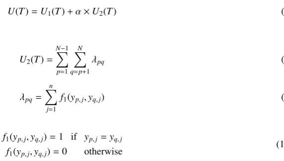
U(T)=U1(T)+α×U2(T) (7)

where

U2(T)=

N−1 X

p=1

N

X

q=p+1

λpq (8)

λpq= n

X

j=1

f1(yp,j,yq,j) (9)

f1(yp,j,yq,j)=1 if yp,j=yq,j

f1(yp,j,yq,j)=0 otherwise

(10)

αis a user-defined parameter adjusting weight for the U2(T) term. The parameter values for designs are first converted into integer values. yp,j andyq,j in Equation (9) are the corresponding integer coordinate values for xp,j

and xq,j in the jth dimension (subject), respectively. λpq denotes the number of coordinates that two designs, p

andq share. The range of each design parameter is partitioned into N equal intervals (levels) as follows: [xl m,j =

x1

m,j,x

2

m,j, . . . ,x N m,j = x

u

integer number varying from 1 toN. λpq for the designspandqis then computed using the piecewise function f1 shown in Equation (10).

if xr_p,j≤xp,j<xrp+,1j then yp,j=r

if xr_q,j≤xq,j<xqr+,j1 then yq,j=r

with 1≤r≤N

(11)

The termU2(T) is based on the degree of violation for the non-collapsing property. Maximum value for this term can be j×N_C

2. NC2 represents the combinations between designs which is as follows: NC2 = _2!(NN₋!_2)!. Setting the parameterαto larger values will lead to producing more non-collapsing designs. On the other hand, the designs sampled may have poor space-filling as seen in Figure 3 (b). As a result,αshould be tuned carefully which will be discussed in the ”Results and Discussion” section.

3.3. Sampling designs with S-TLBO in constrained spaces

Design space consists of feasible and infeasible regions in the case of constrained spaces. Feasible regions con-sist of feasible designs that satisfy the predefined design constraints. Infeasible designs are located in the infeasible regions. We transform the constrained problem to an unconstrained one by using a static constraint handling mech-anism. This concept was introduced in genetic algorithms by Homaifar et al. [30] and has been utilized in many works [52, 53, 54, 55]. In this mechanism, designs are penalized if they violate any constraint. The cost function

U(T) is utilized for constrained spaces which is written below:

U(T)=U(T)+β×U3(T) (12)

where

U3(T)=

N

X

p=1

nc

X

t=1

f2(p,t) (13)

f2(p,t)=1 if the constraintφtis violated by the design p

f2(p,t)=0 otherwise

(14)

The cost functionU(T) consists of the termsU(T),U3(T) and a parameter,βthat adjusts the weight ofU3(T). Let

ncbe the number of geometric constraints andφtrepresent a constraint, wheret=1, . . . ,nc. The piecewise function

f2gets a value of 1 if a design,p, violates the constraintφt(see Equation (14)). Otherwise, it is 0. The termU3(T) is computed using Equation (13).

The cost functionU(T) is overall composed of three terms,U1(T),U2(T) andU3(T) and two parameters;αand

β, which is shown below:

U(T)=

N−1 X

p=1

N

X

q=p+1

1 Pn

j=1(xp,j−xq,j)2 +

α×

N

X

p=1

N

X

q=p+1

λpq + β× N

X

p=1

nc

X

t=1

f2(p,t)

(15)

Figure 4: CAD model of a yacht hull (a), a sherry-type wine glass without base (glass-1) (b), a pinot noir-type wine glass (glass-2) (c) and a wheel rim (d) with their design parameters.

4. CAD Models for Study’s Experiments

S-TLBO can generate a variety of designs for a given CAD model in the constrained and unconstrained design spaces. Both the design specifications and user preferences can be represented by constraints. To validate the per-formance of S-TLBO, four different CAD models were utilized, as follows: a yacht hull, wheel rim, sherry-type wine glass without a base (glass-1), and pinot noir-type wine glass (glass-2). These models are shown in Figure 4. The constraints for the yacht hull and glass-1 models were formulated by incorporating the user preferences. For the glass-2 model, the design specifications, such as the glasss capacity to store a certain amount of liquid, were given as constraints. The constraints for the yacht hull and glass-1 models were determined via one-to-one interviews with the participants; thus, to some extent, they reflect customer preferences related to the product. We call this

customer-centered design sampling. A customer-centered design is developed considering the customers perspectives by understanding their preferences [56, 57, 58]. The design sampling is first carried out without constraints, and the sampled designs are shown to the participants to learn their preferences. By including these preferences as S-TLBO constraints, sampling can be performed in the constrained space.

For higher design variations, we divided the yacht hull model into three regions, as follows: the entrance, middle, and run. The glass-1 model had lower and upper regions, while the profiles of the wheel rim and glass-2 models were divided into three curves. The 3Dsurface models for these models were obtained by lofting between the Bezier curves separately in each region, and the design parameters were defined on the curves. The surface modification of the models was performed using the technique proposed by Khan et al. [59]. The design parametersLe,Lm, andLr

represent the lengths of the entrance, middle, and run regions, respectively, of the yacht hull. Moreover,Be,Bm,Brand

De,Dm,Drdenote the beams and widths of regions, respectively, whileθis the entrance angle andβis the bow angle.

For the glass-1 model, the heights of the lower and upper regions are denoted byHlandHu, respectively. Moreover,

WlandWuare the widths of the lower and upper regions, respectively, whileWmdenotes the width at the connection

the design parameters) that were used in this study’s experiments for the yacht hull, glass, and wheel rim models, respectively.

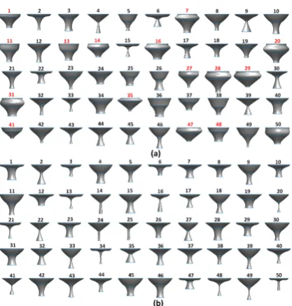
The design constraints for the yacht hull and glass-1 can be seen in Tables 1 and 2, respectively. S-TLBO first sampled designs in an unconstrained space; following this, participants’ preferences concerning the appearance of these designs were learned via comprehensive one-to-one interviews. There were 30 and 50 samples obtained for the yacht hull and glass-1 models, respectively, as shown in Figures 5 (a) and 6 (a). Three participants attended the interview for the yacht hull model, whereas only one participant was interviewed for the glass-1 model. The CAD models generated by S-TLBO were shown to the participants one by one to learn whether they liked or disliked the models. Next, they were asked about the reasons for their preferences concerning the models. The following questions were asked when a model was shown to the participants:

• Familiarize yourself with this model by viewing it from different perspectives.

• Do you like or dislike it?

• If you like it, which features of this model do you like?

• If you dislike it, which features of this model do you dislike?

In this way, the participants’ preferences were quantized and represented by geometric constraints. For instance, the participant disliked the designs in Figure 6 (a), numbered in red as 1, 7, 11, 13, 14, 16, 20, 27, 28, 29, 31, 35, 41, 47, 48, and 50. When these models are visually inspected, it can be recognized that the parameterWmis approximately equal

to or higher thanWu. The participant preferred designs withWuparameter values of at least twice theWmparameter

values. As the objective of this study was to perform sampling in a predetermined design space, the constraints in Tables 1 and 2 are not all explained here in detail. Based on the predetermined constraints, S-TLBO was utilized once again in constrained design spaces for the generation of customer-centered designs.

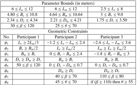
Table 1: Parameter bounds and geometric constraints for the yacht hull model

Parameter Bounds (in meters)

6≤Le≤12 6≤Lm≤12 2.5≤Lr≤8

4.80≤Be≤10.8 4.64≤Bm≤10.64 3≤Br≤9.0

2.34≤De≤4.34 2.21≤Dm≤4.21 1.75≤Dr≤3.50

30≤β≤120 25≤θ≤70

Geometric Constraints

No. Participant 1 Participant 2 Participant 3

φ1 Lr ≥2Lm/3 −1.2≤Le−Lm≤2.4 −2.4≤Le−Lm≤3.6 φ2 Be≥Bm/2 Lr≥Lm/2 Lm≥Lr≥Lm/2 φ3 Bm≥Br 0≤Be−Bm≤2.4 −1.8≤Be−Bm≤3 φ4 De≥Dm≥Dr Bm≥Br Bm≥Br φ5 50≤β≤120 0≤De−Dm≤0.7 0≤De−Dm≤0.7

φ6 Dm≥Dr Dm≥Dr

φ7 40≤β≤70 110≤β≤80

φ8 45≤θ≤70 if (β≥110) thenθ≥55

5. Results and Discussion

Figure 5: (a) Designs obtained using S-TLBO without the geometric constraints. Designs obtained with the geometric constraints, quantified for participants 1 (b), 2 (c) and 3 (d) for the yacht hull model. (The participants disliked the designs numbered in red).

Figure 6: Designs obtained using S-TLBO without (a) and with (b) the geometric constraints quantified for the participant for the glass-1 model. (The participant disliked the designs numbered in red).

Figure 7: Glass-2 designs obtained using S-TLBO without (a) and with (b) the geometric constraint.

Figure 8: Designs obtained for the wheel rim models using S-TLBO.

5.1. Computational Time

Table 2: Parameter bounds and geometric constraints for glass-1 and glass-2

Wine Glass-1 Wine Glass-2

Parameter Bounds (in millimeters)

40≤Hu≤120 90≤Hl≤170 50≤H0≤100 90≤H1≤115

130≤Wu≤170 15≤Wm≤160 130≤H2≤155 175≤H3≤200

15≤Wl≤65 17.5≤W1≤60 37.5≤W2≤60

32.5≤W3≤60

Geometric Constraints

φ1 Hl≥Hu volume ≤ 200

φ2 Wm≤Wu/2

φ3 Wm≤Wl

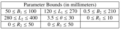
Table 3: Parameter bounds for the wheel rim model

Parameter Bounds (in millimeters)

50≤B1≤100 120≤L1≤270 0.5≤B2≤210

280≤L2≤400 3.5≤θ≤30 0≤R1≤10

0≤R2≤50 0≤R3≤50

be sampled (N), dimensionality of the design space (n), and size of the subpopulations (s). Increases in the values of these parameters will increase the S-TLBO’s processing time. Due to the larger value of s, the sampled designs in Figure 5 (d) had the highest computational time compared with the sampled designs in Figure 5 (a), (b), and (c). Furthermore, S-TLBO takes more time when it is used in constrained spaces. For instance, the designs in Figure 5 (b) were obtained after a higher processing time of S-TLBO than those obtained in Figure 5 (a), even with the same parameter settings forN,n, ands. The computational complexity of TLBO for a single iteration isO(s·n). Since S-TLBO hasNsubpopulations, its computational complexity for a single iteration isO(s·n·N). Letimaxbe the total

number of iterations after the termination of S-TLBO; the computational complexity of S-TLBO isO(s·n·N,imax).

Table 4: Processing time taken to obtain the sampling results in Figures 5, 6, 8, and 11

N n s U(T) U1(T) Number of Collapsing Models Computational Time (minute)

Results in Figure 5 (a) 30 11 60 241.78 245.31 0 16.08

Results in Figure 5 (b) 30 11 60 23113.49 269.62 16 16.46

Results in Figure 5 (c) 30 11 70 13127.32 261.00 18 21.50

Results in Figure 5 (d) 30 11 80 11111.18 250.61 16 29.36

Results in Figure 6 (a) 50 5 30 1885.94 1734.16 0 10.63

Results in Figure 6 (b) 50 5 30 6757.20 2071.37 30 10.91

Results in Figure 7 (a) 20 7 20 167.04 137.85 20 3.60

Results in Figure 7 (b) 10 7 20 372.22 42.22 10 1.73

Results in Figure 8 10 8 20 28.91 30.62 0 3.28

Results in Figure 11 30 11 – – 421.86 28 2.58

5.2. Algorithm Convergence

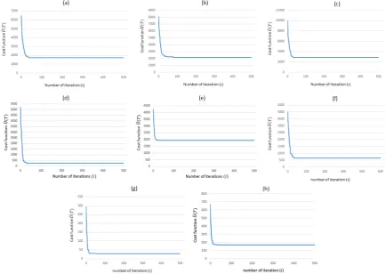
the designs in Figures 5, 6, 7, and 8. Many iterations were performed for the models in Figures 5, 6, 7, and 8 to analyze the convergence of the S-TLBO algorithm (see the plots in Figure 9). No improvements were observed in the cost function (U(T)) after some consecutive iterations. There was no change in the cost function after approximately the 60th_{iteration for the models in Figures 5 (a), 5 (d), 5 (c), 6, 7, and 8. For the models in Figure 5 (b), S-TLBO}

converged ati=80. The convergence rate depends on the number of designs that are sampled (N), dimensionality of design space (n), and total number of constraints (nc). Due to its low dimensionality and the presence of fewer

geometric constraints, S-TLBO converges faster for the sampling problem in Figure 6 than that in Figure 5.

Figure 9: (a), (b), (c), (d) Plots showing the cost value versus number of S-TLBO iterations for the models in Figure 5 (a), (b), (c), and (d), respectively. (e), (f), (g), (h) Plots showing the cost value versus number of S-TLBO iterations for the models in Figures 6 (a), 6 (b), 8, and 7 (a), respectively.

5.3. Comparison with Existing Works

We compared the performance of S-TLBO with the existing state-of-the-art techniques in the literature that have been proposed to generate optimal space-filling designs in experiments. First, we compared the performance of S-TLBO with Fuerle and Sienz’s [4] technique. For the comparison, we utilized the two-dimensional examples 2 and 7 in the paper [4], which are also shown in Figure 10 (a) and (c), respectively. Examples 2 and 7 utilize Equations 16 and 17, respectively, as constraints.

(x1−0.5)2+(x2−0.5)2≥0.25

0≤x1≤1

0≤x2≤1

(x1−0.5)2+(x2−0.5)2 ≥0.1

(x1)2+(x2−1)2≥1/3

(x1−1)2+(x2)2≥1/3

0≤x1≤1

0≤x2≤1

(17)

Fifteen design points (i.e., N = 15) were sampled under the above constraints via S-TLBO. These points are shown in Figure 10 (b) and (d), which are plotted after conversion into integer coordinates using Equation 11. The designs in Figure 10 (b) were obtained with theα =50,β= 2000, ands =40 settings. The designs in Figure 10 (d) were obtained with the following settings:α=30,β=2000, ands=40. The sampled designs generated using Fuerle and Sienz’s [4] method are shown in Figure 10 (a) and (c). The values of potential energyU1(T) for the design points in Figure 10 (a), (b), (c), and (d) are were about 610, 555, 618, and 518, respectively. The potential energies of the sampled design points generated by S-TLBO were lower than those produced by Fuerle and Sienz’s technique.

Figure 10: Design points are generated based on the constraints defined in Equation 16 using (a) Fuerle and Sienz’s [4] technique and (b) S-TLBO. The design points are obtained based on the constraints defined in Equation 17 using (c) Fuerle and Sienz’s [4] method and (d) S-TLBO (images (a) and (c) are taken from [4]).

We also compared the performance of S-TLBO with random sampling and other techniques, such as the Lp

optimization technique proposed by Torsset [15], recently proposed CoNcaD technique of Dragulji´c et al. [17], and NPL algorithms SFDP* and SFDP** proposed by Stinstra et al. [13]. These techniques utilized themaximin distance

proposed by Johnson et al. [10] for creating space-filling designs (see Equation 18). Therefore, we used Equation 18 instead of Equation 6 to allow comparison of our work with these methods. Equation 18 spreads out the designs in the design space by maximizing the minimum interpoint distance between the pair of designs, which is expressed as follows:

max

T Xpmin,Xq∈T

v

t n

X

j=1

(xp,j−xq,j)2 (18)

The quadrant/ball region example was also tested; this was defined by the following constraints: xj ≥0 where

j = 1,2, . . . ,nandPn j=1(x

2

j) ≤ 0. Forn =2 andn = 10, the designs were obtained using S-TLBO’s constrained

formulation with the maximin distance in Equation 18 for the settings ofα=0,β=2000, andi=500. Table 5 shows the maximin distances for the design points produced byLpoptimization, SFDP* and SFDP**, CoNcaD , and random

sampling, S-TLBO, and S-TLBO (α = 0) . To compare the S-TLBO results with those of random sampling for the quadrant/ball region example, the designs were randomly selected from the design space. The samples violating the constraint(s) were rejected, and random sampling was repeated until allN samples satisfied the constraints. As mentioned in [13], SFDP* cannot be used for sampling problems with a high number of constraints. As shown in Table 5, except forn=10 andN=10, the design points generated by S-TLBO have a higher maximin distance value (i.e., better sampling quality) than those produced by the SFDP** and CoNcaD techniques. It should be noted that random sampling andLpproduced the poorest results compared with the other techniques. Especially,Lpgenerated

the worst samples in high-dimensional design spaces (i.e.,n =10). According to the experiments, we observed that S-TLBO generated samples with better sampling quality, especially for large values ofnandN. It is noteworthy that SFDP* and SFDP** do not consider the non-collapsing property during sampling, and therefore, these techniques should also be compared with S-TLBO when the parameterα is set to zero. In Table 5, S-TLBO (α = 0) is the S-TLBO algorithm whenα=0. It is shown in Table 5 that S-TLBO (α=0) produces better results than SFDP* and SFDP**.

Table 5: The maximin distance (in Equation 6) of the designs produced by different algorithms forn =2 andn=10 using the quadrant/ball example (NA: Not Applicable)

n N Random Sampling SFDP* SFDP** LP CoNcaD S-TLBO S-TLBO(α=0)

2 10 0.0444 0.3587 0.3522 0.2554 0.3400 0.3565 0.3630

2 20 0.0537 0.2394 0.1966 0.2212 0.2124 0.2292 0.2391

2 50 0.0063 0.1403 0.1188 0.1336 0.1204 0.1283 0.1409

2 100 0.0046 NA 0.0486 0.0660 0.0789 0.0822 0.0893

2 200 0.0037 NA 0.0259 0.0070 0.0539 0.0566 0.0584

10 10 0.3606 1.4142 1.2167 0.5017 1.3027 1.0882 1.4358

10 20 0.3095 1.0323 0.9591 0.4138 0.8364 0.9877 1.0461

10 50 0.2658 0.8811 0.7588 0.2952 0.6747 0.7917 0.8852

10 100 0.2203 NA 0.6248 0.2753 0.5838 0.6770 0.7095

10 200 0.1367 NA 0.5235 0.2559 0.5160 0.5689 0.5817

To compare the results of S-TLBO with random sampling, we generated the yacht hull model in Figure 4 (a) via random sampling under the constraints quantified from participant 1. Thirty yacht hull models were generated via random sampling. A model violating the constraint(s) was rejected, and a new model was sampled. The sampling was repeated until all 30 models satisfying the constraints were obtained, as shown in Figure 11. These 30 randomly sampled models were compared with the models in Figure 5. It can be seen from Table 4 that the random sampled models have a poorer space-filling property than those obtained from S-TLBO.

5.3.1. Statistical Analysis of Results in Table 5

We also analyzed the statistical performance of the proposed approach over the other techniques in Table 5. The Shapiro-Wilk and Kolmogorov-Smirnov normality tests were performed to check the distribution of the data in the table 5. The significance values for these tests were smaller than 0.05, which implies that the data have a non-normal distribution. The histogram plot in Figure 12 also confirmed this, which is obtained using the results of the proposed and benchmark techniques in Table 5. The data distribution is left-skewed with a skewness value of 1.032, therefore the data have a non-normal distribution. Thus, the Friedman test [60], a nonparametric statistical test, was used. It should be noted that the nonparametric approaches have been employed by researchers to compare the performance of swarm and evolutionary algorithms [61, 62, 63].

Figure 11: Yacht hull models generated via random sampling under the constraints quantified from participant 1

Figure 12: Histogram plot for the data in Table 5

in Table 5 were not provided due to the incapability of SFDP*.

respectively, for the second dataset. The criticalchi2 was 12.59 for both datasets. As the p-values were less than 0.05, and thechi2values were greater than the criticalchi2(12.59), these results indicated strong evidence againstH0. Similarly, the results showed strong evidence againstH0 for the pairwise comparison.

Furthermore, pairwise comparison analyses were also performed for the first and second datasets, and their results can be seen in Tables 6 and 7, respectively. It should be noted that only S-TLBO and CoNCaD consider the non-collapsing criterion. Therefore, results of these techniques should be compared. On the other side, the results of random sampling, SFDP*, SFDP** andLp should be compared with S-TLBO (α = 0) as these techniques do not

consider the non-collapsing criterion. The computed p-values for S-TLBO-CoNcaD and S-TLBO(α = 0)-others (others include random, SFDP*, SFDP ** and Lp) are all less than 0.05, and the chi2 values are greater than the criticalchi2(3.84) in Table 6. This proves that the null hypothesisH0 is rejected for the present analysis. Similarly, the computedp- andchi2values for S-TLBO-CoNcaD and S-TLBO(α=0)-others in the second dataset are shown in Table 7, which are again less than 0.05 and the criticalchi2value, respectively. These results imply that the null hypothesis H0 is rejected. This concludes that the results shown in Table 5 obtained using S-TLBO are significantly different from those obtained using the other alternative techniques. Consequently, S-LTBO has statistically better performance (i.e., space-fillingness) than the other alternative techniques.

Consequently, the Friedman test shows that the results given in Table 5 obtained using S-TLBO are significantly different from those obtained using the other alternative techniques. As S-TLBO has better performance (i.e. better space-filling property) according to the experiments in Table 5, it can be concluded that S-TLBO has statistically better performance than the other alternative techniques.

Table 6:p-values andchi2_{values for the first dataset obtained from the Friedman test in pairwise comparison}

Random Sampling SFDP** Lp CoNcaD S-TLBO S-TLBO (α=0)

p-values

Random Sampling NaN 0.001 0.001 0.001 0.001 0.001

SFDP** 0.001 NaN 0.205 1 0.011 0.001

Lp 0.001 0.205 NaN 0.057 0.011 0.001

CoNcaD 0.001 1 0.057 NaN 0.011 0.001

S-TLBO 0.001 0.011 0.011 0.011 NaN 0.001

S-TLBO(α=0) 0.001 0.001 0.001 0.001 0.001 NaN

chi2values

Random Sampling NaN 10 10 10 10 10

SFDP** 10 NaN 1.6 0 6.4 10

Lp 10 1.6 NaN 3.6 6.4 10

CoNcaD 10 0 3.6 NaN 6.4 10

S-TLBO 10 6.4 6.4 6.4 NaN 10

S-TLBO(α=0) 10 10 10 10 10 NaN

5.3.2. Comparison of S-TLBO with NSGA-II’s non-dominated sorting and crowding distance phenomenon

We compared the weighted combination of objectives (U1(T), U2(T), and U3(T)) with nonparameterized ap-proaches, such as NSGA-II [64], which relies on the Pareto dominance and crowding distance to prioritize solutions. Zou et al. [65] proposed an improved TLBO called multi-objective teaching-learning-based optimization (MOTLBO). In MOTLBO, Zou et al. [65] used an external archive to retain the best solutions. The concept of nondominated sorting and the mechanism of crowding distance computation are incorporated into the algorithm, specifically in the teacher phase. Like in Zou et al.s [65] work, we incorporated the nondominated sorting concept and mechanism of crowding distance in S-TLBO, and we call the revised approach S-TLBO*.

Table 7:p-values andchi2_{values for the second dataset obtained from the Friedman test in pairwise comparison}

Random Sampling SFDP* SFDP** Lp CoNcaD S-TLBO S-TLBO (α=0)

p-values

Random Sampling NaN 0.527 0.001 0.001 0.001 0.001 0.001

SFDP* 0.527 NaN 0.527 0.527 0.527 0.527 0.011

SFDP** 0.001 0.527 NaN 0.205 1 0.011 0.001

Lp 0.001 0.527 0.205 NaN 0.057 0.011 0.001

CoNcaD 0.001 0.527 1 0.057 NaN 0.011 0.001

S-TLBO 0.001 0.527 0.011 0.011 0.011 NaN 0.001

S-TLBO (α=0) 0.001 0.011 0.001 0.001 0.001 0.001 NaN

chi2values

Random Sampling NaN 0.4 10 10 10 10 10

SFDP* 0.4 NaN 0.4 0.4 0.4 0.4 6.4

SFDP** 10 0.4 NaN 1.6 0 6.4 10

Lp 10 0.4 1.6 NaN 3.6 6.4 10

CoNcaD 10 0.4 0 3.6 NaN 6.4 10

S-TLBO 10 0.4 6.4 6.4 6.4 NaN 10

S-TLBO (α=0) 10 6.4 10 10 10 10 NaN

2ssolutions based on the nondominated sorting and crowding distance for the next generation. In S-TLBO*, each initial teacher is selected from its external archive, and a nondominated solution in the first Pareto front can be used as the teacher. If there are two or more nondominated solutions in the first Pareto front, then the solution with the highest crowding distance value is selected as the teacher.

A solutionX1is said to be Pareto dominated by the other solution X2ifU1(X1)≤U1(X2)∧U2(X1)≤U2(X2)∧

U3(X1)≤U3(X2) andU1(X1)<U1(X2)∨U2(X1)<U2(X2)∧U3(X1)<U3(X2). This dominating criterion is initiated to make designs that guarantee the validation of the geometric constraints in each iteration. During the teacher and learner phases, a new learner, X0₁, replaces the previous learnerX1 ifX₁0 dominates X1. Moreover,X₁0 is rejected if

X1dominates. WhenX0₁andX1do not dominate each other, we randomly select one to add to the population. As in S-TLBO, teachers are selected as the sampled designs at the end of the last iteration.

The performance of S-TLBO* was compared with that of S-TLBO for the wheel rim, glass-1, and yacht hull models for the settings ofi=30,s=10, andN =10. Table 8 shows that the values ofU1(T) for the wheel rim and yacht samples in the case of S-TLBO were lower than those obtained using S-TLBO*. For all the test models, the values ofU2(T) andU3(T) for the samples obtained using S-TLBO were less than those generated by S-TLBO*. The computational cost of S-TLBO* is approximately two times higher than that of S-TLBO.

5.4. User Study

Table 8: Comparison of S-TLBO with S-TLBO* for the wheel rim, glass, and yacht hull models.

Wheel Rim Wine Glass Yacht Hull

STLBO

U1(T) 28.70 58.90 22.40

U2(T) 0 9 8

U3(T) – 0 0

Computational Time (minutes) 3.28 1.72 3.09

S-TLBO*

U1(T) 33.34 56.20 29.20

U2(T) 36 13 34

U3(T) – 12 15

Computational Time (minutes) 7.38 3.83 5.95

Figure 13: Glass-2 models generated using random sampling.

At-test was also utilized to statistically examine the S-LTBO performance. The users data were normally dis-tributed, as the skewness value was close to zero, and their mean/median values were approximately equal. The null hypothesis states that the ratings given to the designs generated using random sampling and S-LTBO will be similar. The p-value obtained from the t-test was less than the significance level of 0.05, so the null hypothesis was rejected.

5.5. Parameter Tuning

S-TLBO utilizes the static constraint handling method to favor the sampling of feasible designs. Here, βis a parameter in the cost functionU(T) that adjusts the weight of the term U3(T), while αis a parameter in the cost functionU(T) that adjusts the weight of the term U2(T). Experiments were conducted to observe the behavior of S-TLBO at different values ofα.

Figure 14 (a), (b), and (c) show plots of the number of designs violating the geometric constraints versusβfor the yacht hull model for participants 1, 2, and 3. Figure 14 (d) shows a plot for the number of designs violating the geometric constraints versusβfor the glass-1 model. No generated CAD models violated any design constraint when parameterβwas set to values greater than 600. Therefore,βwas set to 2,000 in this study’s experiments. Figure 15 (a) and (b) show plots of the number of collapsing designs versusα. There were 49 collapsing designs whenαwas set to 0. Whenαincreased, the number of collapsing designs decreased, and this reached zero whenα=40. Therefore,

αwas set to 100 in this study, except for the designs in Figure 7.

A 3Dsurface plot, shown in Figure 16, was also obtained to validate the ideal values forαandβ. It can be observed that the value ofU1(T) was minimal whenαandβwere equal to zero. Whenαwas zero, most of the sampled designs were collapsing, and thus, they spread more uniformly in the design space. Whenαincreased, the sampled designs tended to be non-collapsing, and therefore,U1(T) increased. According to the plot,U1(T) started to increase rapidly untilα =40; after this point, it became almost constant. A similar trend was observed for the parameterβ. When

Table 9: Results of the second user study

Random Sampling S-TLBO

User Average Grade

1 2.85 3.50

2 3.65 4.15

3 3.75 4.40

4 2.65 4.30

5 2.25 2.55

6 3.10 2.70

7 4.15 3.85

8 3.45 3.55

9 4.15 3.85

10 3.15 2.9

11 2.85 3.20

12 2.60 2.80

13 3.35 3.55

14 2.70 3.00

U1(T) 226.23 137.84

U2(T) 88.00 32.00

σ 1.024 1.070

µ 3.190 3.450

Median 3.00 3.00

S kewness -0.04 -0.180

p-value 0.003365

The size of the subpopulations (s) also plays an important role for the generation of space-filling designs. Higher values ofscreate a diverse initial solution for S-TLBO, which facilitates its search of the design space for the global optimum solution. In contrast, the application of S-TLBO with higher values ofscan result in a higher computational cost. We recommend setting sto a value higher than 20. Table 4 provides values of s, U(T), and the number of collapsing designs for the designs in Figures 5, 6, 7, 8, and 11.

6. Conclusions and Future Works

This paper proposes a sampling method for CAD models. Teaching-Learning-Based Optimization (TLBO) is extended for design sampling in constrained and unconstrained spaces. The S-TLBO approach randomly generates sub-populations and improves learners in these sub-populations using teaching and learning phases. To obtain distinct designs in the design space, designs with space-filling and non-collapsing properties are favored during sampling. Designs, that do not satisfy predefined design constraints are penalized using a constraint handling mechanism. After S-TLBO terminates, teachers of sub-populations are regarded as the sampled designs.

Figure 14: (a), (b), (c), (d) Plots showing the number of designs violating the geometric constraints versusβfor the models in Figures 5 (b), (c), and (d) and 6 (b), respectively.

Figure 15: Plot of the number of collapsing designs versusαwhenβ=0 (a) andβ=2,000 (b).

Acknowledgment

This work is supported by the Scientific and Technological Research Council of Turkey (Project Number: 214M333). The authors would like to thank Dr. Serkan Gunpinar and Mr. Kemal Mert Dogan for their help about statistical anal-ysis.

References

[1] I. Kaymaz, C. A. McMahon, A response surface method based on weighted regression for structural reliability analysis, Probabilistic Engi-neering Mechanics 20 (1) (2005) 11–17.

[2] P. Audze, V. Eglais, New approach for planning out of experiments, Problems of dynamics and strengths 35 (1977) 104–107.

[3] R. Lekivetz, B. Jones, Fast flexible space-filling designs for nonrectangular regions, Quality and Reliability Engineering International 31 (5) (2015) 829–837.

[4] F. Fuerle, J. Sienz, Formulation of the audze–eglais uniform latin hypercube design of experiments for constrained design spaces, Advances in Engineering Software 42 (9) (2011) 680–689.

[5] V. R. Joseph, E. Gul, Maximum projection designs for computer experiments, Biometrika 102 (2) (2015) 371–380.

Figure 16: Surface plot ofU1(T) versusβversusα.

[7] G. Damblin, M. Couplet, B. Iooss, Numerical studies of space-filling designs: optimization of latin hypercube samples and subprojection properties, Journal of Simulation 7 (4) (2013) 276–289.

[8] B. G. Husslage, G. Rennen, E. R. van Dam, D. den Hertog, Space-filling latin hypercube designs for computer experiments, Optimization and Engineering 12 (4) (2011) 611–630.

[9] P. Z. Qian, C. J. Wu, Sliced space-filling designs, Biometrika (2009) 945–956.

[10] M. E. Johnson, L. M. Moore, D. Ylvisaker, Minimax and maximin distance designs, Journal of statistical planning and inference 26 (2) (1990) 131–148.

[11] T. M. Cioppa, T. W. Lucas, Efficient nearly orthogonal and space-filling latin hypercubes, Technometrics 49 (1) (2007) 45–55. [12] M. C. Shewry, H. P. Wynn, Maximum entropy sampling, Journal of applied statistics 14 (2) (1987) 165–170.

[13] E. Stinstra, D. den Hertog, P. Stehouwer, A. Vestjens, Constrained maximin designs for computer experiments, Technometrics 45 (4) (2003) 340–346.

[14] E. Benkov´a, R. Harman, W. G. M¨uller, Privacy sets for constrained space-filling, Journal of Statistical Planning and Inference 171 (2016) 1–9.

[15] M. W. Trosset, Approximate maximin distance designs, in: Proceedings of the Section on Physical and Engineering Sciences, 1999, pp. 223–227.

[16] M. D. McKay, R. J. Beckman, W. J. Conover, A comparison of three methods for selecting values of input variables in the analysis of output from a computer code, Technometrics 42 (1) (2000) 55–61.

[17] D. Dragulji´c, T. J. Santner, A. M. Dean, Noncollapsing space-filling designs for bounded nonrectangular regions, Technometrics 54 (2) (2012) 169–178.

[18] A. Grosso, A. Jamali, M. Locatelli, Finding maximin latin hypercube designs by iterated local search heuristics, European Journal of Opera-tional Research 197 (2) (2009) 541–547.

[19] M. Petelet, B. Iooss, O. Asserin, A. Loredo, Latin hypercube sampling with inequality constraints, AStA Advances in Statistical Analysis 94 (4) (2010) 325–339.

[20] P. Prescott, Orthogonal-column latin hypercube designs with small samples, Computational Statistics & Data Analysis 53 (4) (2009) 1191– 1200.

[21] S. J. Bates, J. Sienz, D. S. Langley, Formulation of the audze–eglais uniform latin hypercube design of experiments, Advances in Engineering Software 34 (8) (2003) 493–506.

[22] R. V. Rao, V. J. Savsani, D. Vakharia, Teaching–learning-based optimization: a novel method for constrained mechanical design optimization problems, Computer-Aided Design 43 (3) (2011) 303–315.

[23] R. V. Rao, Teaching learning based optimization algorithm and its engineering applications, Springer International Publishing, Switzerland, 2016.

[24] J. H. Holland, Adaptation in natural and artificial systems: an introductory analysis with applications to biology, control, and artificial intelligence, MIT press, 1992.

[25] R. Poli, J. Kennedy, T. Blackwell, Particle swarm optimization, Swarm intelligence 1 (1) (2007) 33–57.

[26] D. Karaboga, B. Basturk, On the performance of artificial bee colony (abc) algorithm, Applied soft computing 8 (1) (2008) 687–697. [27] R. Storn, K. Price, Differential evolution–a simple and efficient heuristic for global optimization over continuous spaces, Journal of global

optimization 11 (4) (1997) 341–359.

Interna-tional Conference on Frontiers of Intelligent Computing: Theory and Applications (FICTA), Advances in Intelligent Systems and Computing, Vol. 199, Springer, 2013, pp. 395–403.

[30] A. Homaifar, C. X. Qi, S. H. Lai, Constrained optimization via genetic algorithms, Simulation 62 (4) (1994) 242–253.

[31] R. Rao, V. Patel, An elitist teaching-learning-based optimization algorithm for solving complex constrained optimization problems, Interna-tional Journal of Industrial Engineering Computations 3 (4) (2012) 535–560.

[32] S. C. Satapathy, A. Naik, K. Parvathi, A teaching learning based optimization based on orthogonal design for solving global optimization problems, SpringerPlus 2 (1) (2013) 130.

[33] D. Chen, F. Zou, Z. Li, J. Wang, S. Li, An improved teaching–learning-based optimization algorithm for solving global optimization problem, Information Sciences 297 (2015) 171–190.

[34] H.-b. Ouyang, L.-q. Gao, X.-y. Kong, D.-x. Zou, S. Li, Teaching-learning based optimization with global crossover for global optimization problems, Applied Mathematics and Computation 265 (2015) 533–556.

[35] R. Rao, V. Patel, A multi-objective improved teaching-learning based optimization algorithm for unconstrained and constrained optimization problems, International Journal of Industrial Engineering Computations 5 (1) (2014) 1–22.

[36] K. Yu, X. Wang, Z. Wang, Constrained optimization based on improved teaching–learning-based optimization algorithm, Information Sci-ences 352 (2016) 61–78.

[37] S. C. Satapathy, A. Naik, Data clustering based on teaching-learning-based optimization, in: International Conference on Swarm, Evolution-ary, and Memetic Computing, Springer, 2011, pp. 148–156.

[38] S. C. Satapathy, A. Naik, K. Parvathi, Unsupervised feature selection using rough set and teaching learning-based optimisation, International Journal of Artificial intelligence and Soft Computing 3 (3) (2013) 244–256.

[39] Y. Xu, L. Wang, S.-y. Wang, M. Liu, An effective teaching–learning-based optimization algorithm for the flexible job-shop scheduling problem with fuzzy processing time, Neurocomputing 148 (2015) 260–268.

[40] A. Baykaso˘glu, A. Hamzadayi, S. Y. K¨ose, Testing the performance of teaching–learning based optimization (tlbo) algorithm on combinatorial problems: Flow shop and job shop scheduling cases, Information Sciences 276 (2014) 204–218.

[41] Z. Xie, C. Zhang, X. Shao, W. Lin, H. Zhu, An effective hybrid teaching–learning-based optimization algorithm for permutation flow shop scheduling problem, Advances in Engineering Software 77 (2014) 35–47.

[42] J. Zhou, X. Yao, Hybrid teaching–learning-based optimization of correlation-aware service composition in cloud manufacturing, The Inter-national Journal of Advanced Manufacturing Technology (2017) 1–19.

[43] R. Venkata, D. P. Rai, Optimisation of advanced finishing processes using a teaching-learning-based optimisation algorithm, in: Nanofinishing Science and Technology: Basic and Advanced Finishing and Polishing Processes, CRC Press, 2017, pp. 475–498.

[44] R. V. Rao, V. Patel, Multi-objective optimization of heat exchangers using a modified teaching-learning-based optimization algorithm, Applied Mathematical Modelling 37 (3) (2013) 1147–1162.

[45] R. V. Rao, V. Kalyankar, G. Waghmare, Parameters optimization of selected casting processes using teaching–learning-based optimization algorithm, Applied Mathematical Modelling 38 (23) (2014) 5592–5608.

[46] X. Qu, R. Zhang, B. Liu, H. Li, An improved tlbo based memetic algorithm for aerodynamic shape optimization, Engineering Applications of Artificial Intelligence 57 (2017) 1–15.

[47] J. Sacks, S. B. Schiller, W. J. Welch, Designs for computer experiments, Technometrics 31 (1) (1989) 41–47.

[48] S. Khan, E. Gunpinar, M. Moriguchi, Customer-centered design sampling for cad products using spatial simulated annealing, in: Proceedings of CAD17, Okayama, Japan, 2017, pp. 100–103.

[49] S. Khan, E. G ¨UNPINAR, An extended latin hypercube sampling approach for cad model generation., Anadolu University of Sciences & Technology-A: Applied Sciences & Engineering 18 (2).

[50] E. Myˇs´akov´a, M. Lepˇs, Method for constrained designs of experiments in two dimensions, Engineering Mechanics (2012) 227.

[51] R. Rao, V. J. Savsani, D. Vakharia, Teaching–learning-based optimization: an optimization method for continuous non-linear large scale problems, Information Sciences 183 (1) (2012) 1–15.

[52] ¨O. Yeniay, Penalty function methods for constrained optimization with genetic algorithms, Mathematical and Computational Applications 10 (1) (2005) 45–56.

[53] ´A. E. Eiben, R. Hinterding, Z. Michalewicz, Parameter control in evolutionary algorithms, IEEE Transactions on evolutionary computation 3 (2) (1999) 124–141.

[54] R. Sarker, C. Newton, A genetic algorithm for solving economic lot size scheduling problem, Computers & Industrial Engineering 42 (2) (2002) 189–198.

[55] D. Powell, M. M. Skolnick, Using genetic algorithms in engineering design optimization with non-linear constraints, in: Proceedings of the 5th International conference on Genetic Algorithms, Morgan Kaufmann Publishers Inc., 1993, pp. 424–431.

[56] J. C. Kelly, P. Maheut, J.-F. Petiot, P. Y. Papalambros, Incorporating user shape preference in engineering design optimisation, Journal of Engineering Design 22 (9) (2011) 627–650.

[57] K. Holtzblatt, Customer-centered design for mobile applications, Personal and Ubiquitous Computing 9 (4) (2005) 227–237. [58] H. Beyer, K. Holtzblatt, Contextual design: defining customer-centered systems, Elsevier, 1997.

[59] S. Khan, E. Gunpinar, K. M. Dogan, A novel design framework for generation and parametric modification of yacht hull surfaces, Ocean Engineering 136 (2017) 243–259.

[60] M. R. Sheldon, M. J. Fillyaw, W. D. Thompson, The use and interpretation of the friedman test in the analysis of ordinal-scale data in repeated measures designs, Physiotherapy Research International 1 (4) (1996) 221–228.

[61] J. Derrac, S. Garc´ıa, D. Molina, F. Herrera, A practical tutorial on the use of nonparametric statistical tests as a methodology for comparing evolutionary and swarm intelligence algorithms, Swarm and Evolutionary Computation 1 (1) (2011) 3–18.

[62] J. Derrac, S. Garc´ıa, S. Hui, P. N. Suganthan, F. Herrera, Analyzing convergence performance of evolutionary algorithms: A statistical approach, Information Sciences 289 (2014) 41–58.

[64] K. Deb, A. Pratap, S. Agarwal, T. Meyarivan, A fast and elitist multiobjective genetic algorithm: Nsga-ii, IEEE transactions on evolutionary computation 6 (2) (2002) 182–197.

[65] F. Zou, L. Wang, X. Hei, D. Chen, B. Wang, Multi-objective optimization using teaching-learning-based optimization algorithm, Engineering Applications of Artificial Intelligence 26 (4) (2013) 1291–1300.

[66] L. Lamberti, An efficient simulated annealing algorithm for design optimization of truss structures, Computers and Structures 86 (1920) (2008) 1936 – 1953.