Bayesian network learning by compiling to weighted MAX-SAT

This is a repository copy of

Bayesian network learning by compiling to weighted MAX-SAT

.

White Rose Research Online URL for this paper:

http://eprints.whiterose.ac.uk/76730/

Version: Submitted Version

Proceedings Paper:

Cussens, James orcid.org/0000-0002-1363-2336 (2008) Bayesian network learning by

compiling to weighted MAX-SAT. In: McAllester, David and Myllymaki, Petri, (eds.)

Proceedings of the 24th Conference on Uncertainty in Artificial Intelligence (UAI 2008).

24th Conference on Uncertainty in Artificial Intelligence, 09-12 Jul 2008 AUAI Press , FIN ,

pp. 105-112.

[email protected] https://eprints.whiterose.ac.uk/

Reuse

Items deposited in White Rose Research Online are protected by copyright, with all rights reserved unless indicated otherwise. They may be downloaded and/or printed for private study, or other acts as permitted by national copyright laws. The publisher or other rights holders may allow further reproduction and re-use of the full text version. This is indicated by the licence information on the White Rose Research Online record for the item.

Takedown

If you consider content in White Rose Research Online to be in breach of UK law, please notify us by

Bayesian network learning by compiling to weighted MAX-SAT

James Cussens

Department of Computer Science & York Centre for Complex Systems Analysis

University of York Heslington, York YO10 5DD, UK

[email protected]

Abstract

The problem of learning discrete Bayesian networks from data is encoded as a weighted MAX-SAT problem and the MaxWalkSat lo-cal search algorithm is used to address it. For each dataset, the per-variable summands of the (BDeu) marginal likelihood for different choices of parents (‘family scores’) are com-puted prior to applying MaxWalkSat. Each permissible choice of parents for each variable is encoded as a distinct propositional atom and the associated family score encoded as a ‘soft’ weighted single-literal clause. Two ap-proaches to enforcing acyclicity are consid-ered: either by encoding the ancestor rela-tion or by attaching a total order to each

graph and encoding that. The latter

ap-proach gives better results. Learning exper-iments have been conducted on 21 synthetic datasets sampled from 7 BNs. The largest dataset has 10,000 datapoints and 60 vari-ables producing (for the ‘ancestor’ encoding) a weighted CNF input file with 19,932 atoms

and 269,367 clauses. For most datasets,

MaxWalkSat quickly finds BNs with higher BDeu score than the ‘true’ BN. The effect of adding prior information is assessed. It is further shown that Bayesian model averaging can be effected by collecting BNs generated during the search.

1

Introduction

Bayesian network learning is a hard combinatorial op-timisation problem which motivates applying state-of-the-art algorithms for solving such problems. One of the most successful algorithms for solving SAT, the satisfiability problem in clausal propositional logic, is the local search WalkSAT algorithm [8]. The basic

idea is to search for a satisfying assignment of a CNF formula by flipping the truth-values of atoms in that CNF. Both ‘directed’ flips which decrease the num-ber of unsatisfied clauses and random flips are used. Frequent random restarts (‘tries’) are also used.

The SAT problem can be extended to the weighted MAX-SAT problem where weights are added to each clause and the goal is to find an assignment that maximises the sum of the weights of satisfied clauses (equivalently minimises the sum of the weights of un-satisfied clauses which can then be viewed as costs). WalkSAT can be extended to MaxWalkSAT where truth value flipping is a mixture of random flips and those which aim to reduce the cost of unsatisfied clauses.

Problems of probabilistic inference in Bayesian net-works have already been encoded as weighted MAX-SAT problems and various algorithms, including MaxWalkSAT have been applied to them [6, 7]. Simi-lar approaches combined with MCMC have been used for inference in Markov logic [5]. The current paper appears to be the first to apply a MAX-SAT encoding to learning of Bayesian networks.

The paper is structured as follows. Section 2 de-scribes the synthetic datasets used. Section 3 de-scribes how the necessary weights were extracted from these datasets. Section 4 is the key section where the method of encoding a BN learning problem as a weighted MAX-SAT one is given. Section 5 provides empirical evaluation of the technique for both model selection and model averaging. There then follow con-clusions and pointers to future work in Section 6.

All runs of MaxWalkSAT were conducted using the C implementation (sometimes slightly adapted)

avail-able from the WalkSAT home page http://www.cs.

rochester.edu/∼_{kautz/walksat/. All computations}

max

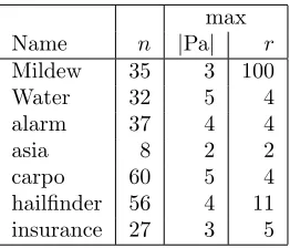
Name n |Pa| r

Mildew 35 3 100

Water 32 5 4

alarm 37 4 4

asia 8 2 2

carpo 60 5 4

hailfinder 56 4 11

insurance 27 3 5

Table 1: The seven Bayesian networks used in this paper. n is the number of variables, max|Pa| is the size of the biggest parent set and maxr is the max-imum number of values associated with a variable in the network.

N =. . .

Name 102 ₁₀3 ₁₀4

Mildew 100 1000 10000

Water 100 990 9368

alarm 94 805 5970

asia 16 30 52

carpo 100 995 9662

hailfinder 100 1000 10000

insurance 99 982 8918

Table 2: Number of distinct joint instantiations sam-pled from each ‘true’ BN whereN is the total number of joint instantiations.

2

Bayesian networks and datasets

Since the goal of this paper is to evaluate a particular approach to BN learning, all datasets are the result of sampling from a known ‘true’ BN. Seven BNs were used: their names and key characteristics are given in Table 1. Each BN only involves discrete variables. All BNs were obtained in Bayesian Interchange (.bif) format from the Bayesian Network Repository (http: //compbio.cs.huji.ac.il/Repository/). Each was then then converted into a Python class instance and ‘pickled’ (i.e. saved to disk).

Datasets of sizes 100, 1,000 and 10,000 were then gen-erated by forward sampling from each BN. Note that each dataset is complete: there are no missing values. Each dataset was stored as a single table in an SQLite database. Each such table had two columns: a string representation of each distinct joint instantiation sam-pled and a count of how often that joint instantia-tion had been sampled. For big BNs most or all of these counts will be one. Table 2 states the number of distinct joint instantiations for each dataset. Each SQLite database was wrapped inside a Python class instance which was then pickled.

3

Computing and filtering family

scores

The primary goal of this paper is to evaluate MaxWalkSat as an algorithm to search for BNs of high marginal likelihood for a given dataset. As is well known, if Dirichlet priors are used for the parameters of a BN and the data are complete then the marginal likelihood for a BN structureGfor dataDis given by the equations in (1) and (2) [3].

P(G|D) =L(G) =

n

Y

i=1

Scorei(G) (1)

where

Scorei(G) = qi

Y

j=1

Γ(αij) Γ(nij+αij)

ri

Y

k=1

Γ(nijk+αijk)

Γ(αijk) (2)

Equation (2) defines what will be called afamily score

since it is determined by a child variable and its par-ents. In (2), qi is the number of joint instantiations of those parents that Xi has in the graphG;j is thus an index over these instantiations. ri is the number of values Xi has and thus k is an index over these values. nijk is the count of how often Xi takes its

kth value when its parents are in their jth instanti-ation. αijk is the corresponding Dirichlet parameter. Finally, nij =Pri

k=1nijk and αij =

Pri

k=1αijk. Since Scorei(G) only depends on Pai, the parents it has in

graph G, Scorei(G) can be written as Scorei(Pai).

Throughout this paper the values of αijk have been chosen so thatL(G) becomes theBDeu metricfor scor-ing BNs. This is done by choosscor-ing a prior precision

valueαand settingαijk=α/(riqi). In this paper the prior precision was always set to α = 1. The BDeu score is a special case of a BDe score; BDe scores have the property that Markov equivalent BNs are guaran-teed to have the same score. Setting αijk = 1/(riqi) allows family scores to be defined by (3).

Scorei(Pai) = qi

Y

j=1 Γ(1

qi)

Γ(nij+ 1

qi)

ri

Y

k=1

Γ(nijk+ 1

riqi)

Γ( 1

riqi)

(3)

Now, let Xbe any subset of the variables and define, for fixed data, the functionH, as in (4).

H(X) =

qX

Y

ℓ=1

Γ(nℓ+ 1

q_X)

Γ( 1

q_X)

(4)

whereqX is the number of joint instantiations of

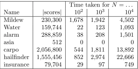
Time taken forN =. . .

Name |scores| 102 ₁₀3 ₁₀4

Mildew 230,300 1,678 1,942 4,502

Water 159,744 22 123 1,093

alarm 288,859 38 208 1,501

asia 512 0 0 0

carpo 2,056,800 544 1,811 13,892

hailfinder 1,555,456 852 2,974 22,666

insurance 79,704 29 97 749

Table 3: Computing all family scores with at most 3 parents. Times are in seconds rounded (asia did take a small positive amount of time!)

occurred in the data. Let Paibe the parents ofXiand

set Fai={Xi}∪Pai(thefamily forXi), then it is easy

to see that (3) can be rewritten as (5)

Scorei(Pai) =

H(Fai) H(Pai)

(5)

so that

log Scorei(Pai) = logH(Fai)−logH(Pai) (6)

In the approach followed in this paper the first stage of BN learning is to compute log family scores log Scorei(G) for all families up to some limit on the

number of parents. Here this limit was set to 3 parents. Note that 4 of the 7 true BNs have variables with more than 3 parents so that this restriction renders these 4 unlearnable. Equation (6) permits a small efficiency increase: logH(Fai(X)) is computed for all subsets of

variables from size 0 to size 4. Family scores can then be computed using (6). (All scores will be log scores from now on.)

The number of family scores computed and the time taken is listed for each dataset in Table 3. These computations were performed using Python equipped

with the Psyco (http://psyco.sourceforge.net/)

JIT compiler. Re-implementing in, say, C would no doubt be faster, but optimising this part of the pro-cess is not the focus of this paper.

Once family scores are computed the next step is to encode them as weighted clauses, but, with the excep-tion of asia, there are too many scores for all to be used. However, since the goal is to find high likelihood BNs the vast majority of these family scores can be thrown away. Let Paiand Pa′ibe two potential parent

sets for variableXi. If (1) Pai ⊂Pa′i and (2) Pai has

a higher score than Pa′

i then Pa′i can be ruled out as

a potential parent set for Xi in a maximal likelihood graph. Any graph which has Pa′

i as the parents for Xi can have its score increased by replacing Pa′

i by

Pai; the key point is that such a replacement cannot

N=. . .

102 ₁₀3 ₁₀4

Dat max n max n max n

Mi 977 3,515 17 163 47 465

Wa 44 482 44 573 49 961

al 75 907 184 1,928 473 6,473

as 10 41 24 107 31 161

ca 350 5,068 352 3,827 2,089 16,391

ha 22 244 77 761 435 3,768

in 28 279 95 774 496 3,652

Table 4: Results of filtering potential parents for vari-ables. ‘True’ BN names have been abbreviated. nis the total number of candidate parent sets for all vari-ables. max is the number of candidate parents for that variable which has the most candidate parents.

introduce a directed cycle since one or more arrows are being removed. Filtering family scores in this way causes a significant reduction in the potential parent sets for any variable as shown by Table 4.

4

Encoding BN learning using hard

and soft clauses

The goal of finding a maximum (marginal) likelihood BN with complete data is equivalent to choosing then

best parent sets (one for each variable) subject to the condition that no directed cycle is formed: a problem of combinatorial optimisation. Here this problem is encoded with weighted clauses.

A weighted CNF problem requires specifying (i) propo-sitional atoms (ii) clauses and (iii) weights for clauses. To represent graph structure two options have been considered. Using an adjacency matrix approach for each of the n(n−1) distinct ordered pairs of vertices there is an atom asserting the existence of an arc be-tween the two vertices. Alternatively one can create one atom for each possible family (child plus parents). This latter approach has performed better in the ex-periments done so far, presumably because flipping the truth values of such atoms permits bigger search moves. With this approach when encoding the prob-lem of learning from the carpo-generated dataset with 10,000 datapoints there are 16,391 such atoms (see Ta-ble 4). If such an atom is set to TRUE, this represents that the specified variable has the specified parents. For each variable there is a single clause stating that it must have a (possibly empty) parent set:

_

candidate parent set t

Xi has parent sett (7)

To rule out choices of parent sets producing a cycle two options have been considered. In the first ‘Ancestor’ encoding, there is an atom an(Xi, Xj) stating thatXi

is an ancestor ofXj in the graph for each of then(n−

1) distinct ordered pairs of vertices. For each of the

n(n−1)(n−2) distinct ordered triples (Xi, Xj, Xk) there is a transitivity clause:

an(Xi, Xj)∧an(Xj, Xk)→an(Xi, Xk) (8)

To express acyclicity there are n(n−1)/2 clauses of the form:

¬an(Xi, Xj)∨ ¬an(Xj, Xi) (9)

An alternative ‘Total order’ approach is to encode a total order of vertices. In a total order exactly one of Xi < Xj and Xj < Xi is true for each distinct

Xi and Xj. So for each of the n(n−1)/2 distinct unordered pairs{Xi, Xj}there is an atom ord(Xi, Xj) asserting thatXiandXj are lexicographically ordered in the total order. To ensure that an assignment of truth values to these atoms defines a total order it is enough to rule out 3-cycles such asXi< Xj,Xj < Xk,

Xk< Xi. This is because if a fully connected digraph with no 2-cycles (a tournament) has a cycle then it has a 3-cycle. There is a simple inductive proof of this result which is omitted here. There aren(n−1)(n−2) hard clauses ruling out 3-cycles of the form:

¬ord(Xi, Xj)∨ ¬ord(Xj, Xk)∨ord(Xi, Xk) ord(Xi, Xj)∨ord(Xj, Xk)∨ ¬ord(Xi, Xk)

Using either the ‘Ancestor’ or ‘Total Order’ encoding there are hard clauses declaring that a (non-empty) choice of parents for a variable determines the truth value of certain atoms. For example, using the ‘An-cestor’ approach:

Xj has parent set{Xi, Xk} → an(Xi, Xj)

Xj has parent set{Xi, Xk} → an(Xk, Xj)

or with the ‘Total Order’ approach:

Xj has parent set{Xi, Xk} → ord(Xi, Xj)

Xj has parent set{Xi, Xk} → ¬ord(Xj, Xk)

Note that since the log BDeu score is a log-likelihood it is a negative number, as are all the family scores. The goal is to find an admissible choice of families with small negative numbers. Another way of looking at this is to say that choosing any particular set of

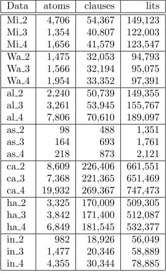
Data atoms clauses lits

Mi 2 4,706 54,367 149,123

Mi 3 1,354 40,807 122,003

Mi 4 1,656 41,579 123,547

Wa 2 1,475 32,053 94,793

Wa 3 1,566 32,194 95,075

Wa 4 1,954 33,352 97,391

al 2 2,240 50,739 149,355

al 3 3,261 53,945 155,767

al 4 7,806 70,610 189,097

as 2 98 488 1,351

as 3 164 693 1,761

as 4 218 873 2,121

ca 2 8,609 226,406 661,551

ca 3 7,368 221,365 651,469

ca 4 19,932 269,367 747,473

ha 2 3,325 170,009 509,305

ha 3 3,842 171,400 512,087

ha 4 6,849 181,545 532,377

in 2 982 18,926 56,049

in 3 1,477 20,346 58,889

in 4 4,355 30,344 78,885

Table 5: Data on the weighted CNF provided as input to MaxWalkSat using the ‘Ancestor’ encoding and a cycle atom. Datasets have been abbreviated, so that e.g. in 4 is the data set of 104_{datapoints sampled from}

insurance.

parents for a variable incurs a cost which is -1 times the relevant family score. Each such cost can then be encoded by a weighted clause of the following type:

−log Scorei(Pai) :¬(Xi has parent set Pai) (10)

The−log Scorei(Pai) costs were rounded to integers.

A final option is not to rule out cycles directly, but to create a cycle atom asserting the existence of a cy-cle. Cycles can then be ruled out entirely with the hard clause¬cycle atom or merely discouraged with a soft version. If the latter option is taken then cyclic digraphs have to be filtered out after the search is over.

The numbers of atoms, clauses and literals for an en-coding of each learning problem using a cycle atom and the ‘Ancestor’ encoding is given in Table 5. With-out a cycle atom there is one fewer atom and clause and also a reduction in the number of literals. With the ‘Total Order’ approach there is a small reduction in atoms and the number of clauses and lits is roughly halved. (A literal is an atom or its negation, the num-ber of literals in Table 5 is the sum of all literals in all clauses.)

the ‘Ancestor’ encoding as shown in Fig 1. This is a run using the encoded form of the hailfinder-generated set of 10,000 datapoints. This is a runwithout using the cycle atom so the numbers of atoms, clauses and literals are reduced a little from those given in Table 5. The goal was to find a BN with BDeu score at least as high as that of the ‘true’ BN’s score of -503,040 (i.e. cost of 503,400). This was achieved in just under 13 million flips taking 75 seconds.

A key point is that the number of unsatisfied clauses in the lowest cost assignment in each try is 56, the num-ber of variables in hailfinder. These unsatisfied clauses are 56 weighted single-literal clauses of the form (10) corresponding to a choice of parents for each variable which does not produce a cycle. In all runs on all datasets, the unsatisfied clauses in low cost assign-ments arealways of this form. Choices of parents that do cause a cycle will break at least one hard clause thus incurring a sufficiently large cost that MaxWalk-Sat will never return them as a lowest cost assignment. Note that although only one choice of parents is pos-sible for any variable there is no need to encode this (hard) constraint. Choosing e.g. two parent sets will always incur a higher cost then either or the two alone so the search avoids such assignments. MaxWalkSat ‘wants’ to avoid choosing any parents but is compelled to do so by hard constraints of the form (7).

5

Results

5.1 Learning a single BN

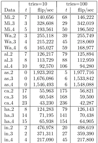
In this section, results using MaxWalkSat to search for a high BDeu-scoring BN are given. The scores from these searches are given in Table 6 and some timings are given in Table 7. Note that the times reported in Table 7 are for one of the slowest approaches: ‘Ances-tor’ encoding, 50% noise (random flips). An example of such a ‘slow’ run was shown in Fig 1 where only 171,206 flips/sec were achieved. In contrast, using the ‘Total Order’ encoding with 10% noise on the same data a rate of 1,092,243 flips/secs is achievable.

One problem with evaluating a search for a high scor-ing BN is that the optimal BN and its score is unknown (although presumably it could be computed for the small asia learning problem). However, by choosing to evaluate on synthetic data there is at least the ‘true’ BN which can be scored. It is also possible to con-struct a high-scoring BN which meets the restriction of having at most 3 parents. Starting with the true BN replace each true parent set with the highest-scoring pre-scored parent set which is a subset of the true par-ent set. With the exception of carpo this produces a BN with a higher score than the true BN. The score

tries=10 tries=100

Data t flip/sec t flip/sec

Mi 2 7 140,656 68 146,222

Mi 3 3 328,608 29 342,019

Mi 4 5 193,561 50 196,502

Wa 2 3 255,118 39 255,749

Wa 3 4 215,222 45 218,069

Wa 4 6 165,027 59 168,977

al 2 7 126,217 79 125,894

al 3 8 113,729 88 112,959

al 4 10 92,570 106 94,280

as 2 0 1,923,202 5 1,977,716

as 3 0 1,676,086 6 1,533,842

as 4 0 1,546,493 6 1,548,088

ca 2 17 55,963 175 56,821

ca 3 16 60,548 168 59,500

ca 4 23 43,230 236 42,287

ha 2 8 124,283 79 126,143

ha 3 14 71,195 141 70,438

ha 4 15 65,938 154 64,905

in 2 2 476,978 20 498,619

in 3 2 371,311 27 359,390

in 4 4 217,090 45 217,800

Table 7: Timings corresponding to ‘Ancestor’ encod-ing runs with a ‘cycle atom’ and noise at 50%. tis the total time taken in seconds (rounded). Flip/sec is the frequency of literal flipping performed by MaxWalk-Sat.

of the BN thus constructed is given in the ‘Target’ column of Table 6.

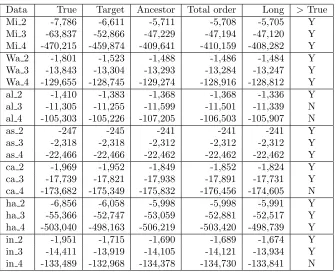
Table 6 contains only the most interesting of many experimental runs conducted. The results show that for small datasets (* 2, corresponding to 102 _{= 100),} MaxWalkSat easily finds BNs exceeding both the True and ‘Target’ BN score. This reflects the relatively smooth nature of the likelihood surface. For bigger datasets, were the landscape is much more jagged, the picture is more mixed. For 103 _{size datasets the True} BN score is beaten by the ‘Long’ run in all cases, except for alarm. For 104_{, the ‘Long’ run fails to} beat carpo and insurance also. Comparing ‘Ances-tor’ to ‘Total Order’ results show that the latter is the

more successful encoding. Experiments unreported

here have indicated that the ‘Total Order’ encoding works better with low noise (random flip) values and a prevention of random breaking of hard clauses. Com-bining these with an increased search on each try leads to the superior results in the ‘Long’ column of Table 6. Note that even the longest ‘Long’ run, ca 4, only took 32 minutes (with 510,397 flips/sec); most where much faster.

newmaxwalksat version 20 (Huge) seed = 99955222

cutoff = 10000000 tries = 100 numsol = 1

targetcost = 503040

heuristic = best, noise 50 / 100, init initfile allocating memory...

clauses contain explicit costs

numatom = 6848, numclause = 181544, numliterals = 529296 wff read in

average average mean

lowest worst number when over flips

cost clause #unsat #flips model success all until this try this try this try this try found rate tries assign

506076 16968 56 10000000 * 0 * *

501973 23318 56 2913803 2913803 50 12913803 12913803.0

total elapsed seconds = 75.428415 average flips per second = 171206 number of solutions found = 1

mean flips until assign = 12913803.000000 mean seconds until assign = 75.428415 mean restarts until assign = 2.000000 ASSIGNMENT ACHIEVING TARGET 503040 FOUND

Figure 1: A successful search (using the ‘Ancestor’ encoding) for a BN exceeding the BDeu score for the hailfinder BN using data of 10,000 data points sampled from that BN.

Data True Target Ancestor Total order Long >True

Mi 2 -7,786 -6,611 -5,711 -5,708 -5,705 Y

Mi 3 -63,837 -52,866 -47,229 -47,194 -47,120 Y

Mi 4 -470,215 -459,874 -409,641 -410,159 -408,282 Y

Wa 2 -1,801 -1,523 -1,488 -1,486 -1,484 Y

Wa 3 -13,843 -13,304 -13,293 -13,284 -13,247 Y

Wa 4 -129,655 -128,745 -129,274 -128,916 -128,812 Y

al 2 -1,410 -1,383 -1,368 -1,368 -1,336 Y

al 3 -11,305 -11,255 -11,599 -11,501 -11,339 N

al 4 -105,303 -105,226 -107,205 -106,503 -105,907 N

as 2 -247 -245 -241 -241 -241 Y

as 3 -2,318 -2,318 -2,312 -2,312 -2,312 Y

as 4 -22,466 -22,466 -22,462 -22,462 -22,462 Y

ca 2 -1,969 -1,952 -1,849 -1,852 -1,824 Y

ca 3 -17,739 -17,821 -17,938 -17,891 -17,731 Y

ca 4 -173,682 -175,349 -175,832 -176,456 -174,605 N

ha 2 -6,856 -6,058 -5,998 -5,998 -5,991 Y

ha 3 -55,366 -52,747 -53,059 -52,881 -52,517 Y

ha 4 -503,040 -498,163 -506,219 -503,420 -498,739 Y

in 2 -1,951 -1,715 -1,690 -1,689 -1,674 Y

in 3 -14,411 -13,919 -14,105 -14,121 -13,934 Y

in 4 -133,489 -132,968 -134,378 -134,730 -133,841 N

which is astronomically more probable (assuming a uniform prior) than the ‘true’ one. For example, with Mi 2 and the Ancestor encoding, the returned BN is

e(−470,215+409,641) _{= e}60,574 _{more probable than the} true one!

A rough comparison with Castelo and Koˇcka’s RCARNR and RCARR algorithms [1] is possible for the al 2 and al 4 datasets. As here, datasets of size 1,000 and 10,000 were sampled from the Alarm BN and best scores of around -11,115 and -108,437 respec-tively were reported. This beats (resp. does not beat) our best score for Alarm, but since the actual sampled datasets are different not too much should be read into this comparison.

Some initial experiments adding prior knowledge to the ‘Ancestor’ encoding proved interesting. Adding in information specifyingall known pairs of independent variables (by banning the relevant ancestor relations) had very little effect on the scores achieved. On the other hand, setting just a small number of known an-cestor relations improved scores considerably. This is presumably due to the search having a bias towards sparser (less constrained) BNs.

5.2 Bayesian model averaging by search

Markov chain Monte Carlo (MCMC) approaches are popular for Bayesian model averaging (BMA) for Bayesian networks. The idea is to construct a Markov chain whose stationary distribution is the true poste-rior over BNs. By running the chain for a ‘sufficient’ number of iterations (and throwing away an initial burn-in) the hope is that the sample thus produced supplies a reasonable approximation to the true distri-bution.

Success depends on a realisation of the chain wander-ing into areas of high probability and visitwander-ing different BNs with a relative frequency close to the BNs’ pos-terior probabilities. A search-based approach offers a much more direct method of BMA. The key idea is to explicitly search for areas of high probability. If, as is the case here, the probability of any visited BN can be computed at least up to a normalising con-stant then this value is recorded. An estimate of the posterior distribution is then found by simply assign-ing zero probability to any BN not encountered in the search and performing the obvious renormalisation on BN scores. An early paper proposing search for BMA is [4].

Here a crude search-based approach using MaxWalk-Sat and the ‘Ancestor’ encoding has been tried out. MaxWalkSat is run as normal and for every assign-ment where no hard clause is broken a record of the

n parent sets given by that assignment together with

0 0.1 0.2 0.3 0.4 0.5 0.6 0.7 0.8 0.9 1

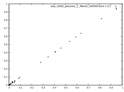
0 0.1 0.2 0.3 0.4 0.5 0.6 0.7 0.8 0.9 1 ’asia_10000_pascores_3._filtered_1000000.bma’ u 2:3

Figure 2: Comparing estimated posterior probabilities from two different BMA runs using MaxWalkSAT us-ing asia 10,000 data

the cost of the assignment is sent to standard output. Piping this through UNIX’ssort --uniqueis enough to produce a list of distinct (encoded) BNs sorted by score.

The distribution thus created can be used to estimate true posterior quantities. In experiments conducted so far only the posterior probabilities of parent sets have been estimated. By comparing estimates pro-duced from two runs, some measure of success can be produced. Here each run used the ‘Ancestor’ encoding and came from 120 restarts of MaxWalkSat each using 100,000 flips. Only the 1,000,000 highest scoring BNs from each run were kept.

For the datasets considered here only asia (all sizes) and Water with 100 datapoints afforded successful BMA. Plots comparing estimated posterior probabil-ities for parent sets for these two cases are given in Figs 2 and 3. In all other cases such plots show big differences in estimated probabilities for most cases where the estimates differ significantly from zero. Fig 4 shows a typical excerpt of such a failure using the alarm 100 data.

0 0.1 0.2 0.3 0.4 0.5 0.6 0.7 0.8 0.9 1

0 0.1 0.2 0.3 0.4 0.5 0.6 0.7 0.8 0.9 1 ’Water_100_pascores_3._filtered_1000000.bma’ u 2:3

x

Figure 3: Comparing estimated posterior probabilities from two different BMA runs using MaxWalkSAT us-ing Water 100 data

1622 9.89412087285e-35 5.71801239082e-28 1793 0.0013149823888 0.465138403992 1792 1.51462961172e-20 5.38296345824e-18 1791 5.89129801134e-14 2.10283310245e-06 1398 0.924408916903 0.00117720289971 1797 1.46223426395e-06 1.77652663003e-11

Figure 4: Estimates of posterior probability of parent sets from two different BMA runs for AlarmN = 100 dataset. The first column is the integer identifier for the parent set used by MaxWalkSat.

models or needs to move in a more regular space, such as the space of variable orderings [2].

6

Conclusions

The results given here should be seen as a preliminary exploration of the worth of weighted MAX-SAT en-codings of BN learning and MaxWalkSat as a method for solving such encoded problems. In particular, fu-ture work needs to consider alternative encodings and greater incorporation of prior knowledge on structures. Exponential-family structure priors whose features can

C 176696 3954 4048 4197 4262 ... 17333 ... C 176714 3954 4048 4197 4262 ... 17332 ...

Figure 5: Top two BNs from a BMA run using the carpoN = 10,000 data. First number is the (rounded, negated) BDeu score. First one is 65 million times more probable (assuming a uniform prior) than second even though they differ in only one parent set (17333 vs. 17332).

be easily encoded are an obvious choice; they can be encoded by weighted clauses, just as the family scores are. This paper has focused on BN learning as a pure BDeu score optimisation problem. Further work will consider the value of the learned BNs according to other metrics and provide a comparison of this learn-ing approach with existlearn-ing BN learnlearn-ing systems.

How to reproduce these results Please go to:

http://www.cs.york.ac.uk/∼_{jc/research/uai08/}

Acknowledgements

Thanks to those responsible for hosting the Bayesian Network Repository and to Henry Kautz for making MaxWalkSat available. Thanks also to 3 anonymous reviewers.

References

[1] Robert Castelo and Tom´aˇs Koˇcka. On inclusion-driven learning of Bayesian networks. Journal of Machine Learning Research, 4:527–574, 2003.

[2] Nir Friedman and Daphne Koller. Being Bayesian about network structure: A Bayesian approach to structure discovery in Bayesian networks.Machine Learning, 50:95–126, 2003.

[3] David Heckerman, Dan Geiger, and David M. Chickering. Learning Bayesian networks: The com-bination of knowledge and statistical data. Ma-chine Learning, 20(3):197–243, 1995.

[4] David Madigan and Adrian E. Raftery. Model se-lection and accounting for model uncertainty in graphical models using Occam’s window. Journal of the American Statistical Association, 89:1535– 1546, 1994.

[5] Hoifung Poon and Pedro Domingos. Sound and efficient inference with probabilistic and determin-istic dependencies. InProc. AAAI-06, pages 458– 463, 2006.

[6] Tian Sang, Paul Beame, and Henry Kautz. Solving Bayesian inference by weighted model counting. In

Proc. AAAI-05, Pittsburgh, 2005.

[7] Tian Sang, Paul Beame, and Henry Kautz. A dy-namic approach to MPE and weighted MAX-SAT. InProc. IJCAI-07, Hyderabad, 2007.

[8] Bart Selman, Henry Kautz, and Bram Cohen. Lo-cal search strategies for satisfiability testing. In David S. Johnson and Michael A. Trick, editors,