Central limit results without independence

by

Robert Joseph Adler, B.Sc.(Hons) Sydney

A thesis submitted for the degree of Master of Science at

The Australian National University, Canberra.

The author wishes to acknowledge the assistance given to him by his supervisor, Dr. C.C. Heyde, who was always avail­ able for comment and discussion, even when we were separated by some thousands of miles. He also thanks Miss Norma Chin, whose excellent typing has turned a somewhat messy manuscript

into a readable and presentable form. Finally, thanks are due to the author's wife, Joan, and his daughter, Arielle, both of whom have, in their own way, made this thesis

CENTRAL LIMIT RESULTS WITHOUT INDEPENDENCE

CONTENTS

INTRODUCTION 1

CHAPTER I - MARTINGALE CENTRAL LIMIT RESULTS 3

1.1 Preliminaries 3

1.2 Brown’s Theorem 7

1.3 Scott's Theorem 8

1.4 Drogin's Theorem 12

1.5 AnConoralioation of Drogin's Theorem 14

CHAPTER II - RELAXING THE LINDEBERG CONDITION FOR MARTINGALES 19

2.1 Zolotarev's Theorem 20

2.2 Two Central Limit Theorems 24

2.3 On an Invariance Principle 34

CHAPTER III - QUESTIONS OF NECESSITY 38

3.1 Necessary and Sufficient Conditions when the

Summands are Independent 39

3.2 Some Necessary Conditions for Martingales 40 3.3 A Necessary and Sufficient Form of Drogin's Theorem 45

This thesis is primarily concerned with central limit results for martingales, and the role Lindeberg-type conditions play in them. Two types of results are dealt with, simple one-dimensional central limit theorems and more complex invariance principles for the central limit theorem. Some of our results are more general or slightly different versions of known results, while others, within the context of

martingale theory, are completely new.

We begin in Chapter I by introducing the notation and the problems we shall consider. Also, as much of the earlier work relevant to our study has not yet been published, we spend some time describing and discussing it. The last part of the chapter derives two new invariance principles, the first of which is a subsequence version of a theorem of Scott [16] , while the second takes an invariance principle relating to a random subsequence of a martingale process (Drogin [8]) and derives a new version relating to a similar non-random subsequence.

In Chapter II we take the Lindeberg condition, which appears in some form in all the theorems of Chapter I, and, while still retaining a central limit theorem, weaken it in a manner analogous to Zolotarev's weakening of the Lindeberg condition in the classical Lindeberg-Feller

theorem for sums of independent random variables [19]. The aim here is to remove from the martingale differences the standard condition that they be uniformly asymptotically negligible (u.a.n.). In this chapter we also show that once the u.a.n. condition is lifted, simple

Chapter III considers the problem of necessity in more detail. Invariance principles of the type we consider contain a considerable amount of information, much of which can be conveniently retrieved using mappings of the random functions involved, together with

Theorem 5.1 of Billingsley [3]. Using this technique we are able to obtain the necessity and sufficiency of both the u.a.n. and Lindeberg conditions in a functional analogue of the classical Lindeberg-Feller theorem, as well as deriving some general, necessary conditions for invariance principles involving martingales and other stochastic

processes. The main result of this chapter is an invariance principle for martingales in which the convergence in the mean of order one of a Lindeberg sum to zero is sufficient for weak convergence, while

Chapter I

Martingale Central Limit Results

1.1 Preliminaries

There has existed for some time a large body of literature con­ cerned with central limit theorems for sums of independent random variables. Recently a considerable amount of work has been done extending these results to cases when the summands are no longer independent. In this chapter, which serves as an introduction to the terminology, notation, and concepts of the later chapters, we shall review some of this work, as well as establishing two new results.

Various forms of dependence among summands have been used in generalising independence results, among the more important being con­ ditions of stationarity, m-dependence, mixing, and martingale

dependence. Serfling [17] has obtained, under a certain set of moment conditions, combined with a Lindeberg-type condition, central limit theorems for sequences of random variables satisfying each of these types of dependence, and his paper serves as a good introduction to the various classes of dependence currently in the literature. In what follows however, we shall be concerned exclusively with martingale dependence. There are two main reasons for this, which we shall state after having defined exactly what we mean by a martingale.

Let {ft,F,P} be a measure space: Ü is a set, F is a a-field of subsets of $7, and P is a probability measure defined on F. Let

information contained in the past history of the process. Then if the following three conditions hold, the sequence of random variables (Sn , n > 1} is said to be a martingale relative to {F , n > 1}.

(i) S is measurable with respect to F ,

n r n *

(ii) EIS I < », ! n 1 *

(iii) If m < n, then E(S |F ) = S a.s.

“ n 1 m m

We shall refer to this sequence of random variables as the martingale {Sn ,Fn> n > 1} defined on the probability space {fi,F,P}.

The simplicity and ensuing generality of martingales is the first reason to study this form of dependence. The second and more

important reason is the rather useful fact that it is possible to obtain from any integrable stochastic process a closely related

martingale by appropriate subtraction of conditional expectations. If

n n

Z.} is any integrable process then { £ [Z. - E(Z.|z. , , ...)]}

I J j=l J J J-i

{

a martingale relative to the sequence of o-fields generated by , j < n. Often the conditional expectations of a process, given the past, have a simple form, and thus central limit results are easy to establish if corresponding results are already known to hold for martingales. Furthermore Scott [16] has developed a representation, due originally to Gordin [20], which shows that the increments of a stationary process can, under mild conditions, be represented as the increments of a

stationary martingale plus extra terms which telescope under summation and disappear under the usual normings. Such results indicate the importance of martingales in the much wider field of dependent random variables.

sufficient condition for the asymptotic normality of the sum, under an appropriate uniformity condition on the summands.

The Lindeberg-Feller Theorem

Let {X., j > 1} be a sequence of independent random variables with n

EX. = 0, EX? < 00 Vj, and with partial sums S = 2 X.. Let

J J n j=i J

s2 = E(S2) and write F. for the distribution function of X.. Then if

n n j j

sup E(Xf)/s- 0 as n -> °°, the following (Lindeberg) condition is

j-n 3 n

v

v

necessary and sufficient for s 1 S ■> N(0,1) as n ■+ », where denotes convergence in distribution,

n j*

s” 2 2 X2 dF.(x/s ) 0 as n -* Ve > 0 .

n . it j (ii)**v n *

j=l J |x|>e

It seems natural to study a martingale analogue of the above theorem, and particularly the role that some analogue of the Lindeberg condition has to play for a martingale sequence. Central limit

theorems and invariance principles for martingales, using such con­ ditions, have already been found by Brown [4], [5], Brown and Eagleson

[6], Drogin [8], and Scott [16J , all of whom used quite different techniques, and, quite often, different sequences and norming factors. Underlying all of these results however is some form of Lindeberg con­ dition for martingales, which we now describe in its simplest form.

Consider the martingale defined above. Then we can define a sequence of martingale differences as follows:

(i) X = S = 0 a.s.

o o

(ii) X = S - S - , n > 1. n n n - 1

We shall suppose that EX2 < 00 for each n. If we now write s2 = E(S^), n > 1, we can say that the martingale satisfies the Lindeberg

j = l

E(x! I(lxj

> e s

n } ■ > 0 1 . 1. 1

a s n Ve > 0 , w h e r e 1(A) i s t h e i n d i c a t o r f u n c t i o n o f t h e s e t A, P

and d e n o t e s c o n v e r g e n c e i n p r o b a b i l i t y . 1 . 1 . 1 o f c o u r s e r e d u c e s t o

t h e c l a s s i c a l f o r m o f L i n d e b e r g c o n d i t i o n i n t h e c a s e o f i n d e p e n d e n c e .

Two m ai n t h eme s r u n t h r o u g h t h i s t h e s i s . F i r s t l y , i s i t p o s s i b l e

t o r e l a x t h e L i n d e b e r g c o n d i t i o n i n t h e r e s u l t s m e n t i o n e d a b o v e t o

o b t a i n a w e a k e r s e t o f c o n d i t i o n s f o r t h e m a r t i n g a l e t h a t i s s t i l l

s u f f i c i e n t f o r a c e n t r a l l i m i t r e s u l t ? The m o t i v a t i o n b e h i n d t h i s i s

d e s c r i b e d i n C h a p t e r I I . S e c o n d l y , w i t h t h e e x c e p t i o n o f Brown [ 5 ] ,

a l l o f t h e a b o v e p a p e r s h a v e c o n s i d e r e d o n l y t h e s u f f i c i e n c y o f t h e i r

c o n d i t i o n s f o r o b t a i n i n g f u n c t i o n a l c e n t r a l l i m i t t h e o r e m s ( i n v a r i a n c e

p r i n c i p l e s ) , and t h e on e e x c e p t i o n c o n t a i n s a r a t h e r r e s t r i c t e d r e s u l t .

I s i t p o s s i b l e t h e n , w i t h i n t h e f r a m e w o r k o f a n i n v a r i a n c e p r i n c i p l e ,

t o o b t a i n g e n e r a l n e c e s s a r y and s u f f i c i e n t c o n d i t i o n s f o r t h e

c o n v e r g e n c e o f a m a r t i n g a l e s e q u e n c e ?

I n C h a p t e r I I we s h a l l show t h a t t h e f i r s t o f t h e s e p r o b l e m s c a n

b e s o l v e d u s i n g a s i m i l a r a p p r o a c h t o t h a t t a k e n by Z o l o t a r e v [19J i n

s o l v i n g t h e same p r o b l e m i n t h e i n d e p e n d e n c e c a s e . C h a p t e r I I I

p r o v i d e s a p a r t i a l a n s w e r t o t h e s e c o n d p r o b l e m u s i n g a v a r i e t y o f

t e c h n i q u e s .

B e f o r e we a c t u a l l y t a c k l e t h e s e p r o b l e m s f u l l y i t i s w o r t h w h i l e t o

s p e n d some t i m e r e v i e w i n g , i n r e a s o n a b l e d e t a i l , r e c e n t wo rk i n

m a r t i n g a l e c e n t r a l l i m i t t h e o r e m s . B e c a u s e much o f t h e wo rk we s h a l l

r e f e r t o h a s n o t y e t b e e n p u b l i s h e d , i t w i l l b e n e c e s s a r y t o q u o t e some

t h e o r e m s i n f u l l , an d t o g i v e s k e t c h e s o f t h e i r p r o o f s .

The h i s t o r y o f m a r t i n g a l e c e n t r a l l i m i t t h e o r e m s a c t u a l l y d a t e s

invariance principle for stationary, ergodic martingales. The results

of immediate concern to us however, are those of Brown [3], Scott [16]

and Drogin [8], whose results are written out below as Theorems 1.1 to

1.3.

1.2 B r o w n ’s Theorem

Theorem 1.1, which we shall call Brown's Theorem for the remainder

of this thesis, was the first, chronologically, of the three results

following, and is perhaps also the simplest of them. Brown's result is

actually an invariance principle, in which he considers a random

function, £n , defined on the martingale, with realisations (sample

paths) in C = C[0,1], the space of continuous functions on [0,1], He

defines

= s ' 1 S,

n k

sk s t s 2 < s 2 n " Sk+1 + X.

(ts2 - s 2)

n k

k+1 (s2

k+1

3&

1. 2. 1

for 0 < t < 1, and s£ < ts^ < s£+ ^, k = 0,1,2, ..., n-1. Then is

a.e. continuous on [0,1] for all n, being composed of straight line

segments joining the points (sn 2s 2 ,sn LSk ) and (sn 2s£+ 1 >

snl

k = 0,1, ..., n-1. Furthermore, write W for a standard Wiener process

(Brownian Motion) in C, with the properties defined on page 61 of [3].

The existence of such a W is established in [3]. Then Brown's result

can be stated as follows.

Theorem 1.1

Retain the above notation. Then

V

£ -> W as n -* 00

n 1.2.2

n P

s“2 2 E(X?|F. .) + 1 as n -> « , 1.2.3

n - I J J-l J = 1 J J

n p

s 2 2 E(X2 I ( IX. > es ) IF. ,) + 0 as n + «>, Ve > 0 . 1.2.4 n . . j 3 ! ” n 1 i-l

J = 1 J

Like most other invariance principles of this type, Theorem 1.1 is

proven in two steps. Firstly, Brown shows that the finite dimensional

distributions of approach those of W, and then that the set of

measures associated with these finite dimensional distributions is

relatively compact (tight). Theorem 8.1 of Billingsley [3] then

guarantees the weak convergence of the random functions. The first

part of the proof is based on manipulation of characteristic functions,

following a technique developed by Billingsley [1], [2]. The same

technique is used in Chapter II of this thesis. The tightness proof

relies on an .upcrossing inequality for martingales derived by Doob [7].

As noted above, Brown's Theorem is perhaps the simplest we shall

consider. It is a result that involves the full martingale sequence

(some later results relate essentially only to subsequences of the

martingale) and the norming factor, s2 , is the intuitively obvious one.

Brown also provides a set of equivalent conditions to 1.2.3 and

1.2.4, but as these also arise in Scott’s Theorem we shall not state

them now. Another result of Brown’s, which contains a necessary as

well as sufficient condition for convergence of a subsequence of the

normed martingale is described in Chapter III.

1.3 Scott’s Theorem

Many of the random functions that we shall deal with are different

from in that they have sample paths in D[0,1] rather than C[0,1J.

Here D = D [0,1] is the space of real functions on [0,1] which are

to working in D rather than C. Firstly, since D contains C, the results in D have more scope and, as we shall see in Chapter III, necessity results are easier to obtain in D than in C. (It is of course imprecise to speak of "results in C or D" as we do here, since

convergence in distribution is always relative to a metric space. The

metric spaces we shall use are (D,p) and (C,p), where p is the sup-norm (uniform) metric. As we shall always be using the metric p with these function spaces, we shall continue to use this convenient expression.

The space (D,p) is used rather than the apparently more natural (D,d) because the limit distribution in all cases under consideration is con­

centrated in C. In these cases it is not hard to show that convergence

in (D,d) is equivalent to convergence in (D,p). The advantage of (D,p)

will become apparent whe n we move on to proving necessity results

using Billingsley’s continuous mapping theorem, to be described later.)

The function q^, defined below, has sample paths in D, and is the

function that Scott [16] works with.

n (t) = s" 1S, 1.3.1

n n k

for 0 < t < 1, s2 < ts2 < s 2 . , k = 0,1, ..., n.

k - n k+1 *

For this function the following result holds.

Theorem 1.2

Any one of the following five equivalent sets of conditions is

sufficient for

V

q ->■ W as n -* 00 .

n 1.3.2

n p

s 2 2 X 2 •* 1 as n 00

(A)

n . . ] J = 1 and

s 2 2 X 2 I ( X . > es ) + 0 as n ->

n . 1 J J n

3 = 1 J

1.3.3

CB)

5 2 2 E(X? F. .) 1

n - 1 J J - l

J = 1 J

as n > «

and

r

E

I

I

1.3.5

as Ve > 0 , 1.3.6

(C) and

s 2 2 X 2 ■+ 1 as n 00

n j-i J

s 2 sup X 2 -> 0 as n + “ ,

n . i *

J<n J

1.3.7

1.3.8

(D)

n P

s” 2 2 X 2 -> 1 as n “

n j-i J and

n P

s” z 2 X 2 U( |X. I / (es )) -* 0 as n Ve > 0 ,

n j=l 3 3 n

1.3.9

1.3.10

(E)

P

f 2 2 E (X ?

I

and

s“ 2 2 E(X2 U(|X |/(es )) |F ) l 0 as n+<=o, Ve > 0

l i = l J J J

1.3.11

1.3.12

where U is any continuous non-negative function of bounded variation on

[0,°°) for which U(0) = 0 and U(x) converges to a positive constant as

x °°.

One of the main points to note about this theorem is the set of

equivalent conditions it provides. This will be of significant value

later, when we attempt to show the necessity of a Lindeberg condition.

It is intuitively clear that conditions such as (B) above would be very

difficult to establish as necessary, whereas condition (C), which

resembles the conditions of Raikov (see [11], page 143), would seem

easier to derive from the convergence of to W. That this is in fact

the case will be shown in Chapter III.

Scott's proof of Theorem 1.2 is markedly different from that of

representation theorem given by Strassen, as Theorem 4.3 of [18]. Essentially what Scott does is to embed the martingale into a Brownian motion, and then show that appropriate sums of the stopping times that define the embedding approach any given value of the time parameter of a Wiener process. The a.s. (uniform) continuity of the Wiener process then ensures the convergence in probability of the finite dimensional distributions of nn to those of W as n °°. An appeal to Theorem 3 of Loynes [14], which proves that if the finite dimensional distributions

V

of nn approach those of W then nn W as n -* °°, completes the proof.

1.4 Drogin's Theorem

Although the results of Brown and Scott relate to different random functions they still have a great deal in common. Both relate to the full martingale sequence S , and to the "natural" norming factor s^. Drogin [8] has recently obtained some sufficient, and partly necessary, conditions for invariance principles involving random subsequences of the martingale, with a rather different method of norming.

n n

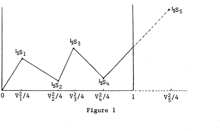
Let W2 = 2 X? and V 2 = 2 E(X?|F. ,). Define T =inf{m:V2 >n}. n j = l J n j = i J J"1 n m " Then Drogin forms the continuous random function 3 on [0,°°) by the

requirements that 8(0) = 0 , 8(V^) = Sm> and 8 is linear on [V^jV^^] . In the same way he forms y, using W^ instead of V^. Then he defines 8n and y^, both continuous functions on [0 ,1], defined at t by

8 (t) = 8(nt)/n2 and yR (t) = y(nt)/n. Thus 8R and yn have sample paths in C, being composed of straight line segments joining the points

(v£/n, Sk /n's) to (v£+1/n, S^j/n*5) and (W^/n,

Sjn'*)

Figure 1

For these functions, Drogin has proven the following result.

Theorem 1.3

Suppose EX2 < 00 Vj > 0, and V 2 -* 00 a.s. Then (A), (B) , and (C) are equivalent, and if they are true, so is (D).

(A)

_. n L

n 1 2 x 2 I(X? > ne) -* 0 as n Ve > 0 j = l 3 3

1.4.1

(B) and

sup

|v?

n~ 1 V 2 -> 1 as n -> 00 . in

1.4.2

1.4.3

(C)

\

3 W as n ■> n

n 1 V 2 -> 1 as n -* in

1.4.4

1.4.5

and

sup 13 (t) - y (t) I 0 as n ->• 00 0<t<l n n

y -> W as n -> 00 .

1 T t

1.4.6

where -> indicates convergence in the mean of order 1.

There are many aspects of this result that are of importance to us. Firstly, it does, to a degree, show the necessity of a Lindeberg-type

V

condition. However in order to derive 1.4.1 from 3 W it also n

requires 1.4.5 to hold, and this is a rather strong restriction. Although we have been unsuccessful in dealing with 3R , in Chapter III we shall show that if we redefine y^ slightly so that its sample paths

lie in D, the convergence of this new function to W is sufficient for 1.4.1, with convergence in mean replaced by convergence in probability.

The second point to note about Drogin's Theorem is the new method of norming the martingale it introduces, which is quite different from that used in the last two theorems. Finally, it is important to note that Theorem 1.3 relates only to a (random) subsequence of the

martingale, rather than the full sequence. As will become evident later, it is in many ways easier to show the necessity of a Lindeberg-type condition in this case.

Drogin's proof of Theorem 1.3 is quite different again from those of the previous theorems. It is based on the fact that, for large n, 3n and y^ both behave approximately like a fair coin random walk with small steps. As this type of proof will not be used in this thesis, it will not be described in detail.

As we have already noted, one of the major drawbacks of Drogin's Theorem is that it involves a random subsequence of the martingale. The following section removes this drawback by modifying the method of norming the martingale so that rather than using the conditional

1.5 Ao G one ralioatiott of Drogin's Theorem

Before progressing to the gonera-lioation of Drogin's Theorem, we

shall state without proof a lemma that generalises Scott's Theorem to

subsequences of the martingale. Its result is actually of some

interest in itself, as it can be easily shown that similar results hold

in the independence case, but we shall not examine its full import here.

Essentially what the lemma says is that if any martingale subsequence

satisfies subsequence versions of the conditions of Theorem 1.2, then

this subsequence, suitably normed, approaches normality. A correspond­

ing invariance principle also holds. The proof of the lemma follows

Scott's original proof of Theorem 1.2 in detail, the only changes being

in the upper limits of summations, and thus we shall not reproduce the

proof here.

ing the notation of Theorem 1.2, if any one of the following three

equivalent sets of conditions holds Lemma 1.1

Let { n . b e some subsequence of the positive integers.

Retain-l Retain-l — Retain-l

s~ 2 2 X? -> 1 as i -* 00 n. . 1 J

l j = l J

1.5.1

(A*) sand

n

P

> es ) -* 0 as i -* °°, Ve > 0

n. 1.5.2

i P

2 E(XJ|F ,) + 1 = 1 J J

as i -> oo 1.5.3

(B*) Sand

(C*) -sand

i p

s 12 2 X 2 -> 1 as i + n . . , j

l j = l J

s 2 sup X 2 -* 0 as i , n - . J

1 3<*± J

1.5.5

1.5.6

V

then n ->W. as i -> oo. n .

l

u<irG cc->»a

We are now in a position to state and prove our generalioation of

Theorem 1.3. Firstly, redefine T by T = inf{m:s2 > n}. Thus T is

n J n m - n

no longer a random variable. We form the random function L as n u

Cn (t) = S k/ n 2 for s 2 < tn < s 2+ 1 , k = 0,1, . . ., T -1, and t € [0,1] .

Then has sample paths in D, and the following result holds.

Theorem 1.4

and

1 11 L

- Z X 2 I (X2 > ne) + 0 , as n + » v e > o ,

n j=1 J J "

J = 1 J J

as n -> 00 ,

1.5.7

1.5.8

V

then C W as n -> °°. n

Before we prove T h e orem 1.4 we need to introduce a result of

B i l l i n g s l e y ’s (Theorem 5.1, [3]) which we shall refer to as his con­

tinuous mapping theorem. This result, stated below as Theorem 1.5,

guarantees the preservation of weak convergence under almost surely

continuous mappings. The corollary describes the same result in terms

of convergence in distribution.

Let {Xn } be a sequence of random elements on some metric space

(S,S), and let {Pn ) be their distributions. Denote the weak conver­

gence of these distributions to the distribution P of X by ^ P. Let

h be a measurable mapping of S into another metric space ( S ’,S’) and

measure P on (S,S) induces on (S',S') a unique probability measure Ph- *, defined by Ph"1(A) = P(h_1A) for A e 5'. Billingsley [3] has

established the following result.

Theorem 1.5

If P => P and P ( D J = 0, then P h"1 =► Ph"1.

n h * n

Corollary

For a random element X of S, h(X) is a random element of S'. Thus

V

V

if Xn -* X and P(X 6 Dh ) = 0, then h(X ) ■> h(X).

Proof of Theorem 1.4

We are now in a position to commence proving Theorem 1.4. To

V

prove it we introduce Scott's p , (1.3.1), show that p^ -> W and then

p n

that sup |pT (t) - £ (t) I -► 0 as n ■> °°. Theorem 4.1 of Billingsley

te [0,1] n p

[3] then guarantees Cn W as n -* 00.

Firstly we note that

1 < s| /n < n

1 + sup E(X?)/n j <T _n J

< 1 + e + sup E(X? I(X? > ne))/n j <T J 2

n Tn

< 1 + e + 1/n E 2 X? I(X? > ne) j = l J J

-> 1 + e as n 00 ,

and since e > 0 is arbitrary we have

s^ /n 1 as n -► 00 . n

Applying 1.5.9 to the conditions of the theorem, and noting that

1.5.9

11 L

s 2 2 X? I(X2 > £S2 ) -* 0 as n -*■ °° ,

in j=i 3 J in which implies

Tn i p

s“2 2 E (X2 I ( IX

J

1n j=i 3 J in 3 1

and

xn p

s”2 2 E(X?|F. ,) ■> 1 as n ■* 00 . in j = i J 3

But the last two conditions appear in Lemma 1.1. Thus we have that

V

nT -> W as n -* 00 . 1.5.10 in

Now note that

sup U-.Ct) -

nT

I

|s./sT

I

te[0,l] n j<Tn J n n

Consider the distribution of S,/s . Let Y = sup|w(t)|. From

F

n

t

Billingslay [^] (page 3 3 0 .) we have the distribution of Y.

P(Y<b) „ iL s iziil e- 2 ( 2 k + D 2/8b2 . TT i i ^rC i i.

k=l Given e > 0, choose b such that

e

P(Y > b ) < e .

Now, using Billingsley’s continuous mapping theorem, 1.5.10 implies that we can find an ni(e) large enough such that

P(sup

|s./sT I

e

jiTn J

Choose next an n2(e) so that

11 — s //n| < e/b Vn > n2 •

in b

Thus

P ( s u p I S / s | . | l - s / v/n I

j < T n J n

su p IS ( t ) - n ( t ) I 0

t € [ 0 , l ] n

and t h e p r o o f o f t h e t h e o r e m i s c o m p l e t e .

> £ ) < £ .

Chapter II

Relaxing the Lindeberg Condition for Martingales

Zolotarev [19] has proven what he calls a "Generalised Lindeberg-Feller Theorem" in which he shows that the uniform asymptotic

negligibility (u.a.n.) condition in the standard Lindeberg-Feller central limit theorem for sums of independent random variables can, under certain conditions, be dispensed with. The aim of this chapter is, by generalising Zolotarev’s result to martingale sequences, to weaken the u.a.n. condition either explicit or implicit in the theorems

of Chapter I. We shall do this by weakening the Lindeberg condition (1.1.1) since this condition holds in some form in all of the results of the preceding chapter. As the following simple argument shows, it is the Lindeberg condition that leads to the u.a.n. condition of 1.3.8.

sup j<n J

< _{sup X?}

j<n J * esn>

+ s-2 X] I(|X.| > es ) n

Choosing e suitably small, and using the form of the Lindeberg condi­ tion given by 1.3.4, we have that the u.a.n. condition holds.

The first section of this chapter states and describes Zolotarev’s result, and in order to place what follows into a clear perspective, investigates the manner in which it is related to the standard

2.1 Z o l o t a r e v ' s T h e o r e m

C o n s i d e r a s e q u e n c e (X., j < 1 } of i n d e p e n d e n t r a n d o m v a r i a b l e s

^ n

w i t h EX. = 0, EX? < 00 V i , and w i t h p a r t i a l sums S = 2 X.. Let

J J J v n J

s 2 = E ( S 2) and a 2 . = E ( X ? ) / s 2 . W r i t e F. and F . r e s p e c t i v e l y for the

n n nj j n j nj v 3

d i s t r i b u t i o n f u n c t i o n s of X. and X ./s . We s hall say that the u n i f o r m

J J n

a s y m p t o t i c n e g l i g i b i l i t y c o n d i t i o n is s a t i s f i e d by this s e q u e n c e if

sup a . 0 as n -* 00

. nJ

J < n

2.1. 1

and that the L i n d e b e r g c o n d i t i o n is f u l f i l l e d if

x 2 dF . (x) 0 as n Ve > 0 . 2.1.2 gn (e)

n 2

j = l J x >e

F u r t h e r m o r e , d e n o t e the L e v y d i s t a n c e b e t w e e n two d i s t r i b u t i o n f u n c t i o n s P and Q b y L (P,Q); the d i s t r i b u t i o n f u n c t i o n of a s t andard n o r m a l v a r i a t e by $, and let be d e f i n e d by (x) = ^ ( x / a ^ ) . T h e n

the w e l l k n o w n L i n d e b e r g - F e l l e r c e n t r a l limit t h e o r e m (see, for example, G n e d e n k o and K o l m o g o r o v [11], T h e o r e m 4, p.103) is g e n e r a l i s e d by the

f o l l o w i n g result, w h i c h is a c o m b i n a t i o n of two t h e o r e m s of Z o l o t a r e v [19].

T h e o r e m 2.1

E i t h e r of the e q u i v a l e n t c o n d i t i o n s A or B p r o v i d e s a set of

V

n e c e s s a r y a nd s u f f i c i e n t c o n d i t i o n s for s ^ S ->• N(0,1) as n 00.

A. a sup L ( F . .) -> 0 as n

n . / nj n y

J <n

2.1.3

G (6) = 2

n jell

x 2 dF . (x) •+ 0 as n ->• », V6 > 0 , |>6 nJ

2.1.4

B. a = sup L ( F . .) -> 0 as n n . n i * ni

J<n

2.1.5

D (6) = 2 n j - i J

x 2 d [F . (x) - $ . (x) ] -* 0 as n

| > « nJ n;l

where U is the set of values of the index i for which a 2 . < \/a , i.e.

n J nj n *

U = {j:a2 . < \fa„. i < n} .

n nj J

It is condition A of this theorem that has the more intuitively

clear meaning. Essentially, what it states is the following: for

those terms satisfying a u.a.n. condition — those with index in U — n let the ordinary Lindeberg condition (2.1.4) hold. The remaining

"large" terms — those with index in the complement of U^, Ü — must all

be arbitrarily close to a normal variate (2.1.3). Note that 2.1.3 is

immediately fulfilled by terms with index in U . This fact is obvious

from the following lemma of Zolotarev [19] , which we state here for

later use.

Lemma 2.1

Let P and Q be distribution functions of independent random

variables with means ap and a^ and variances o 2 and a 2 respectively,

Further, let

£ = L(P,Q) , r = p(P,Q) , s = sup Q'(x)

x

where p(P,Q) = sup|p(x) -Q(x)| is the uniform metric. Then the x

following inequalities hold:

£ < r 2.1.7

r < (£ + s) £ 2.1.8

£ < [2 max(Op,Gp) ] if ap = a^ . 2.1.9

It is worthwhile investigating the manner in which 2.1.3 and 2.1.4

are related to the standard conditions, 2.1.1 and 2.1.2. It is clear

from the fact that both sets of conditions appear as necessary and

related, and it is useful to examine this relation from first

principles. The following theorem does this. It points out two facts — firstly, it shows why, when the u.a.n. condition holds for all the

summands, 2.1.3 is unnecessary, and secondly it highlights the power of the Levy metric. This is a tool that we will not be able to use when we generalise Theorem 2.1 to martingales.

Theorem 2.2

Let the notation be as in Theorem 2.1 and above. Then the following relationships hold.

(i) If sup a . ->•

• nJ

J<n J

0 and g (e) ->0 as n->°°, Ve > °n

then a -> 0

n and G (e) -* 0 as n->°°, Ve > 0 .n *

(ii) If a -* 0, G (e) -* 0 as n -*■ °°, Ve > 0, and sup a . 0

n j<n nj

then g (e) -* 0 as n -> °°, Ve > 0 . 2.1.11

° n

Proof

(a) We shall first prove (i), i.e. that the standard Lindeberg condition implies Zolotarev's condition if all the summands are u.a.n. Now

Furthermore,

a = sup L (F . , $ .)

n . K nj * n i J<n J J < sup

j<n

[4E(X|)/S2]1/3 by 2.1.9

0 by 2.1.10 .

Gn (e)

jeu 1 J n X >E

x 2 dF .(x) nj

n

< 2

J - l J

x 2 dF .(x) nj

gn ( 0

Hence (i) is established.

(b) We shall now prove (ii), i.e. that in the presence of the u.a.n. condition Zolotarev's conditions imply the standard Lindeberg condition.

Firstly we note

D ( e ) = g (e) - 2

n n . ,

j = l J X >£

x2 d$ .(x) nJ

> gn (e)

-xI>e/sup a . j<n J

x2 d$(x) . 2.1.12

But the u.a.n. condition implies that the rightmost term in 2.1.12 goes to zero as n Furthermore, as we shall see, G^Ce) -* 0, the u.a.n. condition, and a 0 entails D (e) -* 0, and it follows from 2.1.12

n n

that g^Ce) + 0 as required. We have

D (e) n

n 2

j = l J x >e

X2 d[F^(x) - (x)]

< 2

j€U

x 2 dF . (x) + 2

xI >e nJ jeU x >e

x2 d$ . (x)

nJ

jeU J

J n x >e

x2 d [F . (x) - $ . (x) ]

nj nj

< G (e) + n

|x|>e/sup o j<n 1

j£Un J

x2 d$(x)

x 2 d[F . (x) - $ . (x) ]

nj nj 2.1.13

But G (e) 0, and the u.a.n. condition gives us that the second term of 2.1.13 also goes to zero.

Furthermore, since

x 2 dF . (x)

nj x 2 d$ .(x)nj v

2

jeu X >£

X2 d[F .(x) -$> . (x)]

nj nj

jGU

J n X <£

x 2 d[F . (x) - $ . (x) ]

nj nj

- h

< a sup n . r

J<n x <e

x 2 d[F . (x) - $ . (x) ]

nj nj

, -J*

as there are at the most a terms in U (since ieU entails that

n n J n

n

°ni > ^an anc* ^ ° 2i = integrating by parts we have that the

J j=i nJ

above term is not greater than

an 2 SUP ( [ x2(Fn (x) - $n (x))]f

j£n

J

J

- 2 x [F (x) - $ n j (x)]dx}

x I<e

< a 2 { ia + 4 e 2a }

a 2 { £?■+ 4 e 2 }

-> 0 as n ^

This completes the proof.

2.2 Two Central Limit Theorems

Having set the background, we are now in a position to prove the

central results of this chapter. We shall in fact prove two central

limit theorems, Theorems 2.3 and 2.4, which generalise to martingales

the sufficiency half of Theorem 2.1. We shall show later that when the

summands are independent the martingale results simplify to give parts

A and B respectively of Zolotarev's theorem. In this case the con­

ditioning on sigma fields generated by the past that appears in most of

the conditions of the next two theorems disappears.

The result that holds the most interest is Theorem 2.3. This

theorem generalises part A of Zolotarev's theorem and thus has a

similarly clear intuitive meaning. Theorem 2.4 is included mainly for

completeness. We shall have more to say about these results later.

the probability space {fi,F,P} with Sq = Xq = 0 a.s.,

-and s2 = E(S2). For this martingale the following result

n n

n 2 X. j-i 3 holds.

n > 1,

Theorem 2.3

, V

In order that s ~ 1S + N ( 0 , 1 ) it is sufficient that the following n n

conditions hold:

1°

2°

3° 2 jeU

EI a2. - a2 .I + 0

1 nj nj 1 n

Z E(X2 I(|x I

j£U 3 3

J n

= sup sup E I P ( X ./

j<n x

as n -> 00

2 esn ) * 0 33

sn S X lFj-l) ■ $(x/anj) l n ->

- > 0

V £ > 0

as n -> 00

2.2.1

2.2 . 2

2.2.3

where o 2 . = E(X2)/s2 , S 2 . = E(X2 | F /s2 , Un = { j : o ^ s V a n , j < n},

and -*■ denotes convergence in the mean of order one.

Proof

In order to prove this theorem we require the following lemma.

Lemma 2.2

Let $(x) be the distribution function of a standard normal n

variable. Then, if . 0 1 > a > 0 , X > 0 , X = a 4 implies

$(-X) = 1 - $(X) < a . 2.2.4

Proof

From Feller [9] (p.175) we have

1 - $(X) < 1 1 -!sX2 x x/2tF e

< (X e ^ V 1

Noting that y > 10 implies e'7 > y 3 , and that here X 2 > 10, we have

Thus

as required.

Corollary

1 - $(X) < (X.X3)“ 1

Under the same conditions as Lemma 2.2,

$(-X/o) 1 - $(X/a) < a 2.2.5

if a 2 < 1.

Proof

If we follow the proof of the lemma, replacing X by X/a we obtain

1 - $(X/a) < (X/a.X3/o3)-1

a^a

< a as a 2 < 1 .

We are now in a position to commence proving the theorem.

Adjoin to the probability space new random variables Yi,Y2,...,

each normally distributed with zero mean, and having variances

2 2

E C X ^ , E(X2), ..., so that the Y_. are independent of each other and of 00

the Borel field generated by

U F..

j-0 J J n

by X . and Y./s by Y .. Define a new set of variables, W , , 0 < k < n ,

nj j n J nj nk*

as follows

k n

2 X . + 2 Y .

j-o nj

j-w -i nj

2 . 2 . 6

If we can show that -* N(0,1) as n -* 00 we have proven the

theorem. It is in fact sufficient to show that for any choice of

0 < e < 1 and positive T there exists an n (e,T) such that for any n > n

|E(e it W

nn

) - e-t2/2 < e Vt e (-T,T) . 2.2.7

distributed, and as 2 E(Y2 .) = 1, we have

J-l

nj

it W

E (e n°) e -t2/2' Vn > 0 . Thus

it W

IE (e nn) - e-t2/2

n itW , it W . .

2 E(e nk) - E(e nk_1) k=l

n it W , it W , ,

< 2 IE(e nk) - E(e nk l) | k=l

2.2.8

Consider each term of 2.2.8 it W 1 it W . . |E(e nk) - E ( e ^

it k-1

Z

n

X . it Z Y it X . it Y .

= | E(e j = l nJ e j =k+l nJ) • (e nk - e nk, i) 1

it k-1

Z

n

X . it Z Y . it X . it Y . = | E{e j-l nJ e j=k+l n;l E(e nk - e nk I|F r

it X . it Y .

< EIE (e nk - e ^ I F )| .

Thus

it W x . o n it X . it Y ,

IE (e nn) - e ^ t 2 | < 2 E | E (e nk - e n k |F. .)| k=l

it X . it Y .

2 + 2 EIE (e nk - e n k |F )| . 2.2.9

keU keÜ k 1

n n

We shall now show that both terms of 2.2.9 go to zero as n increases. Consider first the summation over U . These are the small terms. For

n ease of notation define A . as follows

nj

A .(x) = P ( X . < x | F . 1) - $(x/ö .) .

nj nj 1 j-l/ nj

Thus we wish to place an upper bound on the sum

2 E

jeü

eltX dA .(x)I .

n J

2 E j £U

eitX dA (x) I < 2 E

J j eU

J n

itX ! •*. .

e - 1 - ltx + t2x2^ dA . (x) I nj 1

+ 2 E jeu

f t2X2

^ d A nj(x)| . 2.2.10

Now, under condition 1° of the theorem, there exists an ni(e,T) such that

2 E

j e U

2V 2

t^x

dA .(x)j < — 2 e|o3j “

2 nj _{2 j e U ‘ n J n;l}

J n

< e/3 for n > ni . 2.2.11

Furthermore, the first term on the right hand side of 2.2.10 is not greater than

' tx 2 E

j e U

t2x2

min 2, ldAn j W |

2 E jeU

+ x I <6 J

t2x 2 min x >6

2, |dAn j (x)I

- " T

2

E f , I

H

3

ld A n i ( x ) I

j e U J x <6 J

j n 11

+ T 2 2 E

j e U x >6

x 2 |dAn^(x)| . 2.2.12

Choose 6 = e(2T^) Then we have that the left hand term of 2.2.12 is not greater than

6T2

j e U

2 {e x 2 dP(X . < x|F._^) +

I x I < 6 nJ

5T3 “ 3

= e/6 .

x 2 d$(x/ö .)}

I <6 nJ

(as 2 o2 . < 1)

j e U n j

J n

2.2.13

T 2 2 E

j £ U

J n - T2 2

j e U J

J n

:|>6 " d- 1

x 2 dP(X . < x) + T 2 sup x I ><$ nj

j e U

not greater than

a 2 .

1

x2 d$ (x) nj J Ix|> 6/a .

11 nj

x2 d$(x) . 2.2.14

j e U

Noting that condition 2° of the theorem implies that the first term of

2.2.14 becomes arbitrarily small as n -* °°, and that sup o , •> 0 as jeUn nj

n -> it becomes clear that there exists an n2(e,T) such that the sum

of the terms in 2.2.14 is less than e/6, Vn > n £ . Combining this with

2.2.11 and 2.2.13 we have

it X , it Y ,

2 EIE(e n - e n | F, ,) | < 2e/3 Vn > max(n1,n2) . 2.2.15 k£U

n

We now wish to place a similar bound on the summation over of

the same terms. We note first a few facts.

It follows from the definition of A ., and from condition 3° of

nj

the theorem, that

sup EIA (x)I < an . x

2.2.16

Define now a sequence of numbers {A^} by . Then by the

corollary to Lemma 2.2 we have, for n large enough so that an < .01

2.2.17 $(-A / a . ) = l - $ ( A / a . ) < a

n nj n nj n

We thus have:

it X . it Y . r _

E IE (e nj - e nj | Fj_1> | = E| e1 X d A ^ (x) |

< E -A

n eltX c3An j (x) I + E n itx -A

e dAnj(x)I + E e^tX dA .(x)I

nj 1

II + I2 + 13

Now,

1 1 < E

< E -A

— 00

-A

I

dAnj(x)

I

dP(xnj ^

+ E

-A

d $ ( x / )

E{P(X . < -A IF. ,) + $(-A /a .)}

nj n 1 j-1 n nj'

by 2.2.16 < 2$(-A /a .) + a

n nj n

Similarly

x 3 i 3a . 2.2.19

Now consider I2 . On integrating by parts we have

A

I9 < E*{ I it A .(x) dx| + I [e^tX A .(x)] ? | 1

l

J _ A

nJ

1

njv

-A 'J

"An A

< T E n IA .(x) Idx + 2a

_ A ' n J '

n E ( I A .(x)I) dx + 2a -A

< 2T A a + 2a by 2.2.16

n n n J

2T a 3/4 + 2a as A = a ^

n n n n 2.2.20

Combining 2.2.18-2.2.20 we have

E IE (e

it X it Y_ .

nJ - * IF. .) I < 8a + 2T a J

1 j-1 1 n n

3/4

Now jeU^ entails that a^. > v/a^. But as 2 = 1, this implies

that there are at most a 2 indices in U . Thus we have that

n n

.3/4,

it X . it Y . ,

2 EIE (e nj - e nj | F . ) | < a ^(8a + 2 T a 3/<4)

jsu 1 j-1 1 - n n

8a*4 + 2T a*4 .

n n

But since a^ -> 0 as n -> °°, we can find a n3 (e,T) such that the last

expression is less than e/3 for n > n3 * Combining this with 2.2.15 we

have

. i t W ™ .A, 2.

< e Vn > n

it w 1 . 2

_ nn

E e - e

where n Q = max(ni,n2 ^ 3). Thus the proof of the theorem is complete.

Before we progress to the next result, it is worthwhile to stop

for a moment to consider the relationships between the above theorem

the special case when the are independent, Theorem 2.3 is almost

identical with the sufficiency half of the first part of Zolotarev's

theorem. It differs only in that Theorem 2.1 is set up in terms of a

triangular array whereas Theorem 2.3 is not. It is possible, with only

minor changes in notation, to put both the statement and proof of this

result into triangular array form. We have avoided doing this in order

to keep both the notation, and problem, described in Chapter I.

The necessity part of Zolotarev's theorem has not been carried

over to Theorem 2.3, for such results are hard to obtain for sequences

of dependent random variables, the basic tool of characteristic func­

tion theory no longer being appropriate. It appears that a stronger

result, such as an invariance principle, would be needed to prove some­

thing of this form. The next section of this chapter shows that no

invariance principle involving one of the standard random functions can

hold in the absence of an appropriate u.a.n. condition, and thus not

for Theorem 2.3.

That Theorem 2.3 bears the relationship to Theorem 2.1 stated

slrtclUA co,"o-e

above is not iHranodiatoly' obvious, as in the former the closeness of the

summands to normal variates is expressed in terms of the uniform metric,

O-wC^. O v-v,

whereas in the latter the Levy metric is involved^ However, if we note

the-, results of Lemma -2»-l■,■■■■ and the-fact that fr-(x )— is an ab solute ly

con-o&*\> _i

tinuous function with- <— (2tt) 2 for all x .,— this relation sh ip

-he-com es clear

Although Theorem 2.3 is a generalisation of Zolotarev's result,

the extra condition we have introduced (Condition 1° disappears when

the X_. are independent, for then o^. = a^_.) places a rather severe res­

triction on the conditional variances of the summands. The need for 1°

may be partially due to the method of proof, but is most likely a

require that the conditional distribution of X^. be close to that of a

normal variate with variance equal to the unconditional variance of X^. .

Attempts were made in the course of this research to overcome this

problem by redefining, for example, as

a = sup sup e|p(X./s < x|F._,) - $(x/a .)|, but it was found that the

n j < n x 3 n 3 1 n3

proof of Theorem 2.3 could no longer be applied and no simple

alternative seemed available.

Finally we note that although Theorem 2.3 relaxes the Lindeberg

condition appearing in the invariance principles of Brown and Scott, it

does so at the expense of placing a somewhat different condition on the

conditional variances of the summands. Whereas the earlier theorems

n p

require conditions such as s"2 2 E(X?|F. .) ■+ 1 hold, we require a

n j=i J 3-i

slightly stronger condition (1°) on only some of the summands.

In the following theorem, which generalises to martingales part B

of Zolotarev’s result, condition 1° of Theorem 2.3 has been

strengthened by extending it to the full sequence of conditional

variances. This theorem completes our generalisation of the

sufficiency part of Theorem 2.1.

Theorem 2.4

V

In order that s 1 S N(0,1) it is sufficient that the following

n n

conditions hold.

1* n

2 Ela2 . . i 1 nj 3 = 1

- a 2 . I -* 0 as n -* 00 nj 1

2* n 2

j = l |X | >£

x 2 dA . (x) -> 0 as n Ve > 0 nj

3* a ->

n 0 as n -+ 00 .

Proof

clearly sufficient to show that 2° is satisfied. Note that

s 2 I E(X2 I( |X. I >s e) |F. ,)

n jeU J J n

2 x2 d$(x/a .) + 2 j €U ■M x I > e 1 gU J

J n 1 J n

x2 dA .(x) . 2.2.21 X >£

The first term on the right hand side of 2.2.21 is not greater than

2 a2 .

j€U J I>e/a . nJ

x 2 d$(x) < sup jGU

J n xI>e/a

x2 d$(x)

0 as n-^00, as ö . 0 for j gU

nj J n

Furthermore, the second term on the right hand side of 2.2.21 is equal to

n f

x2 dA .(x) - 2 n

2

j = l X >£ jGU

J n X >£

x2 dA .(x) n J

and 2* ensures that the first term tends in the mean of order one to zero.

From 1* we have

2 (d2 .

j£Ü n;l J n

- a ‘

>1

j = l ^ 3

- o ‘

-* 0 as n 2.2. 2 2

We now follow part (b) of the proof of Theorem 2.2.

2

jeU x >e

x2 dA .(x) nj

s (Ö

S

jeU J 3 jeU J-=

J n J n

2 - 2

jeU 3 3 jeU J

J n J n

2 (a2 . - a2 .) + a 2 sup . - nj nj n . ,

igU j j igU

J n J n

x2 dA .(x) + 2 nJ

x2 dA .(x) X <£

X <£ nJ

x2 d A ^ (x)

j G U J X >£

j n 11

x 2 dA .(x) nJ

2.2.23

as the number of indices in U does not exceed a . Integrating by

n n

E(a '**

n sup x 2 dA .(x))

jeU J |x|<e nJ J n 1 1

e 2

J x <e

x A .(x) dx}) nj

n

n n n

= a 2 { £?■+ 4 e 2 } n

-* 0 as n + ® . 2.2.24

Thus from 2.2.22, 2.2.23, and 2.2.24 we have that 2° is satisfied, and

the proof of the theorem is complete.

2.3 On an Invariance Principle

Having established the theorems of the last section we have suc­

cessfully generalised Zolotarev's theorem and weakened the Lindeberg

condition of the theorems of Chapter I. The results of Chapter I,

however, are actually stated as invariance principles, and the central

limit theorems they imply are only part of the total result. The

question immediately arises as to whether or not there is some

functional analogue of the preceding theorems.

For such theorems there are two obvious prospective choices for

the random function defined on the martingale; the function £n in

C[0,1], as defined by 1.2.1 and ri in D[0,1] as defined by 1.3.1.

Theorem 2.5 shows that for these functions there can be no functional

central limit theorem generalising either of Theorems 2.3 or 2.4.

Although this does not prove that no such generalisations can exist, it

does indicate that the search for a suitable function would be quite

involved. Any such function would probably not involve the whole his­

tory of the process and as a consequence the result would probably be

of little value. The aim of an invariance principle is to enable a

this is not possible the invariance principle in itself has no real value.

The following two lemmas lay some foundation work for Theorem 2.5. Essentially what they do is to find some necessary conditions for £n or Dn to approach W in distribution. They are based on an idea obtained from Lemma 1 of Loynes [14].

Lemma 2.3

Retain the preceding notation. A necessary condition for

n + W as n n

E(Sn - P

E(S2) 1 as n 2.3.1

Proof

Suppose 2.3.1 is not fulfilled. Then along some subsequence {n^}^_^ we must have

E(SS±)

Thus, from the definition of q , we have_{> n ’}

nn i ( l - e ) = nn i (1 - e / 2 ) . That is,

P i n n j ^ Ci - e ) = nn i Cl - e / 2) > = 1 along this subsequence.

But this contradicts the convergence of the finite-dimensional

V

distributions of rin to those of W, a fact implied by nn ■ + W. Hence our

Lemma 2.4

In the usual notation, a necessary condition for

£ -* W as n ■ + n

E <Sn-l>

E(S2) 1 as n -> 2.3.2

Proof

As in the proof of Lemma 2.3, assume 2.3.2 is false. Then, along

some subsequence {n^}?_^ we have

Sn.CD " Cn.U-e/2) = 5n (l-e/2) - 5n (1 - e) i. e.

P{?n .(l) = 2?n (l-e/2) - 5n±(l-e)} = 1 .

This leads to a contradiction as in Lemma 2.3, and so we have that

2.3.2 is necessary.

Theorem 2.5

Define and as usual. Then there exist martingales satisfy­

ing the conditions of Theorems 2.3 and 2.4 for which an invariance

principle involving or cannot hold. Thus the conditions of these

theorems are not sufficient for an invariance principle involving

either of these random functions.

Proof

From Lemmas 2.3 and 2.4 it is clearly sufficient to find a

martingale satisfying the conditions of these theorems with

E ( S 2 ..)/E(s2) -> a as n - + °°, for some a < 1.

n-1 n *

Consider a martingale with martingale differences distributed

E ( S 2 )

m 2 E (X2 )

m 2 2k k=l

2m+l

1 .

For this martingale sequence a n = 0, Vn, and so = <J). Furthermore

E(X?) = E( X 2 IF. ,). Thus all the conditions of both theorems are

J 3 1 J-l

fulfilled by this sequence. (Most of the conditions which are

difficult to verify can be dispensed with as the X. are independent.)

H o w e v e r ,

E(Sn-l>

E(S2)

2n -l

2n +1-l

as n «j

Thus we have found an example of the required form, and the

theorem is established.

Note that this example also proves that there is no standard weak

Chapter III

Questions of Necessity

In Chapter I we examined a variety of invariance principles for martingales in which a Lindeberg-type condition played a prominent role, and in Chapter II we showed how this condition could be relaxed and a central limit theorem still obtained. It is well known that in the Lindeberg-Feller form of the central limit theorem for sums of

independent random variables the Lindeberg condition, under appropriate u.a.n. conditions, is both necessary and sufficient for the asymptotic normality of the sums, and it seems natural to enquire if some similar result also holds in the martingale theorems.

Very little work has so far been done on this problem. As we noted earlier, Drogin's result shows that a Lindeberg-type condition is necessary if the normed conditional variances are assumed to converge in probability to one, but this is not a truly satisfactory result. Brown [5] is the only worker we know of who has made a serious attempt to solve this problem, and we shall discuss his work later.

The first section of this chapter investigates the necessity of the Lindeberg condition in an invariance principle for independent